藉由無線感測網路設計與實作智慧型燈光控制系統

國

立

交

通

大

學

網路工程研究所

ቺ

!

ҳ

!

ᑕ

!

Ԏ

!

藉由無線感測網路設計與實作智慧型燈光

控制系統

Design and Implementation of an Intelligent Light

Control System Using Wireless Sensor Networks

研 究 生：陳彥安

藉由無線感測網路設計與實作智慧型燈光控制系統

Design and Implementation of an Intelligent Light Control System Using

Wireless Sensor Networks

研 究 生：陳彥安 Student：Yan-Ann Chen

指導教授：曾煜棋 Advisor：Yu-Chee Tseng

國 立 交 通 大 學

網 路 工 程 研 究 所

碩 士 論 文

Submitted to Institute of Network Engineering College of Computer Science

National Chiao Tung University in partial Fulfillment of the Requirements

for the Degree of Master

in

Computer Science

June 2007

藉由無線感測網路設計與實作智慧型燈光控制系統

學生：陳彥安 指導教授：曾煜棋 教授

國立交通大學網路工程研究所碩士班

摘

要

近年來，無線感測網路已經在許多的應用上被廣泛的討論與應用。在此

篇論文中，我們藉由無線感測網路，設計了一個應用於室內的智慧型燈光控

制系統，其目標為提供適合的照度以滿足使用者的需求。在我們的系統中使

用了兩種燈光照明裝置，分別為全區及局部的照明裝置，它們分別提供使用

者背景及集中的照明。無線感測器主要的功能為測量目前環境的照度。我們

提出的控制決策演算法，利用感測器的讀數用以決定提供給多位使用者的照

明。另外，提出一個裝置控制演算法，使用閉環控制機制用以實際調整燈光

裝置。

關鍵字：閉環控制，智慧型燈光控制，最佳化，普及運算，無線感測網

路。

Design and Implementation of an Intelligent Light Control System

Using Wireless Sensor Networks

Student: Yan-Ann Chen Advisor: Prof. Yu-Chee Tseng

Institute of Network Engineering National Chiao Tung University

ABSTRACT

Recently, wireless sensor networks have been widely discussed in many applications. In this paper, we design a novel intelligent light control system for indoor environment, which aims to provide sufficient illuminations to satisfy users. In this system, there are two kinds of lighting devices, namely whole and local lighting devices, which can provide background and concentrated illuminations, respectively. Wireless sensors are responsible for measuring current light intensity of the environment. The proposed control decision algorithms utilize the sensory readings to decide proper illuminations for users. Then the proposed device control algorithms perform a closed-loop control mechanism to adjust lighting devices.

Keywords: closed-loop control, intelligent light control, optimization, pervasive comput-ing, wireless sensor networks.

誌

謝

首先，誠摯地感謝曾煜棋教授兩年來的指導與鼓勵，並且提供良好的研

究環境及充足的實驗設備，讓我得以順利的完成此篇論文並取得碩士學位。

此外，也由衷地感謝指導我的潘孟鉉學長和葉倫武學長，在論文的研究

及實作上，提供了許多寶貴的建議與指導。另外，感謝 HSCC 實驗室的全體

成員，在我碩士班兩年中的幫助與鼓勵。

最後，感謝我的家人以及關心我的人對我的期許及關懷，使我能夠無虞

地完成我的學業。

陳彥安 於

國立交通大學網路工程研究所碩士班

中華民國九十六年六月

Contents

3 Adaptive Decisions for Fixed User Requirement 10

3.1 Decision for Whole Lighting Devices . . . 10

3.1.1 Example . . . 12

3.2 Decision for Local Lighting Devices . . . 13

4 Adaptive Decisions for Personalized User Requirement 15

4.1 Decision for Whole Lighting Devices . . . 15

4.1.1 Example . . . 16

4.2 Decision for Local Lighting Devices . . . 17

5 Device Control Algorithm 19

6 Prototyping Results 22

6.1.1 Wireless Sensor Network . . . 22

6.1.2 Actuators . . . 25

6.1.3 Control Host . . . 27

7 Conclusions and Future Works 30

List of Figures

1.1 The network scenario of our system. . . 2

2.1 An experiment for characterizing the light degradation. . . 5

2.2 A preference function of a user with mean is 400 and variance is 100. . . 7

2.3 The system flow of our light control system. . . 9

3.1 The flow of the adaptive decision for fixed user requirement. . . 11

3.2 An example of adaptive decision for whole lighting devices. . . 12

3.3 An example of adaptive decision for local lighting devices when using fixed user requirements. . . 14

4.1 An example of adaptive decision for local lighting devices when using person-alized user requirements. . . 18

5.1 Mechanism of closed-loop device control. . . 20

5.2 Flow of device control algorithm. . . 20

6.1 System architecture of the intelligent light control system. . . 23

6.2 Prototyping result of our intelligent light control system. . . 23

6.3 Protocol stack of the intelligent light control system. . . 24

6.4 MICAz mote with light sensor board. . . 24

6.5 UPnP-enabled whole lighting devices. . . 26

6.6 INSTEON controller and dimmer. . . 26

6.7 Administrative User Interface at control host. . . . 28

Chapter 1

Introduction

The recent progress of wireless communication and embedded micro-sensing MEMS technolo-gies has made wireless sensor networks (WSNs) more attractive. A lot of research works have been dedicated to this area, including energy-efficient MAC protocols [8][31], routing and trans-port protocols [4][12], self-organizing schemes [14][26], sensor deployment and coverage is-sues [13][18], and localization schemes [2][5][19]. In the application side, habitat monitoring is explored in [11], the FireBug project aims to monitor wildfires [9], mobile object tracking is addressed in [16][27], and navigation applications are explored in [15][28].

Recently, several works [20][21][24][30] investigate using wireless sensors to construct light control systems. References [20] and [30] introduce light control systems using wire-less sensors to save energy for commercial buildings. Lighting devices are adaptively adjusted according to measured light intensity of daylight. Although [20] and [30] can save energy, they do not consider users’ requirements about lights. References [21] and [24] design light control systems considering users’ requirements. The system designed in [21] is specially for media production. The authors define several kinds of user requirements and the correspondence cost functions of requirements. The goal is to find a setting of lights which can minimize total cost. The work [24] models a light control problem as a trade-off between energy conservation and users’ requirements. Each user’s requirement is defined as a utility function. After light adjust-ment, users get utility values according to their utility functions. Since part of the goal is to maximize total user utility, in some cases, some users may obtain very low utility values. Both [21] and [24] need to know all possible combinations of dimmer settings and locations to light intensities at deployment stage. If there are k interest points, d dimmer levels, and m lighting devices, we need O(kdm) measurements to obtain all illumination combinations. We consider that the measurement procedures not only take time, but also need many efforts.

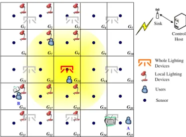
In this paper, we design an intelligent light control system using WSNs with considering user requirements. As shown in Fig. 1.1, we divide the network into grids. In a grid, there is a

Control Host Whole Lighting Devices Users Sensor Local Lighting Devices Sink G1 G2 G3 G4 G5 G6 G7 G8 G9 G10 G11 G12 G13 G14 G15 G16 G17 G18 G21 G22 G23 G20 G19 G25 G24 A B

Figure 1.1: The network scenario of our system.

fixed sensor nodes deployed at the center. These sensors form a multi-hop ad hoc network. One node serves as the sink of the network, and it is connected to the control host. The control host can issue light control commands and config the network. In our system, lighting devices are divided into whole lighting devices and local lighting devices. A whole lighting device is the light such as fluorescent light, which can provide illuminations for several grids. For example, in Fig. 1.1, the light locates in the middle of the network can illuminate grids G7, G8, G9, G12,

G13, G14, G17, G18, and G19. On the other hand, a local lighting device is the one such as table

lamp, which can only provide concentrated illumination. Each user brings a wireless sensor, which is used to locate user’s location and sense the light intensity of the surface that user needs local illuminations.

We assume that users have different requirements based on their activities. For example, in Fig. 1.1, user A is watching television and user B is reading. User A may only specify whole lighting devices to provide sufficient illuminations. But, user B specifies both whole lighting devices and a local lighting device to provide sufficient illuminations at the same time. In this paper, the control host adaptively decides the illumination goals of lighting devices according to users’ requirements. In this paper, we discuss two kinds of illumination requirements: one is fixed user requirement and the other is personalized user requirement. When using the fixed user requirements, two users are considered to have the same illumination requirement if their activities are the same. One the other hand, when using the personalized user requirement, users can specify their illumination requirements according to their activities. We will separately discuss the formulations and solutions for these two requirements. And then device control algorithms adjust the dimmers of lighting devices to achieve the illumination goals. Unlike [21] and [24], our system does not need to know all possible combinations of dimmer levels and

locations to light intensities.

The rest of this paper is organized as follows. Section 2 presents the system architecture. Section 3 and Section 4 introduce the illumination decision algorithms for fixed user require-ment and personalized user requirerequire-ment, respectively. Section 5 presents the device control algorithm for lighting devices. Section 6 shows our prototyping results and Section 7 concludes this paper.

Chapter 2

System Architecture

2.1 System Model

In the following, we define the relationships between grids, users, and lighting devices. Assume

that, in this system, there are k grids, n users, m whole lighting devices, and m0 _{local lighting}

devices. We label those k grids as G1, G2, ..., and Gk. In each grid, a fixed sensor is used

to measure the light intensity of that grid. Fixed sensors periodically report the sensed light intensity to the sink. The control host saves those reported readings by a k × 1 column vector

Sf = h sf_(G 1) sf(G2) · · · sf(Gk) i_T , where sf_(G

i), ∀i ∈ [1, k], means the sensory reading of the fixed sensor sfi in grid Gi. In this

system, we consider that lighting devices have limited capability. For a whole lighting device

wdj, we define the maximum light intensity wdj can provide as lmax(wdj). The control host

records this information by an m × 1 column vector

Lmax wd = h lmax_(wd 1) lmax(wd2) · · · lmax(wdm) i_T .

For a local lighting device ldj, we define the maximum light intensity ldj can provide as

lmax_(ld

j). The control host records this information by an m0× 1 column vector

Lmax

ld =

h

lmax_{(ld1) l}max_{(ld2) · · · l}max_(ld

m0) i_T

.

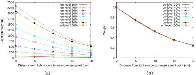
Then we define the relationship between the lighting devices and grids. Like radio signals, light signals degrade with distance. Here, we do a simple experiment to characterize this phe-nomenon by measuring the light intensity of a table lamp at different distances. Fig. 2.1(a) shows the measured intensity of the lamp turned on at different levels. The intensity at 0 cm is considered as the light intensity directly supplied by the lamp. We observe that the measured

0 250 500 750 1000 1250 1500 1750 2000 2250 2500 0 5 10 15 20

Light intensity (lux)

Distance from light source to measurement point (cm) on-level 30% on-level 40% on-level 50% on-level 60% on-level 70% on-level 80% on-level 90% on-level 100% 0 0.2 0.4 0.6 0.8 1 0 5 10 15 20 Weight

Distance from light source to measurement point (cm) on-level 30% on-level 40% on-level 50% on-level 60% on-level 70% on-level 80% on-level 90% on-level 100% (a) (b)

Figure 2.1: An experiment for characterizing the light degradation.

light intensity degraded following a trend, which can be obtained by normalizing the measured light intensity to the one at 0 cm. Fig. 2.1(b) shows the result. From the above observation, we

define a weight w_ij as the measured light intensity of a fixed sensor sf_i contributed by device

wdj is the current light intensity supplied by device wdj multiplies by wij. The control host

maintains the weights by a k × m matrix

W =       w1 1 w12 · · · w1m w1 2 w22 · · · wim ... ... ··· ... w1 k wk2 · · · wkm      .

We assume that weight values can be obtained at deployment stage. The complexity for mea-suring the weight will be O(km). On the other hand, we assume that a local lighting device can only have effect on the illumination of a grid and the illumination provided by local light devices will not affect the measured light intensity of fixed sensors.

By the definition of W , we discuss how to obtain the current light intensity provided by

wdj, denoted as lc(wdj). We first define an m × 1 column vector Lcwdas

Lc_wd = h lc_(wd 1) lc(wd2) · · · lc(wdm) i_T .

Physically, we can say that each whole lighting device wdj is belonged to one grid loc(wdj).

Here, we construct an m × m matrix ˆW by selecting the loc(wdj)-th row, ∀j ∈ [1, m], from W .

From [24], we can know light intensities are additive. The light intensity provided by lighting devices is obtained by subtracting the light intensity provided by the sunlight from the measured

intensity provided by all whole lighting devices can be obtained by ˆ

Sf _{= ˆW · L}c

wd⇒ Lcwd = ˆW−1· ˆSf (2.1)

On the other hand, the light intensity provided by a local lighting device ldj, denoted as lc(ldj),

can be simply obtained by subtracting the light intensity provided by the sunlight and whole lighting devices from the measured light intensity. The control host records the lighting intensity

provided by local lighting devices by an m0_{× 1 column vector}

Lc_ld = h lc_(ld 1) lc(ld2) · · · lc(ldm0) i_T .

In this system, each user brings a portable wireless sensor. The control host judges which grids that users locate by the signals emitted from portable wireless sensor. For example, in

Fig. 1.1, user A and B are located in G25and G16, respectively. A portable wireless sensor is

used to sense the light intensity of the surrounding area (or working area) of a user. Portable sensors also report measured readings to the control host through wireless links. And the control host can record this information by an n × 1 column vector

Sp ₌h_sp_(u

1) sp(u2) · · · sp(un) i_T

,

where sp_(u

i), ∀i ∈ [1, n], means the sensory reading of the portable sensor spi of user ui. We

assume that a local lighting device can only serve one user at a time. We define an m0_{×n matrix}

C to record the corresponding user of a local lighting device.

C =       c1 1 c12 · · · c1n c2 1 c22 · · · c2n ... ... ··· ... cm0 1 cm 0 2 · · · cm 0 n      ,

where cj_i, ∀j ∈ [1, m0_{] and ∀i ∈ [1, n], is 1 if the user i is the corresponding user of the device}

j. Otherwise, cj_i is 0.

This system controls the lights according to users’ activities. Different activities will have different user requirements. At a time instance, each user can have a user requirement. Users can specify their current activities by wireless sensors. In this paper, we further consider two kinds of user requirements settings.

1. Fixed user requirement: In this setting, the system decides user requirements of differ-ent activities for users. A user requiremdiffer-ent is divided into two parts. The first part is the illumination demand of whole and local lighting and the second part is the needed

illumination ranges of whole lighting. The illumination demand of a user ui is defined as:

0 0.1 0.2 0.3 0.4 0.5 0.6 0.7 0.8 0.9 1 0 100 200 300 400 500 600 700 800 245 555 Satisfaction value

Sensory reading (Lux)

Threshold Preference interval

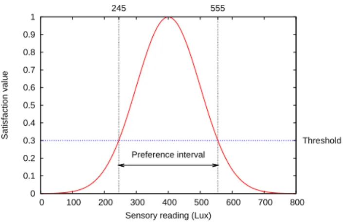
Figure 2.2: A preference function of a user with mean is 400 and variance is 100.

• Demand on whole lighting: [Dl

wd(i), Duwd(i)], where Dlwd(i) and Duwd(i) are the lower bound and upper bound of the demand on whole lighting, respectively.

• Demand on local lighting: [Dl

ld(i), Duld(i)], where Dlld(i) and Duld(i) are the lower bound and upper bound of the demand on local lighting, respectively.

The system also decides illumination ranges for users. The control host records which

grids are required to provide sufficient illuminations for a user ui by a k × 1 column

vector Ri = h ri(G1) ri(G2) · · · ri(Gk) i_T ,

, where, ∀j ∈ [1, k], ri(Gj) = 1 if Gj is located in the illumination range of user ui.

Otherwise, ri(Gj) = 0.

2. Personalized user requirement: In this setting, users decide their requirements. A user requirement is divided into two parts. The first part is the illumination satisfaction of whole and local lighting and the second part is the needed illumination ranges of whole lighting. The definition of illumination satisfaction is similar with the utility function in

[24]. For each activity, a user uispecifies two mean values, µwi and µli, as whole and local

lighting demands, respectively, and two variance values, σw

i and σil, as whole and local

lighting demands, respectively. We define the illumination satisfaction of a user uiby two

functions

• Satisfaction of whole lighting: pw

i (x) = exp(

−(x−µw

i)2

2(σw

i )2 ), where x is the measured

light intensity.

• Satisfaction of local lighting: pl

i(x) = exp(

−(x−µl i)2

2(σl

i)2 ), where x is the measured light

The output values of these two functions will be between 0 and 1, where 0 and 1 mean that the user is the least and most satisfied, respectively. Fig. 2.2 illustrates an example. From Fig. 2.2, we can see that this user most likes the light intensity of 400 lux. When the light intensity degrades or upgrades, the satisfaction of this user will decrease. For the second part, each user can specify which grids the whole lighting devices need to provide

illumination. For each user ui, ∀i ∈ [1, n], the control host maintains a Ri to capture the

user ui’s illumination range requirement.

2.2 System Flows

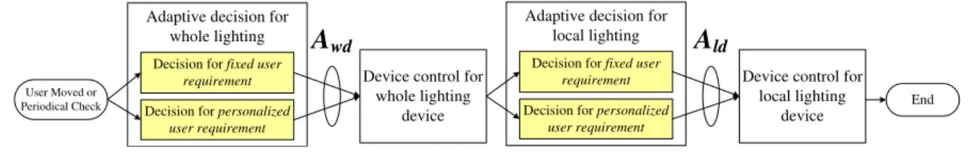
Fig. 2.3 shows the system flow of our light control system. System operations are triggered by a user’s movement or by changes of the environment. Our system first adaptively decides the illumination of whole lighting devices.

• When using the fixed user requirement, our system tries to find the illumination which

can minimize the power consumption under the constraint that users’ requirements can be satisfied.

• When using the personalized user requirement, we aim to provide illumination to

maxi-mize the summation of all users’ satisfaction values under the constraint that each user’s satisfaction is larger than a threshold ¯t. For example, when setting ¯t = 0.3 and a user’s preference as Fig. 2.2, we should provide illumination in the interval (denoted as

prefer-ence interval) [245, 555] for the user.

The outcomes of the whole lighting decision will be an m × 1 column vector

Awd = h

a(wd1) a(wd2) · · · a(wdm)

i_T

,

where a(wdj), ∀j ∈ [1, m], is the needed adjustment for whole lighting device wdj. For

ex-ample, if lc_(wd

j) = 300 lux and a(wdj) = 50 lux, we need to level up wdj to provide a light

intensity of 350 lux. After deciding the illumination, our system adjusts devices by a device control algorithm. The control algorithm utilizes fixed sensors’ feedbacks to adaptively adjust light settings. The goal is to quick converge to the desired illumination.

After adjusting whole lighting devices, local lighting devices compensate illuminations to satisfy users’ requirements on local lighting. Our system makes decisions of local illumination that can minimize the power consumption or maximize users satisfactions when using fixed or personalized user requirements, respectively. The control host decides the adjustments for each

User Moved or

Periodical Check End

Device control for whole lighting

device Decision for personalized

user requirement

Decision for fixed user

requirement

Adaptive decision for local lighting

Decision for personalized

user requirement

Decision for fixed user

requirement

Adaptive decision for whole lighting

Device control for local lighting

device

A

A

Figure 2.3: The system flow of our light control system.

local lighting device. The outcomes will be an m0_{× 1 column vector}

Ald = h

a(ld1) a(ld2) · · · a(ldm0) i_T

,

where a(ldj), ∀j ∈ [1, m0], is the needed adjustment for local lighting device ldj. Then the

device control algorithm controls local lighting devices by utilizing the feedbacks from portable sensors.

Chapter 3

Adaptive Decisions for Fixed User

Requirement

3.1 Decision for Whole Lighting Devices

We model the adaptive decision for fixed user requirement as a linear programming formula. Before presenting the formulation, we first introduce two needed notations. The first one is

matrix ¯Ri, ∀i ∈ [1, n] constructed from Ri, ∀i ∈ [1, n]. An ¯Ri is constructed by the following

rules. For the l-th element ri(Gl) in Ri, generate an element ¯ri(Gl) with the same value with

ri(Gl) at position (l, l). For all other elements in ¯Ri, assign to 0.

¯ Ri =       ri(G1) 0 · · · 0 0 ri(G2) · · · 0 0 ... · · · ... 0 0 · · · ri(Gk)      .

We can notice that an ¯Riis a k × k matrix. The second one is a 1 × m row vector, where each

element in Xmis 1. Xm = h 1 1 · · · 1 i .

The Xmmatrix is used to sum all variables in our formulations.

In the proposed linear programming formula, the objective is to minimize the power con-sumption of whole lighting devices while satisfy users’ requirements. The formula is defined as follows.

Objective:

Preprocessing step Original

formulation

Solve the formula using the Simplex

Algorithm feasible Loosen users' illumination demands End Yes No

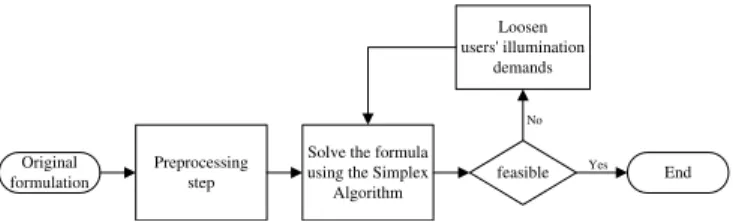
Figure 3.1: The flow of the adaptive decision for fixed user requirement. Subject to:

Dl

wd(i)Ri ≤ ¯Ri(Sf + W Awd) ≤ Dwdu (i)Ri, ∀i ∈ [1, n] (3.2a)

O ≤ Awd+ Lcwd ≤ Lmaxwd (3.2b)

In Eq. (3.1), Awd + Lcwd means the set of light intensities provided by all whole lighting

devices. The object is to minimize the light intensities provided by whole lighting devices to

conserve power. Eq. (3.2a) is the constraint for satisfying user requirements. Sf _{+ W A}

wd represents light intensities of grids after light adjustment. The Eq. (3.2a) means that the light

intensities of the grids located in the illumination range of a user ui should be bounded by

[Dl

wd(i), Duwd(i)]. Eq. (3.2b) is to confine the adjusted light intensity of a device because that

the maximum capability of a whole lighting device wdj is lmax(wdj).

In general, the above formulation can be solved using the Simplex algorithm [6]. But, in some cases, the above formulation may be infeasible, i.e. there is no solution. For example, assume that there are two users located in one grid. If one user is reading and the other is sleeping, their demands will be contradicted. If possible, our system should satisfy all users’ demands. Otherwise, most users’ demands should be satisfied. However, reference [22] shows that find a feasible subsystem of a linear system by eliminating the fewest constraints is NP-hard. In this paper, a preprocessing step is used to check if there exists constraints, which make the formula infeasible. If so, these constraints will be eliminated. Then the control host executes the Simplex algorithm to solve the formulation. If the Simplex algorithm can not find a solution, which means that the formulation is still infeasible after the preprocessing step. In this case, the control host carefully loosens users’ illumination demands until the solution can be found. The decision flow is shown in Fig. 3.1.

The purpose of preprocessing step is to eliminate constraints which cause the formula in-feasible. We propose two checking methods.

• Illumination demand interval check: For each grid Gi, find the users ¯U, whose

illumina-tion ranges contain Gi. Check if the illumination demands of ¯U are intersected. If not,

greedily eliminate Gi from the illumination range of a user in ¯U until the illumination

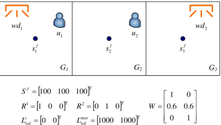
G1 G2 G3 f s_{1 s}f 2 f s₃ 1 wd wd₂ 2 u 1 u > @T R1 1 0 0 » » » ¼ º « « « ¬ ª 1 0 6 . 0 6 . 0 0 1 W > @T R2 0 1 0 > @T f S 100 100 100 > @T c wd L 0 0 max > @T wd L 1000 1000

Figure 3.2: An example of adaptive decision for whole lighting devices.

• Possible illumination check: By the definition of Sf_{, L}c

wd, and Lmaxwd , we can compute the

minimum and maximum possible illumination of grids as Sf_{−W L}c

wdand Sf+W (Lmaxwd −

Lc

wd). For each grid Gi, find the users ¯U, whose illumination ranges covered Gi. For each

user u in ¯U, check if u’s illumination demand intersects with the minimum and maximum

possible illumination of Gi. If not, eliminate Gifrom the illumination range of user u.

After the preprocessing step, the formulation may be still infeasible. When the Simplex

algorithm can not find a solution, the constraints of users will be loosened. For each user ui,

∀i ∈ [1, n], ui’s illumination demand will be changed to [Dwdl (i) − α, Duwd(i) + α], where α is a constant.

3.1.1 Example

We present an example to demonstrate the proposed formulation. In the Fig. 3.2, there are

3 grids, 2 users and 2 whole lighting devices. Assume that user u1’s illumination demand of

whole lighting is [200, 400] and the demand of user u2is [300, 500]. And other used parameters

are listed in Fig. 3.2. Objective: min h 1 1 ià "_a(wd 1) a(wd2) # + " 0 0 # !

⇒ min (a(wd1) + a(wd2)) (3.3)

Constraint of u1: 200    1 0 0    ≤    1 0 0 0 0 0 0 0 0          100 100 100    +    1 0 0.6 0.6 0 1    " a(wd1) a(wd2) #    ≤ 400    1 0 0   

⇒    200 0 0    ≤    100 + a(wd1) 0 0    ≤    400 0 0    (3.4) Constraint of u2:    0 300 0    ≤    0 100 + 0.6a(wd1) + 0.6a(wd2) 0    ≤    0 500 0    (3.5) Constraints of devices: " 0 0 # ≤ " a(wd1) a(wd2) # + " 0 0 # ≤ " 1000 1000 # (3.6)

The above can be solved by the Simplex algorithm. The result of a(wd1) and a(wd2) will be

182 and 152, respectively.

3.2 Decision for Local Lighting Devices

In the following, we decide the Ald. From C, we can know the relationships betweens users and

local lighting devices. For each element cj_i = 1 in C, we can obtain the following equation

Dl_ld(i) ≤ a(ldj) + sp(ui) ≤ Duld(i).

Since our goal is to minimize the power consumption, we can adjust local lighting devices to fit

the lower bounds of user requirements. The Aldcan be computed by the following procedures.

For each local lighting device ldj, if there is an element cji = 1, where 1 ≤ i ≤ n, set a(ldj) =

Dl

ld(i) − sp(ui). Otherwise, set a(ldj) = −lc(ldj). Note that if a(ldj) < −lc(ldj), set a(ldj) =

−lc_(ld

j), and, if a(ldj) + lc(ldj) > lmax(ldj), set a(ldj) = lmax(ldj) − lc(ldj).

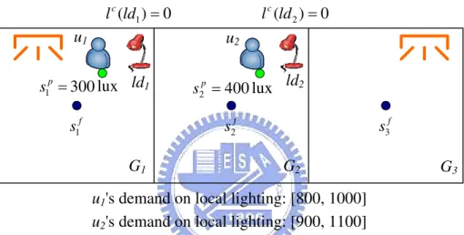
Fig. 3.3 shows an example. Assume that user u1’s illumination demand of local lighting is

[800, 1000] and the device ld1 needs to serve the user. The light intensity measured by sensor

sp₁ = 300 lux and lc_(ld

1) = 0. Thus, the a(ld1) will be 800 − 300 = 500 lux. Similarly, the

G1 G2 G3 f s1 f s2 f s3 300 1 p s ld1 s₂p 400 ld2 u1 u2

u1's demand on local lighting: [800, 1000] u2's demand on local lighting: [900, 1100]

lux lux 0 ) (ld₁ lc lc(ld₂) 0

Figure 3.3: An example of adaptive decision for local lighting devices when using fixed user requirements.

Chapter 4

Adaptive Decisions for Personalized User

Requirement

4.1 Decision for Whole Lighting Devices

We define a non-linear programming formula for personalized user requirement. The goal is to maximize satisfaction of users under the constraint that users’ satisfaction values should be greater than or equal to a satisfaction threshold ¯t. For ease of presentation, in the objective,

we further define a function P0

i : R(k×1) → R(k×1) for an user ui that Pi0(A) = A0, where

A = [axy] ∈ R(k×1) and A0 = [a0xy] ∈ R(k×1) by a0xy = pwi (axy). And, in the constraints,

the preference interval of a user ui is [pil(i), piu(i)], where pil(i) = µi − σi

p

−2 ln(¯t) and

piu_{(i) = µ}

i + σi p

−2 ln(¯t). The formula is listed as below.

Objective: max n X i=1 (Ri)T · Pi0(Sf + W Awd) (4.1) Subject to: pil_(i)R

i ≤ ¯Ri(Sf + W Awd) ≤ piu(i)Ri, ∀i ∈ [1, n] (4.2a)

O ≤ Awd+ Lcwd ≤ Lmaxwd (4.2b)

As shown in (4.1), a user ui’s satisfaction is the summation of the satisfaction values in ui’s

illumination range. The objective is to maximize all users’ satisfactions. Eq. (4.2a) is to restrict the satisfaction value in the illumination ranges of users should be larger than a threshold ¯t. Eq. (4.2b) is to confine the adjusted light intensity of whole lighting devices.

We solve the formulation by a sequential quadratic programming (SQP) [3] method. The basic idea of SQP is as follows. Given a non-linear formula, SQP first reformulates the original

one by a quadratic programming subproblem using a give approximate solution xk_{. Then, SQP}

uses the solution of the subproblem to construct a better approximation xk+1_{. The process is}

iterated to create a sequence of approximations that will converge to an optimal solution x∗_.

As in Section 3.1, in some cases, we cannot satisfy all users. Here, we can apply the pre-processing in Section 3.1 to check if the users’ preference intervals are overlapped. If the formulation is still infeasible, we greedily decrease the threshold ¯t to ¯t− γ, where 0 < γ ≤ ¯t, until there is a solution can be found.

4.1.1 Example

We present an example to demonstrate the proposed formula. The scenario is the same as

Fig. 3.2. We assume that (µw

1, σw1) of user u1is (300, 100) and (µw2, σw2) of user u2is (400, 100).

Besides, we define ¯t = 0.3, which implies the preference intervals of user u1 and u2 are [145,

455] and [245, 555], respectively. Objective: max h 1 0 0 i P∗ 1       100 100 100    +    1 0 0.6 0.6 0 1    " a(wd1) a(wd2) #    + h 0 1 0 i P∗ 2       100 100 100    +    1 0 0.6 0.6 0 1    " a(wd1) a(wd2) #    ⇒ max h 1 0 0 i P∗ 1       100 + a(wd1) 100 + 0.6a(wd1) + 0.6a(wd2) 100 + a(wd2)       + h 0 1 0 i P∗ 2       100 + a(wd1) 100 + 0.6a(wd1) + 0.6a(wd2) 100 + a(wd2)       ⇒ max pw

Constraints of u1: (300 − 100√−2 ln 0.3)    1 0 0    ≤    1 0 0 0 0 0 0 0 0          100 100 100    +    1 0 0.6 0.6 0 1    " a(wd1) a(wd2) #    ≤ (300 + 100√−2 ln 0.3)    1 0 0    ⇒    145 0 0    ≤    100 + wa1 0 0    ≤    455 0 0    (4.4) Constraints of u2:    0 245 0    ≤    0 100 + 0.6a(wd1) + 0.6a(wd2) 0    ≤    0 555 0    (4.5) Constraints of devices: " 0 0 # ≤ " a(wd1) a(wd2) # + " 0 0 # ≤ " 1000 1000 # (4.6)

After applying SQP, we obtain the result of a(wd1) and a(wd1) are 200 and 300,

respec-tively.

4.2 Decision for Local Lighting Devices

In the following, we decide the Ald for personalized user requirements. Similar to Section 3.2,

we first obtain the relationships betweens users and local lighting devices from C. The goal is

to adjust local lighting devices that can maximize the satisfaction of users. The Aldis computed

by the following procedures. For each local lighting device ldj, if there is an element cji = 1,

where 1 ≤ i ≤ n, find a setting of a(ldj) such that pli(a(ldj) + sp(ui)) = 1. Otherwise, set

a(ldj) = −lc(ldj). Note that if a(ldj) < −lc(ldj), set a(ldj) = −lc(ldj), and, if a(ldj) +

lc_(ld

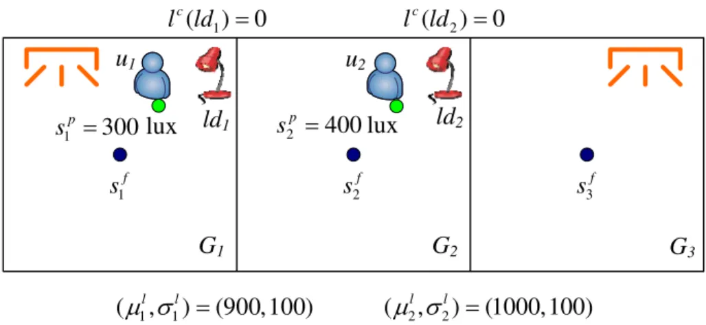
G1 G2 G3 f s₁ s₂f s₃f 300 1 p s ₂p 400 s ld1 ld2 u1 u2 ) 100 , 900 ( ) , (P₁l V₁l ( 2, 2) (1000,100) l l V P lux lux 0 ) (ld₁ lc lc(ld₂) 0

Figure 4.1: An example of adaptive decision for local lighting devices when using personalized user requirements.

Fig. 4.1 shows an example. User u1 specifies (µl

1, σl1) as (900, 100) and the device ld1needs

to serve the user. The illumination measured by the sensor sp₁ = 300 lux and lc_{(ld1) = 0. Thus,}

in order to let pl

1(a(ld1) + 300) = 1, we can set a(ld1) = 600 lux. Similarly, the adjustment

Chapter 5

Device Control Algorithm

The object of this algorithm is to adjust lighting devices to provide sufficient illuminations decided by the above decision algorithms. We use two column vectors

GDwd = [gd(wd1) gd(wd2) · · · gd(wdm)]T and GDld = [gd(ld1) gd(ld2) · · · gd(ldm0)]T to

record the adjustment goals of devices, where GDwd = Awd + Lcwd and GDld = Ald + Lcld,

respectively.

In this paper, we assume that the relationships between the on-levels and the provided light

intensities of devices are unknown. After obtaining GDwdand GDld, this algorithm performs a

closed-loop control mechanism to find on-level settings to achieve GDwd and GDld. The main

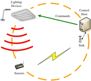
idea of the closed-loop control is to perform a binary search on the on-levels of devices. The procedure is shown in Fig. 5.1. At beginning, the control host decides on-level settings for devices and then sends commands to control dimmers. After adjustment, sensors report light intensities to the control host. The control host can judge if the light intensities provided by

devices achieve GDwd and GDld. If not, the control host decides new on-level settings with

reduced search spaces. Fig. 5.2 shows the control flow. We use the example in Section 3.1.1 to

explain the procedure of our device control algorithm. The a(wd1) = 184 lux and a(wd2) = 150

lux. Assume that wd1 and wd2 are not turned on. The gd(wd1) and gd(wd2) will be 184 lux

and 150 lux, respectively.

• Round 1: We set on-levels of wd1 and wd2 as 50% and 50%, respectively. Assume the

current light intensities provided by wd1 and wd2 are both 500 lux. Since 500 6= 184 and

500 6= 150, the goals are not reached.

• Round 2: Since 500 lux is larger than 184 lux and 150 lux, the on-levels of wd1 and wd2

must be located in level [0, 50%]. The control host will decide level 25% and 25% for wd1

and wd2, respectively. Assume the current light intensities provided by wd1and wd2 are

Commands Control Host Sink Lighting Devices Sensors

Figure 5.1: Mechanism of closed-loop device control.

Start Send command to dimmers Compute the goal of each device Decide devices' on-levels by binary search Wait feedback from sensors Estimate or End Check if achieving wd GD orGD_ld c ld L c wd L

Figure 5.2: Flow of device control algorithm.

• Round 3: Since 270 lux is larger than 184 lux and 150 lux, the on-levels of wd1 and wd2

must be located in level [0, 25%]. The control will decide level 12.5% and 12.5% for wd1

and wd2, respectively. Assume the current light intensities provided by wd1and wd2 are

both 150 lux. Device wd2 achieves gd(wd2). The control process continues in the same

way until wd1 achieves gd(wd1).

Note that when controlling the whole lighting devices, the control host uses feedbacks from

fixed sensors to estimate Lc

wdby Eq. (2.1). On the other hand, when controlling the local lighting

devices, the control host uses feedbacks from portable sensors to estimate Lc

ld. Also note that,

in practice, the on-levels of dimmers are discrete and have finite levels. When control lighting

devices, we can relieve the goals GDwdand GDldto goal intervals. Moreover, during the device

provided by devices and on-levels of devices. The control host can use this information to accelerate the device control procedure.

Chapter 6

Prototyping Results

6.1 Implementation

In this section, we present the implementation of our system in detail. Fig. 6.1 shows the architecture of our intelligent light control system. Wireless sensors collect illuminative values in the room and report to the sink. Then, the control host does a suitable decision by adaptive decision algorithm and triggers actions to adjust the whole and local lighting devices. Fig. 6.2 shows the prototyping result of our system. We built our system in a room with a size of 5 × 5 meters and divided into 3 × 3 grids. To implement the system, we design a protocol stack, as shown in Fig. 6.3. The protocol stack can be divided into three parts: wireless sensor network, actuators, and control host. We briefly describe each part separately in the following section.

6.1.1 Wireless Sensor Network

We use the MICAz mote [7] with light sensor board designed by ourselves as the sensor node, as shown in Fig. 6.4. The MICAz mote is an IEEE 802.15.4 compliant wireless module and operations in 2.4 GHz. We use Si photodiode [23] to design a light sensor due to that the original light sensor with MICAz mote is not accurate enough to support our need.

In our system, two types of messages must be reported to the sink: reporting message and

updating message. The reporting message contains sensory data and the updating message

con-tains users’ activities and location information. In order to support these two types of messages, we form a heterogeneous wireless sensor network which contains two kinds of sensor nodes with different functionalities. The first kind of sensor node is fixed sensor. The fixed sensors sense the illumination in each grid and transmit reporting message to the sink periodically. The second kind of sensor node is portable sensor. The portable sensors are carried by the users and used to identify each user and users’ locations. Also, the portable sensors can measure the

EDX-F04 ADAM-4520 Control host Sink PowerLinc LampLinc RS485 RS232 PowerLine RS232 Local Lighting Devices Whole Lighting Devices UPnP control server Ethernet RS232 DMX

Figure 6.1: System architecture of the intelligent light control system.

Sensors Whole lighting

devices

Local lighting devices

Portable Sensors Fixed Sensors Sensor Handler User Tracking Decision Handler Device Controller Decision Data Administrative User Interface

Control Host

Sensors Report Commands Device Settings Trigger Illumination Location Update WSN Actuators Packet Forwarder Device Control Adaptive Decision Algorithm INSTEON Lighting Devices UPnP

Figure 6.3: Protocol stack of the intelligent light control system.

MICAz Mote Si photodiode Buttons

illumination of work surface for the users and report users’ activities by pressing the button on light sensor board. The portable sensors report reporting message and updating message to the sink node periodically. In order to get users’ location information, we adopt a simple localizing scheme for our system. The portable sensors carried by users overhear the reporting messages of fixed sensors around the users. If the strongest signal beyond a threshold is overheard by portable sensors in a period of time, the portable sensors send an updating message to the sink to announce user’s location information.

The sink, which is connected to the control host via a RS232 interface, collects the reporting and updating messages from each sensor node in the system. The Packet Forward component receives the collected messages from the sink and forwards the messages to the Sensor Handler of the control host.

6.1.2 Actuators

For the actuators, we use two control protocols to control whole and local lighting devices in our current implementation. The whole lighting devices in Fig. 6.5 are controlled by UPnP [29] protocol. We adopt the dimmer and controller manufactured by SmartHome [25] to control the local lighting devices. These two kinds of lighting devices have 101 levels, ranging from 0% to 100% degree of luminance, for adjustment.

UPnP is a set of computer network protocols defined by the UPnP Forum. The UPnP control server sends the UPnP device control message to UPnP-enabled devices through Internet. The UPnP control server uses RS232 to connect ADAM-4250 [1], which is a converter that converts RS232 to RS485. The ADAM-4250 connects to an EDX-F04 [10], which is four channel DMX dimming pack and can adjust four lighting devices. We implement the UPnP Lighting Controls V1.0 standard [29] in our current implementation. When the UPnP control server receives commands from the Device Controller interface of control host, UPnP control server sends on-level commands to adjust the whole lighting devices.

We use the INSTEON LampLinc v2 and PowerLinc controller v2 produced by SmartHome [25] as the dimmer and controller to control local lighting devices, as shown in Fig. 6.6. The dimmer can be controlled by the controller device remotely through the power-line network. Dimmer and controller should be plugged in the outlet and use the protocol designed by the SmartHome to communicate with each other. Dimmer and controller have an unique INSTEON address assigned by the manufacturer to identify the devices. The controller is connected to the control host via an RS232 interface. When the controller receives the command from the Device

Controller interface of control host, controller sends an on-level command to the dimmer to

Figure 6.5: UPnP-enabled whole lighting devices.

INSTEON LampLinc

INSTEON PowerLinc Controller

6.1.3 Control Host

The control host is the core of our lighting system. We implement it in Java programming language. The control host is composed of five components: Sensor Handler, User Tracking,

Decision Handler, Device Controller, and Administrative User Interface. Except the Device

Controller, other components are implemented by Java thread and concurrently handle the tasks.

• Sensor Handler: The Sensor Handler receives the reporting and updating messages from

the Packet Forward component of WSN. Based on the types of messages, Sensor Handler does following actions. If the message is a reporting message, the Sensor Handler has to translate the sensory data to the reading of standard unit. Take light for example, Sensor Handler translates the raw data of illuminative value to lux. Then, the Sensor Handler stores the sensory data into a table such that the data can be queried by other components. If Sensor Handler receives the updating message, it dispatches the message to the User Tracking component.

• User Tracking: The User Tracking component keeps and checks the newest users’

loca-tions and activities. If someone changes his/her location or activity, User Tracking sends triggers to the Decision Handler to adjust the lighting devices to satisfy the users’ needs.

• Decision Handler: Decision Handler is the main component of the control host. It

im-plements the adaptive decision algorithms in Section 3 and Section 4 and device con-trol algorithms in Section 5. When the Decision Handler receives the triggers from the User Tracking component or a periodical checking timer expires, it starts to execute the adaptive decision algorithms. According the sensory data, users’ locations, users’ activ-ities, and users’ requirements, Decision Handler will execute the decision algorithm to compute a proper illuminative value for all lighting devices. We solve the linear or non-linear programming model in adaptive decision algorithms by MATLAB and translate the MATLAB program to Java program by MATLAB Builder for Java [17]. According to the results of decision algorithms, Decision Handler sends device settings to the Device Controller to adjust lighting devices.

• Device Controller: The Device Controller is an interface between the control host and

the actuators. Device Controller sends UPnP commands to UPnP control server through Internet to adjust the whole lighting devices. Also, Device Controller sends INSTEON commands to INSTEION controller through RS232 interface to adjust the local lighting devices.

Monitor panel Configuration panel Information panel

Figure 6.7: Administrative User Interface at control host.

• Administrative User Interface: Fig. 6.7 is an Administrative User Interface, including Monitor Panel, Configuration Panel, and Information Panel. The Monitor Panel

rep-resents that users’ locations and the positions of whole lighting devices. Through the Configuration Panel, administrators can manage the system. Information Panel shows the system information such as light reading, signal strength of sensor nodes, etc. Fig. 6.8 is the dialog for setting system information, such as grid size, the number of devices, and fixed users’ requirement, etc.

Chapter 7

Conclusions and Future Works

In this work, we have presented an intelligent light control system that can automatically control lighting to satisfy each user’s illuminative requirement. Besides, utilize WSNs to collect and re-port illumination of environment and user’s information. The user requirement is decided by the current activity of the user. Fixed user requirement scheme can satisfy each user’s illuminative demands which are set by our system according to users’ current activities for background light and concentrated light. On the other hand, personalized user requirement scheme obtains users’ requirements for different activities from users and attempts to maximize total satisfaction of each user to guarantee that satisfaction of each user should be above a predefined threshold. If the indoor environment has adequate sunlight, we can use the external light to reduce the energy consumption of lighting devices and still satisfy each user’s requirement. The device control algorithm forms a closed-loop to control lighting to achieve the optimal illumination which is computed by decision algorithm for each device. We implement our the system in an indoor environment. While our system detects that users move or change activity in the space, our system adjusts the lighting to satisfy users’ requirements.

We only discuss how to control lighting in an indoor environment. We can not directly apply our system to other environmental factors, such as sound, temperature, and humidity. In our future work, we can improve our system to adapt other environmental factors. Besides, the users’ preference must be beforehand in our system. Hence, in the future, we can design a learning system to obtain the users’ preference automatically such that our system would be more suitable to real life

Bibliography

[1] Adam-4250. http://www.advantech.tw/products/Model Detail.asp.

[2] J. Bachrach, R. Nagpal, M. Salib, and H. Shrobe. Experimental results and theoreti-cal analysis of a self-organizing global coordinate system for ad hoc sensor networks.

Telecommunications Systems Journal, 26(2-4):213–234, 2004.

[3] P. T. Boggs and J. W. Tolle. Sequential quadratic programming. Acta Numerica, 4:1–51, 1995.

[4] D. Braginsky and D. Estrin. Rumor routing algorithm for sensor networks. In Proc. of

ACM Int’l Workshop on Wireless Sensor Networks and Applications (WSNA), 2002.

[5] S. Capkun, M. Hamdi, and J.-P. Hubaux. GPS-free positioning in mobile ad-hoc networks. In Proc. of Hawaii Int’l Conference on Systems Science (HICSS), 2001.

[6] T. H. Cormen, C. E. Leiserson, R. L. Rivest, and C. Stein. Introduction to Algorithms 2nd

Edition. The MIT Press and McGraw-Hill Book Company, 2001.

[7] Crossbow technology Inc. http://www.xbow.com/.

[8] T. Dam and K. Langendoen. An adaptive energy-efficient MAC protocol for wireless sen-sor networks. In Proc. of ACM Int’l Conference on Embedded Networked Sensen-sor Systems

(SenSys), 2003.

[9] Design and construction of a wildfire instrumentation system using networked sensors. http://firebug.sourceforge.net/.

[10] Edx-f04. http://www.liteputer.com.cn/china/liteputer-tw/product.asp.

[11] Habitat monitoring on great duck island. http://www.greatduckisland.net/technology.php. [12] W. R. Heinzelman, A. Chandrakasan, and H. Balakrishnan. Energy-efficient communica-tion protocols for wireless microsensor networks. In Proc. of Hawaii Int’l Conference on

[13] C.-F. Huang, Y.-C. Tseng, and L.-C. Lo. The coverage problem in three-dimensional wire-less sensor networks. In Proc. of IEEE Global Telecommunications Conference

(Globe-com), 2004.

[14] M. Kochhal, L. Schwiebert, and S. Gupta. Role-based hierarchical self organization for wireless ad hoc sensor networks. In Proc. of ACM Int’l Workshop on Wireless Sensor

Networks and Applications (WSNA), 2003.

[15] Q. Li, M. DeRosa, and D. Rus. Distributed algorithm for guiding navigation across a sensor network. In Proc. of ACM Int’l Symposium on Mobile Ad Hoc Networking and

Computing (MobiHoc), 2003.

[16] C.-Y. Lin and Y.-C. Tseng. Structures for in-network moving object tracking in wireless sensor networks. In Proc. of Broadband Wireless Networking Symposium (BroadNet), 2004.

[17] Matlab Builder for Java. http://www.mathworks.com/products/javabuilder/.

[18] S. Meguerdichian, F. Koushanfar, M. Potkonjak, and M. B. Srivastava. Coverage problems in wireless ad-hoc sensor networks. In Proc. of IEEE INFOCOM, 2001.

[19] D. Niculescu and B. Nath. DV based positioning in ad hoc networks. Telecommunications

Systems Journal, 22(1-4):267–280, 2003.

[20] F. O’Reilly and J. Buckley. Use of wireless sensor networks for fluorescent lighting control with daylight substitution. In Proc. of Workshop on Real-World Wireless Sensor Networks

(REANWSN), 2005.

[21] H. Park, M. B. Srivastava, and J. Burke. Design and implementation of a wireless sensor network for intelligent light control. In Proc. of Int’l Symposium on Information

Process-ing in Sensor Networks (IPSN), 2007.

[22] J. Sankaran. A note on resolving infeasibility in linear programs by constraint relaxation.

Operations Research Letters, 13(1):19–20, 1993.

[23] Si photodiode s1133. http://jp.hamamatsu.com/en/index.html.

[24] V. Singhvi, A. Krause, C. Guestrin, J. H. Garrett, and H. S. Matthews. Intelligent light control using sensor networks. In Proc. of ACM Int’l Conference on Embedded Networked

Sensor Systems (SenSys), 2005.

[26] K. Sohrabi, J. Gao, V. Ailawadhi, and G. J. Pottie. Protocols for self-organization of a wireless sensor network. IEEE Personal Communications, 7(5):16–27, October 2000. [27] Y.-C. Tseng, S.-P. Kuo, H.-W. Lee, and C.-F. Huang. Location tracking in a wireless sensor

network by mobile agents and its data fusion strategies. In Proc. of Int’l Symposium on

Information Processing in Sensor Networks (IPSN), 2003.

[28] Y.-C. Tseng, M.-S. Pan, and Y.-Y. Tsai. Wireless sensor networks for emergency naviga-tion. IEEE Computer, 39(7):55–62, 2006.

[29] Upnp forum. http://www.upnp.org.

[30] Y.-J. Wen, J. Granderson, and A. M. Agogino. Towards embedded wireless-networked in-telligent daylighting systems for commercial buildings. In Proc. of IEEE Int’l Conference

on Sensor Networks, Ubiquitous, and Trustworthy Computing (SUTC), 2006.

[31] W. Ye, J. Heidemann, and D. Estrin. An energy-efficient MAC protocol for wireless sensor networks. In Proc. of IEEE INFOCOM, 2002.