國立交通大學
統計學研究所
博士論文
非線性隨機效應剖面資料之無母數監控方法
Nonparametric Monitoring Schemes for Nonlinear
Profiles with Random Effects
研 究 生:鄭清仁
指導教授:洪志真 博士
非線性隨機效應剖面資料之無母數監控方法
Nonparametric Monitoring Schemes for Nonlinear Profiles with Random
Effects
研 究 生:鄭清仁 Student:Ching-Ren Cheng
指導教授:洪志真 博士 Advisor:Jyh-Jen Horng Shiau
國 立 交 通 大 學
統 計 學 研 究 所
博 士 論 文
A Thesis
Submitted to Department of Statistics
College of Science
National Chiao Tung University
in partial Fulfillment of the Requirements
for the Degree of
Doctor of Philosophy
in
Statistics
September 2012
Hsinchu, Taiwan, Republic of China
非線性隨機效應剖面資料之無母數監控方法
研究生:鄭清仁 指導教授:洪志真博士
國立交通大學統計學研究所
摘 要
隨著現代工業製程的進步,品質的特性經常是以應變量(response)
與共變量(covariate)的函數關係呈現,也就是文獻裡所謂的剖面
資料(profile)
。因此,為了因應實際的需求,發展剖面資料的管制
方法是必要的。近年來亦有多篇文獻探討該議題。此篇論文對於具隨
機效應的剖面資料提供了完整的管制方法。首先,我們先考慮服從常
態分配的剖面資料。為了提升管制方法的效率,我們利用主成分分析
得到其主成分記分(principal component score),並利用該記分來
發展管制圖。在此論文,我們對於常態分配的剖面資料分別探討在第
一階段(Phase I)和第二階段(Phase II)的分析。在實際的應用
裡,資料經常並非服從常態分配的假設。因此,在沒有假設資料分配
的情況下,我們亦發展剖面資料的管制方法。為此,我們先對於多變
量資料,發展無分配假設(distribution-free)的第一階段管制方
法。在第一階段的分析,我們利用型一錯誤(type-I error)及型二
錯誤(type-II error)來當作衡量準則。而在第二階段的分析裡,
我們利用平均運行步長(average run length)來衡量。透過模擬分
析,我們所發展的管制方法對於各種製程的變化都能有效地偵測,包
含平均位置的位移、資料散佈的位移或是函數形狀的改變。我們亦利
用真實的資料來示範我們所提出的方法的適用性及效率。
Nonparametric Monitoring Schemes for Nonlinear
Profiles with Random Effects
Student: Chin-Ren Cheng
Advisor: Dr. Jyh-Jen Horng Shiau
Institute of Statistics
National Chiao Tung University
Hsinchu, Taiwan
Abstract
As modern technology advances in many industrial processes, the quality char-acteristics are often gathered in the form of a relationship between the response variable and explanatory variable(s), which are often referred to as profiles in the literature. Therefore, developing schemes for monitoring various types of func-tional characteristics becomes necessary for practical use and has attracted many researchers in resent years. The purpose of this dissertation is to provide a compre-hensive analysis for profiles with random effects. First, the case of the profiles fol-lowing the Gaussian distribution is considered. To monitor the profiles efficiently, the principal component scores of profiles obtained from the principal component analysis are utilized to construct control charts. Both the Phase I analysis and Phase II monitoring for Gaussian profiles are discussed in this dissertation. Since the Gaussian assumption may be violated in many practical applications, we also develop a distribution-free control chart for profiles. To this end, we first develop a novel distribution-free Phase I control chart for multivariate data. Then, two distribution-free control charts for profile data are constructed for Phase I and
Phase II applications, respectively. The type-I and type-II error rates are consid-ered as the performance measures for Phase I analysis whereas the average run length is used for Phase II analysis. Our simulation studies indicate that the pro-posed control charts are efficient in detecting shifts in various kinds of aspects, including the mean, dispersion, and shape of the profile. Some real data analysis are also provided to demonstrate the applicability and effectiveness of the proposed control charts.
誌 謝
包含在中正大學的日子,我的博士班生涯終於要在第六年結束了。這六年的日子 裡,不論是做研究的精神或是對於統計的知識,都得到了很大的進步。從一開始 考上中正大學的博士班,完成碩士論文推廣的研究,又考過了資格考;接下來推 甄上了交大,又考了一次資格考,接著從洪志真老師的指導之下拿到了博士學 位。這一路雖然辛苦,但是在大家的勉勵及幫助之下也算順利。 首先第一個要感謝的當然是我的指導老師:洪志真老師。如果沒有洪老師每週耐 心地和我討論問題和研究方法,我也不會如此順利的拿到學位。還有我在中正大 學的指導老師:黃郁芬老師。感謝他當初啟發了我對作研究的興趣且一起共同完 成了三篇論文。幸運的是:我的兩位指導老師對於學生都相當的親切也都很關心 學生,也讓我在學習的過程中備感溫馨。感謝當初在中正大學另一位老師:王太 和老師。雖然他現在已經轉往美國任教,我還是十分感謝他對我的幫助,不論是 教學或是研究都令我非常印象深刻。感謝大陸南開大學的鄒長亮老師給予我很多 幫助。另外,當然還要感謝交大和清大所有的老師,還有特地從美國回台授課的 魏武雄老師和黃俊宗老師。感謝口試委員們:曾勝滄老師、黃榮臣老師、鄭少為 老師以及王秀瑛老師。感謝他們對於我的論文提出的建議及改進。 感謝一起在研究室奮鬥的學長姐、同學及學弟妹。也感謝常常一起打球並且在統 研盃奮戰過的所有人,讓我在課業之餘有一個抒發的管道。也感謝在中正的學長 姐們,偶而大家可以一起互相勉勵。還有系辦助理:郭碧芬和劉怡君小姐。在交 大這幾年也多虧了她們幫我們解決了許多行政及電腦的問題。 最後當然要感謝我的家人:老爸、老媽和姐姐們。她們所對我付出的關心和支持 是無可取代的。另外還有我的女朋友玉卿,我這幾年的博士班生涯如果沒有她我 也不知道自己能不能支持下去。也要感謝中正大學讓我們在嘉義相遇並相戀。 接下來當學生的日子結束了,往後的日子挑戰還更大。要能夠在社會上有立足之 地,還需要大家繼續的支持及鼓勵。真誠地感謝。 清仁 2012/09Contents
Contents . . . i
List of Tables . . . iv
List of Figures . . . vii
1 Introduction 1 2 Literature Review and Background 4 2.1 Literature Review . . . 4
2.1.1 Phase II Analysis . . . 4
2.1.2 Phase I Analysis . . . 6
2.1.3 Dimension Reduction Methods . . . 7
2.1.4 Distribution-Free Methods . . . 8
2.1.5 Multivariate Process Monitoring . . . 9
2.2 Background . . . 12
2.2.1 Symmetry Property of a Distribution . . . 12
2.2.2 Concept of Spatial Sign . . . 14
2.2.3 Multivariate Sign Test . . . 15
2.2.4 Multivariate Spatial Median . . . 18
2.2.5 Multivariate Sign-Based Control Chart for Phase II Appli-cation . . . 20
3 Profile Monitoring Schemes under Gaussian Assumption 25 3.1 Phase I Monitoring . . . 26
3.1.1 Model Assumptions and Data Smoothing . . . 26
3.1.2 Phase I Monitoring Scheme . . . 28
3.1.3 Performance Measures . . . 30
3.2 Phase II Monitoring . . . 31
3.2.1 Methodology . . . 31
3.2.2 Control Limit Determination and ARL Calculation . . . 34
3.2.3 Diagnosis . . . 35
3.3 Simulation Studies . . . 36
3.3.1 Model Description . . . 36
3.3.2 Phase I Application . . . 38
3.3.3 Phase II Application . . . 45
3.4 Real Data Application . . . 55
3.5 Conclusions . . . 61
4 A Distribution-Free Multivariate Control Chart for Phase I Ap-plications 64 4.1 Methodology . . . 65
4.1.1 A Multivariate Sign-Based Control Chart . . . 65
4.1.2 Control Limit Determination . . . 66
4.1.3 One-at-a-Time Procedure . . . 67
4.2 A Comparative Simulation Study . . . 68
4.3 A Real Data Application . . . 78
4.4 Conclusions . . . 82
5 Distribution-Free Profile Monitoring Schemes 84 5.1 Phase I Monitoring . . . 84
5.1.1 Methodology . . . 84
5.2 Phase II Monitoring . . . 88
5.2.1 Methodology . . . 88
5.3.1 Phase I Applications . . . 90
5.3.2 Phase II Applications . . . 101
5.4 Real Data Application . . . 105
5.5 Conclusions . . . 112
6 Conclusions and Future Works 115 A Tables 119 A.1 The Proportion of the Total Variation Explained by the CS Chart in Section 4.2 . . . 120
A.2 Tables of Control Limits of the Multivariate Sign Shewhart Chart . 122 A.3 Table of Control Limits of the Multivariate Sign EWMA Chart . . . 125
A.4 The Results of the Type-I and Type-II Error Study of the Wine Data126 A.5 The Proportion of the Total Variation Explained by the SMSS Chart of Simulations in Section 5.3.1 . . . 127
B 129 B.1 ARL Calculation of The Combined EWMA Chart . . . 129
List of Tables
2.1 Research works in profile monitoring . . . 23 2.2 Research works in multivariate process monitoring. . . 24 3.1 The shifts in mean and/or variance-covariance matrix of the OC
models . . . 38 3.2 The type-I and type-II error rates and their standard errors (in
parentheses) of OC Model (a) for α = 0.05 and δ2 = 0. . . 40
3.3 The type-I and type-II error rates and their standard errors (in parentheses) of OC Model (a) for α = 0.05 and δ1 = 0. . . 41
3.4 The type-I and type-II error rates and their standard errors (in parentheses) of OC Model (b) for α = 0.05 and δ2 = 0. . . 42
3.5 The type-I and type-II error rates and their standard errors (in parentheses) of OC Model (b) for α = 0.05 and δ1 = 0. . . 44
3.6 The type-I and type-II error rates and their standard errors (in parentheses) of OC Model (c) for α = 0.05 and δ2 = 0. . . 45
3.7 The type-I and type-II error rates and their standard errors (in parentheses) of OC Model (c) for α = 0.05 and δ1 = 0. . . 46
4.1 The pI and pII and their standard errors (in parentheses) for Model
(a). . . 72 4.2 The pI and pII and their standard errors (in parentheses) for Model
4.3 The pI and pII and their standard errors (in parentheses) for Model
(c). . . 74 4.4 The pI and their standard errors (in parentheses) of the MSS chart
and Hotelling’s T2 control chart when using the OAAT procedure. . 75
4.5 The pII and their standard errors (in parentheses) of the MSS chart
and Hotelling’s T2 control chart when using the OAAT procedure. . 77
4.6 The type-I and type-II error rates from mixing the level 7 and level 6 wines. . . 80 4.7 The type-I and type-II error rates for mixing the level 7 and level 5
wines. . . 81 5.1 The type-I error rates of the SMSS chart by using the conventional
and OAAT detecting procedures. . . 93 5.2 The type-I and type-II error rates and their standard errors (in
parentheses) of OC Model (a) for α = 0.05 . . . . 94 5.3 The type-I and type-II error rates and their standard errors (in
parentheses) of OC Model (b) for α = 0.05 . . . . 95 5.4 The type-I and type-II error rates and their standard errors (in
parentheses) of OC Model (c) for α = 0.05 . . . . 96 5.5 The type-I and type-II error rates and their standard errors (in
parentheses) of OC Model (d) for α = 0.05 . . . . 97 5.6 The type-I and type-II error rates and their standard errors (in
parentheses) of OC Model (e) for α = 0.05 . . . . 98 5.7 The type-I and type-II error rates and their standard errors (in
parentheses) of OC Model (5.11) for α = 0.05 . . . 100 5.8 The ARL and SDRL of the SMSE and MENPC charts for Models (a)
and (b). . . 103 5.9 The ARL and SDRL of the SMSE and MENPC charts for Models (c)
5.10 The ARL and SDRL of the SMSE and MENPC charts for Model (e). . . 105 A.1 The proportion of the total variation explained by the CS chart for
OC Model (a) . . . 120 A.2 The proportion of the total variation explained by the CS chart for
OC Model (b) . . . 121 A.3 The proportion of the total variation explained by the CS chart for
OC Model (c) . . . 121 A.4 The control limits of the MSS chart under various type-I error rate
α and dimension p for subgroup size n = 5 and 10 . . . 122
A.5 The control limits of the MSS chart under various type-I error rate
α and dimension p for subgroup size n = 15 and 20 . . . 123
A.6 The control limits of the MSS chart under various type-I error rate
α and dimension p for subgroup size n = 25 and 30 . . . 124
A.7 The control limits of the multivariate sign EWMA chart for p = 2 . 125 A.8 The type-I and type-II error rates for size 20 . . . 126 A.9 The proportion of the total variation explained by the SMSS chart
for OC Model (a) and (b) . . . 127 A.10 The proportion of the total variation explained by the SMSS chart
for OC Model (c) and (d) . . . 127 A.11 The proportion of the total variation explained by the SMSS chart
List of Figures
2.1 The scatter plots of a random sample from N2(0, I2) and the
corre-sponding spatial sign vectors. . . 14 3.1 (a) 200 generated profiles from the multivariate normal distribution
with mean and variance-covariance matrix expressed as (3.12) and (3.13), respectively, and (b) the corresponding smoothed estimates. 36 3.2 Plots of IC and OC samples from Model (a)(top row), (b)(middle
row) and (c)(bottom row). . . 39 3.3 The effect-visualizing plots of the first three PCs, µ0± 3νr, r = 1, 2, 3. 49
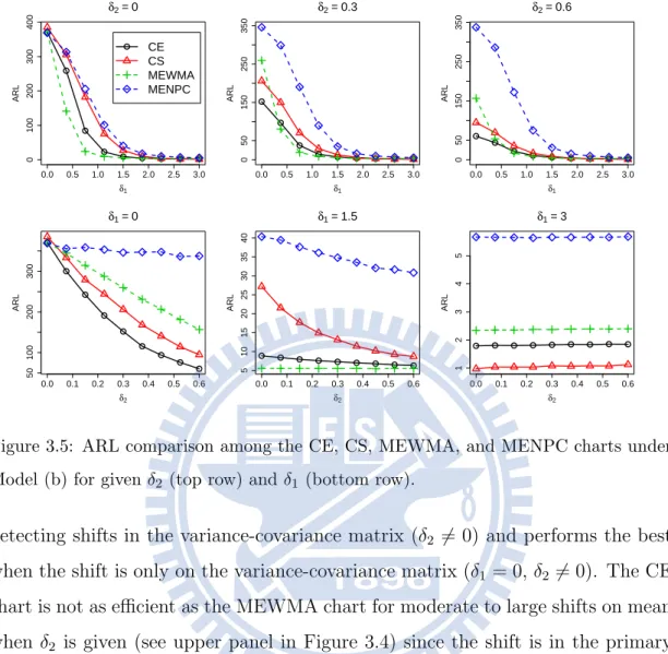
3.4 ARL comparison among the CE, CS, MEWMA, and MENPC charts under Model (a) for given δ2 (top row) and δ1 (bottom row). . . 50
3.5 ARL comparison among the CE, CS, MEWMA, and MENPC charts under Model (b) for given δ2 (top row) and δ1 (bottom row). . . 51
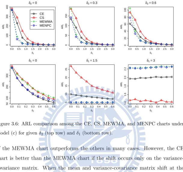
3.6 ARL comparison among the CE, CS, MEWMA, and MENPC charts under Model (c) for given δ2 (top row) and δ1 (bottom row). . . 52
3.7 (a) Plots of the IC and OC profiles from Model (a) before (left panel) and after (right panel) smoothing. . . 53 3.8 (a) The scores of the first three PCs and (b) the scores of the first
three rotated PCs by VARIMAX rotation. . . 54 3.9 The effect-visualizing plots of the first three rotated PCs, µ0 ±
3νr∗, r = 1, 2, 3. . . . 55 3.10 The original and the smoothed profiles of the three of the AEC data. 56
3.11 The first 15 records of the three profiles and their corresponding smoothing estimates. . . 57 3.12 The effect-visualizing plots of the first three PCs, µ0± 3νr, r = 1, 2, 3. 58
3.13 The values of the charting statistics based on T2
0 (panel (a)) and T12
(panel (b)) for the AEC data. . . 59 3.14 The visualized plots of the first three rotated PCs, µ0±3νr∗, r = 1, 2, 3. 60
3.15 The scores of the first three rotated PCs for the AEC data. . . 61 3.16 The 112nd, 115th, 139th, 140th AEC profile and the mean curve. . 62 4.1 (a) - (c) are the scatter plots between variables citric acid (x3),
residual sugar (x4), and density (x8); (d) - (f) are the corresponding
normal Q-Q plots. . . 79 5.1 (a) 200 generated aspartame profiles and (b) the corresponding
smoothing estimates. . . 92 5.2 The scatter plots of the spatial sign vectors of the profiles generated
from OC Models (a) - (e). . . 99 5.3 The plots of the profile segments of variable V3 at step 9. (a) To
show the long-term aging trend from wafer to wafer (the profiles of the last lot are highlighted in red) (b) To show the short-term first-wafer effect within a lot, the first wafer is highlighted in red. . 106 5.4 (a) The plots of the first 222 residual profiles and (b) the
corre-sponding smoothed estimates. . . 108 5.5 (a) The spatial sign vectors of (T2
0, T12)′ and (b) the values of the
charting statistic Q. . . 109 5.6 (a) The first three PCs and (b)-(d) the corresponding effect-visualizing
plots. . . 110 5.7 (a) The plots of the 141 residual profiles used in Phase II analysis
5.8 The values of the charting statistic of the SMSE chart (the dashed line is the control limit of ARL0 = 370). . . 112
5.9 (a) The spatial sign vectors of (T02, T12) (the red circles are the spatial signs detected as OC). (b) The detected OC profiles (red curves) and the reference profiles (black curves). . . 113 5.10 The Q-Q plots of the residual profiles at the first three design points.114
Chapter 1
Introduction
Statistical process control (SPC) has been widely used in various areas, especially in industry. One of the most important purposes in SPC is to monitor crucial quality characteristics of processes/products in order to control the process to stay in a stable state. Among SPC tools, the control chart is a proven effective process monitoring tool used to determine whether the process is in control or not.
The control chart applications are distinguished into Phase I and Phase II with distinct objectives. The objectives of the Phase I application are to bring the process to a state of statistical control and further characterize the in-control process by analyzing historical observations. The control chart would allow the user to collect in-control data by filtering out the abnormal or so-called “out-of-control” (OC) observations in the historical data set. The collected in-control (IC) data are then used to characterize the IC process with a suitable statistical model, which will be used later to construct the control chart in the Phase II application. Since the data used in Phase I analysis are gathered in the past, Phase I analysis is regarded as the retrospective analysis in the literature. Assuming that the process is in statistical control already, the Phase II application emphasizes the online process monitoring of the process characteristics. In this phase, practitioners focus on detecting as efficiently as possible the OC conditions caused by assignable causes
from the future on-going process procedure, Phase II analysis is also regarded as a prospective analysis. Moreover, in Phase II analysis, the necessary process parameters are usually assumed known; that is, they are already known from previous knowledge or are well estimated from the historical data after Phase I analysis.
Traditionally, the quality characteristics that control charts monitor are uni-variate or multiuni-variate random variables. Nevertheless, in many situations, the quality-related characteristic of interest is not a variable or a vector but a func-tional relationship between the response variable and one or more explanatory variables. Under these circumstances, the monitoring focus should be on the func-tional characteristic of the data (referred to as the profile in the literature) instead of on the response values measured at the specific levels of the explanatory vari-ables. In this case, the observations within a profile are often highly correlated and their ordering (as the ordering of the explanatory variables) remains unchanged over time. Moreover, the values of explanatory variables may vary from profile to profile in many situations. Therefore, although profile data look similar to mul-tivariate data, the traditional mulmul-tivariate monitoring schemes often may not be appropriate for profiles. In addition, the profiles observed from a process usu-ally have some features in common and hence exhibit similar patterns. For some cases, the observed profiles can be well represented as a fixed (but needs to be estimated) function plus independent errors, and hence can be suitably modeled by a fixed-effect model. However, for more cases in practice, the profiles in general are of common shapes or similar patterns but still quite different individually, a situation needs to be modeled with a random-effect model or a mixed-effect model to accommodate the profile-to-profile variations. It is noted that, in the literature, the terms “random effects” and “mixed effects” sometimes are used interchange-ably — a random-effect model becomes a mixed-effect model when the mean of the random-effect component is deliberately set to zero by moving the mean into the fixed-effect component.
In this dissertation, we propose some monitoring schemes for profiles with ran-dom effects. We first review related research works in the literature and some background knowledge used in this dissertation in Chapter 2. In Chapter 3, two monitoring schemes for profiles under Gaussian assumption are developed for Phase I and II applications, respectively. In practical use of SPC procedures, the distri-bution of the profiles is often unknown or differs from Gaussian. Before developing monitoring schemes for profile data, we first construct a novel control chart for multivariate observations without distribution assumptions for Phase I applica-tions in Chapter 4. Then, by combining the schemes presented in Chapters 3 and 4, we develop two distribution-free monitoring schemes for profiles in retrospective and prospective analysis, respectively, in Chapter 5. Finally, the conclusion and some directions of future works are given in Chapter 6.
Chapter 2
Literature Review and
Background
This chapter gives a literature review on related research works in process moni-toring and some background knowledge of this dissertation study in Sections 2.1 and 2.2, respectively.
2.1
Literature Review
In this section, we review some previous works in the literature related to our study. For easy reference, we tabulate the reference in profile monitoring and multivariate process monitoring in Tables 2.1 and 2.2, respectively.
2.1.1
Phase II Analysis
The works on the profile monitoring started with the simplest case that the profiles are characterized by a single covariate and the functional relationship can be de-scribed by a linear regression model. Assuming that the intercept and slope in the model are known, Kang and Albin (2000) proposed two approaches to deal with the Phase II profile monitoring problem. One is the Hotelling’s T2 chart based on
the vector of the least squared estimates of the intercept and slope of the incoming profile. The other takes the residuals between the sample profile and the reference profile as a subgroup, then combines the EWMA chart on the average of the resid-uals and the range-chart (R-chart). The authors preferred the second approach. Kim et al. (2003) considered three EWMA control charts for monitoring the esti-mated intercept, slope, and variance of the linear model, respectively. To lessen the correlations among the estimators of the parameters, the centered linear model was considered in their method. Based on the same spirit with the methodology proposed by Kim et al. (2003), Saghaei et al. (2009) utilized the CUSUM chart on the estimated parameters of the simple linear model. Zou et al. (2006) proposed a likelihood ratio (LR) based control chart with a change-point model. To avoid the situation of the paucity of the reference sample, Zou et al. (2007b) developed a self-starting monitoring scheme for linear profiles. In their methodology, the resid-ual and the variance are monitored individresid-ually via two EWMA charts, and the estimated parameters are updated immediately when a new observation arrives. Zhang et al. (2009) constructed a control chart based on the LR to monitor linear profiles. Instead of taking exponentially weighted average of the LR statistic, they sequentially update the estimates of the parameters used in the LR statistic via the EWMA scheme and monitor the corresponding values of the statistic.
In practice, the functional relationship between the response and covariate may not be linear. Kazemzadeh et al. (2009) extended the simple linear model to the polynomial model to fit the profiles. For roundness profile data, Colosimo et al. (2008) considered a spatial autoregressive regression model to account for the continuity in space of the profile, and construct a control chart to monitor the parameters in the model. Vaghefi et al. (2009) developed control charts based on the residuals of the (known) nonlinear model, and several types of metrics were considered to measure the difference between the incoming profile and the reference profile.
covari-ates. Zou et al. (2007a) extended the simple linear model to the general linear model including the polynomial and multiple linear regression models for profile monitoring. Zou et al. (2008) presented a control chart that integrates the usual multivariate EWMA procedure with the generalized likelihood ratio test proposed by Fan et al. (2001).
To be more general, Eyvazian et al. (2011) considered the case of the multiple responses as profiles of multiple covariates, which is the so-called multivariate multiple profiles. They assumed the profiles can be fitted by the multivariate multiple linear regression model and proposed several multivariate control charts to monitor the parameters in the model. Zou et al. (2012a) took the multivariate multiple linear profiles into account and constructed the control chart based on the LASSO-based multivariate control chart proposed by Zou and Qiu (2009). Lee et al. (2011) dealt with the multiple profiles of one covariate in a semiconductor manufacturing process and no linear structure was assumed in their method.
2.1.2
Phase I Analysis
Kang and Albin (2000) suggested that by replacing the EWMA chart to the She-whart chart, their proposed chart can be applied to Phase I analysis. Mahmoud and Woodall (2004) utilized the indicator variables to compare several simple lin-ear regression lines, and considered the F -statistic to identify which of the profiles are out of control. As a generalization of simple linear profiles, Kazemzadeh et al. (2008) discussed that the Phase I monitoring scheme for polynomial profiles. Zhang and Albin (2009) used the χ2 statistic, which is the sum of squared standardized
residuals between the reference profile and the centered profile to be tested, to de-tect the outlying profiles. Similar to the work of Zou et al. (2006), Mahmoud et al. (2007) considered the change-point model in the Phase I monitoring for simple linear profiles.
In the case of the nonlinear model with multiple covariates, Williams et al. (2007a) and Williams et al. (2007b) constructed control charts for the parameters
in the (known) nonlinear model. Jensen et al. (2008) and Jensen and Birch (2009) considered the linear and nonlinear mixed models, respectively, to account for the profile-to-profile variation, and then a T2-type control chart is used to monitor the parameters in the model simultaneously.
For the multiple linear regression profile case, Mahmoud (2008) pointed out that the power of the usual Hotelling’s T2 control chart would be reduced when
the number of the covariates increases. The author regarded the average of the fitted values of the historical profiles as a new covariate; and with that only the simple linear regression model needs to be considered. Since outlying profiles have abnormal values of the parameters in the new model, the parameters were utilized to construct a control chart in Phase I. Parallel to Phase II (Eyvazian et al., 2011), Noorossana et al. (2010) also developed a Phase I monitoring scheme for multivariate multiple linear regression profiles.
2.1.3
Dimension Reduction Methods
In the profile data analysis, profiles are often discretized and hence can be regarded as multivariate data. Since the number of the design points (values of the covari-ate) is usually large, the dimension reduction techniques can be applied to profile data. Jin and Shi (2001) considered the wavelet transformation for the profile and constructed a control chart based on the corresponding coefficients to implement the monitoring scheme. Both the Phase I and II analysis were discussed in their article. Lada et al. (2002) also developed a Phase II control chart based on the wavelet coefficients. For the dimension reduction purpose, a novel minimizing cri-terion was considered to choose a small number of the coefficients. In the use of the wavelet transformation for profiles, Jeong et al. (2006) proposed a T2 chart for
Phase II analysis based on the coefficients for which the deviations from the refer-ence parameters exceed a threshold. Chicken et al. (2009) considered the likelihood ratio statistic of the coefficients to construct a control chart under a change-point
Ding et al. (2006) considered the independent component analysis (ref. Hyv¨arinen et al., 2001) to the wavelet coefficients to reduce the corresponding dimensions in Phase I applications. Shiau et al. (2009) applied the principal component analysis (PCA) to profiles and proposed several control charts based on the scores of the first few effective principal components (PCs) to implement Phase I and II process monitoring.
2.1.4
Distribution-Free Methods
The literature involving distribution-free monitoring procedures for profile data is quite limited. In the development of nonparametric methods, Walker and Wright (2002) pointed out that the smoothing technique is an important tool to summarize and capture the structure of a profile. In addition, the authors used the generalized additive model to fit the profiles and then developed a method to decompose the sources of the variation of profiles; however, no monitoring schemes were provided in this paper. Febrero et al. (2008) considered the depth measure for profiles and detected the outlying cases with lower values of depth. Three types of depthes, including the Fraiman-Muniz depth (Fraiman and Muniz, 2001), h-modal depth (Cuevas et al., 2006), and random projection depth (Cuevas et al., 2007), are con-sidered and the corresponding performances were compared. In Phase II analysis, Cheng (2009) and Wang (2009) respectively considered the simplicial depth (Liu, 1990) and the Oja depth (Zou and Serfling, 2000) to construct the r-chart, Q-chart, and DDMA-chart (Liu, 1995; Liu et al., 2004) by using the PC scores of profiles.
Zou et al. (2009) considered the change-point model integrating with the gen-eralized likelihood ratio (GLR) testing statistic. The GLR statistic measures the difference between the generalized log-likelihood functions under IC (i.e., no change point) and OC (i.e., there exists at least a change point) conditions. Taking each of the profiles as a potential change point, the values of the GLR statistic are cal-culated and then the maximum value is used to determine whether the process is OC or not. Qiu and Zou (2010) constructed a nonparametric profile control chart
by using the smoothed estimates of the scaled residuals of a nonparametric regres-sion model. The authors also presented a self-starting verregres-sion of the monitoring scheme. Qiu et al. (2010) considered the nonlinear mixed effect model to describe profiles to deal with the correlation within a profile, which is a condition usually happen in practice; see Section 3.3.3.
2.1.5
Multivariate Process Monitoring
There are vast amount of papers discussing multivariate process monitoring schemes for either location or dispersion of the process, but only some recent papers are re-viewed here. For more related references, see the papers described in the following and the references cited therein.
Among the multivariate monitoring schemes developed under the multivariate normal distribution, the most popular method could be the Hotelling’s T2 control
chart. It is widely used for monitoring the location of the process in both Phase I and Phase II analysis. However, the Hotelling’s T2 chart is notorious for its poor
power in detecting small location shifts. To get more detecting power for small shifts, Crosier (1988) and Lowry et al. (1992) proposed the multivariate CUSUM and multivariate EWMA control charts, respectively. Mason et al. (2003) pointed out that there would be some special systematic patterns rather than the random pattern in the Hotelling’s T2 chart if some specific conditions occur in the process.
Vargas (2003) and Jensen et al. (2007) proposed their T2 control charts based
on the robust estimators of the location and scatter matrix for Phase I applications. They claimed that the control chart using the minimum volume ellipsoid (MVE) or minimum covariance determinant (MCD) estimator is more powerful in detecting reasonable number of outliers than the regular Hotelling’s T2 control chart. The
use of the scatter matrix estimated by successive difference was also discussed in their papers. Later, Williams et al. (2006) derived the asymptotic distribution of the T2 statistic based on the successive-difference estimator of the scatter matrix.
process mean in both Phase I and Phase II analysis. To avoid a long process of collecting in-control data, Hawkins and Maboudou-Tchao (2007) developed a self-starting EWMA procedure to monitor the process mean. Assuming only a few dimensions of the vector shift, Zou and Qiu (2009) proposed an EWMA control chart integrating the LASSO-based testing statistic.
The aforementioned methodologies focus mainly on monitoring the process mean. Nevertheless, the scatter matrix should also be monitored in real appli-cations. For Phase II applications, Yeh et al. (2004) proposed an EWMA control chart based on the likelihood ratio test statistic for comparing the sample covari-ance matrix of the incoming grouped data with that of the reference sample. Yeh et al. (2005) considered the EWMA of XtXt′, where Xt is the observed vector
at time t, as the estimator of the scatter matrix, and proposed the control charts based on the entries of the estimated scatter matrix to monitor the variability of the process. Huwang et al. (2007) considered not only the EWMA of XtXt′,
but also the EWMA of (Xt− ˆµt)(Xt − ˆµt)′, where ˆµt is the EWMA of Xt, as
the estimators of the scatter matrix. The trace of each estimated scatter matrix was utilized to construct a Shewhart-type control chart. Hawkins and Maboudou-Tchao (2008) adopted the XtXt′ version of the scatter matrix estimator described
above and applied the Alt’s likelihood ratio statistic (Alt, 1984) to monitor the process dispersion. To gain more power than the usual two-sided test on the scatter matrix, Yen and Shiau (2010) derived the likelihood ratio test statistic for testing one-sided alternative hypothesis of increasing process dispersion and developed a control chart accordingly. Yen et al. (2012) further developed an effective chart for detecting dispersion increase and decrease simultaneously by combining two one-sided charts.
Some authors developed multivariate control charts to monitor the location and dispersion of the process simultaneously. Reynolds and Cho (2006) constructed two T2-type control charts based on the EWMA of each component of X
t and
X2
Xt), then combined the two T2 charts to monitor the mean and scatter matrix
simultaneously. Maboudou-Tchao and Hawkins (2011) combined the self-starting monitoring scheme for the mean in Hawkins and Maboudou-Tchao (2007) and the EWMA procedure for the scatter matrix in Hawkins and Maboudou-Tchao (2008) for the same purpose.
The methodologies described above were all developed based on the normality assumption of the observations. However, this assumption is often violated in prac-tice. Stoumbos and Sullivan (2002) and Testik et al. (2003) studied the robustness of the multivariate EWMA control chart. They pointed out that the multivariate EWMA chart is quite robust to normality if one choose a small weighting param-eter λ. But how small λ should be depends on the distribution of the data, which is often difficult to estimate in practical applications. Therefore, distribution-free schemes for process monitoring are definitely in need.
Qiu and Hawkins (2001, 2003) constructed the CUSUM control chart based on the so-called antiranks of vectors, in which the antiranks are the indices of the order statistics. Liu (1995) proposed three control charts, r, Q, and S charts, which can be viewed as the univariate X, ¯X, and CUSUM charts applying on the depth of the
multivariate data. Liu et al. (2004) constructed a nonparametric moving average (MA)-chart derived from the notation of data depth for multivariate data. The simplical depth (Liu, 1990) was considered in their methodology. Hamurkaro˘glu et al. (2004) demonstrated the use of the r and Q charts under the Mahalanobis depth (Mahalanobis, 1936).
Qiu (2008) considered an approach involving the log-linear model to construct a CUSUM chart based on the Pearson’s χ2 statistic. Zou and Tsung (2011)
pro-posed an EWMA monitoring procedure based on the spatial signs of vectors (in-troduced in Section 2.2.5). To incorporate the information in the multivariate data more than just the multivariate direction, Zou et al. (2012b) proposed a spa-tial rank-based multivariate EWMA control chart. In addition, they incorporated the self-starting procedure into the the proposed monitoring scheme. Boone and
Chakraborti (2012) considered the univariate sign and Wilcoxon sign-rank statis-tics for each component of the multivariate data and constructed the Hotelling’s
T2-type control charts based on these distribution-free statistics to monitor the process location.
2.2
Background
Section 2.2.1 reviews several levels of model assumptions often made on distribution symmetry in the literature. Section 2.2.2 introduces the definition of spatial sign and related assumptions. Sections 2.2.3 - 2.2.5 describe some applications of spatial sign, including nonparametric hypothesis testing, robust parameter estimation, and statistical process monitoring.
2.2.1
Symmetry Property of a Distribution
Let y be a p-variate random vector that can be described by the model
y = µ + e, (2.1) where µ is the mean vector and e is the error vector with zero mean and variance-covariance matrix Σ. Assuming that Σ is positive definite, there exists a full-rank
p× p matrix Ω such that Σ = ΩΩ′. Let ε = Ω−1e be the standardized error
vector with zero mean and identity variance-covariance matrix. Then the model (2.1) can be re-written as
y = µ + Ωε. (2.2)
Ω is often called the transformation matrix in the literature. Imposing various
assumptions on the distribution of ε leads to various parametric or semiparametric or nonparametric models. For example, when constructing a semiparametric or nonparametric multivariate test, the symmetry assumption is often needed. The
sense that the distribution is invariant under certain transformations. Note that the assumption made on ε is equivalent to that made on Ω−1(y − µ), hence the connection of the probability density functions (pdfs) between ε and y is that
fy(y) =|Ω|−1fε
(
Ω−1(y − µ)),
where fy and fε denote the pdfs of y and ε, respectively. Oja (2010) provided a
good review about the symmetry property with respect to various kinds of trans-formation. In this dissertation, we only consider the kinds of symmetry described in this section.
Definition 2.1. The random p-vector ε is called elliptically symmetrical (or
spheri-cally symmetrical) if Oε∼ ε, for all orthogonal matrices O. It is called symmetrical
(or centrally symmetrical) if −ε ∼ ε.
Here, the symbol “∼” denotes “is distributed as”. Note that the elliptically symmetrical random vector is also symmetrical since the matrix−Ip is orthogonal.
Thus, the following three “nested” assumptions lead to a hierarchy of symmetrical models:
(A0) ε∼ Np(0, Ip);
(A1) ε is elliptically symmetrical; (A2) ε is symmetrical.
The strongest assumption (A0) is equivalently to the usual assumption, y ∼
Np(µ, Σ), made on random samples in the literature. In many multivariate data
analysis applications, such as principal component analysis (PCA), canonical cor-relation analysis (CCA), and factor analysis (FA), it relies on the assumption (A0) to develop good theoretical properties of the methodologies. Because the assump-tion (A1) or (A2) made on ε is weaker than (A0), it corresponds to a boarder class of distributions. Also, the model based on the assumption (A1) or (A2) may be regarded as a semiparametric generalization of the multivariate normal model
2.2.2
Concept of Spatial Sign
In the univariate case, data can be ordered and the sign of an observation indicates its direction (+1, 0 or −1) from the origin. For any univariate variable y, the following sign function
U (y) = |y|−1y, if y̸= 0, 0, if y = 0,
gives the sign of y. Although there is no such natural ordering for multivariate data, the multivariate sign function can be defined in the same manner as
U (y) = ||y||−1y, if y̸= 0, 0, if y = 0,
for any multivariate vector y, where||·|| is the Euclidean norm. U(y) is called the multivariate (spatial) sign vector of y, and sometimes called the direction vector, since it only indicates the direction of the observation by mapping it on the multi-dimensional unit sphere. For illustration, Figure 2.1(a) and 2.1(b) show the scatter plots of a random sample from the bivariate standard normal distribution and the corresponding spatial sign vectors, respectively.
−4 −2 0 2 4 −4 −2 0 2 4 Original Data x1 x2 (a) −1.0 −0.5 0.0 0.5 1.0 −1.0 −0.5 0.0 0.5 1.0 Spatial Signs x1 x2 (b)
Figure 2.1: The scatter plots of a random sample from N2(0, I2) and the corresponding
Consider again the model assumption issue mentioned earlier in the last section. A broader class of distribution models can be obtained if the assumptions are only made on the sign vector. Let the spatial sign vector of the random vector ε be
u = U (ε). The following assumptions are then considered:
(B1) u is uniformly distributed on the multivariate unit sphere; (B2) u is symmetrical.
The distributions of ε corresponding to the models (B1) and (B2) are named the
elliptical direction distribution and directionally symmetrical distribution,
respec-tively. Note that there is no additional assumption on the distribution of the radius
r =||ε||. The radius r and direction u may be dependent, thus skew distributions
are allowed under models (B1) and (B2). Among the models introduced so far, a hierarchy of the models is straightforward to obtain as follows.
Property 2.1. The models (A0)-(A2) and (B1)-(B2) satisfy the following joint
hierarchy
(A0) ⇒ (A1) ⇒ (A2)
⇓ ⇓
(B1) ⇒ (B2).
The symbol “⇒” denotes “implies”. For the tests or monitoring schemes intro-duced/developed later, we focus on the distribution-free property under the family of elliptical direction distributions. For more details about the spatial sign and symmetrical distribution families, see Chapter 2 of Oja (2010).
2.2.3
Multivariate Sign Test
Consider an independent and identically distributed (i.i.d.) random sample{y1,· · · , yn}
from F (y− θ), where F (·) represents the cumulative distribution function (cdf) of a continuous p-dimensional distribution “located” at θ. Consider testing the null
loss of generality, θ0 is assumed zero; otherwise, simply replace yi by yi− θ0 for
i = 1, . . . , n. In this testing hypothesis problem, different levels of assumptions
were imposed on F in the literature. For example, for yi’s from the multivariate
normal distribution, the well-known Hotelling’s T2 test is a powerful test, which
rejects H0 if
T2 = (n− 1) ¯y′S−1y¯≥ (n− 1)p
n− p Fp,n−p(α),
where ¯y and S are the regular sample mean and sample variance-covariance matrix
of the data, respectively, and Fp,n−p(α) is the upper α quantile of the F distribution
with p and n− p degrees of freedom. However, stronger assumptions made on the cdf F cause more restrictions in using the test. Thus, one would like to construct a powerful test with distribution assumptions to be as weak as possible.
Recall that a test statistic t(·) is said to be affine invariant if t(y1, . . . , yn) =
t(Dy1, . . . , Dyn) for every (y1, . . . , yn) and all nonsingular p× p matrix D. This
property ensures that the test will stay the same under certain transformations of data, e.g., rotating data around the origin or altering the scale of measurements. Note that the Hotelling’s T2 statistic is affine invariant. However, the dependency
on the normality assumption could be a serious drawback for Hotelling’s T2 test and many parametric methodologies. For example, it is hard to control the type-I error probability of the Hotelling’s T2 test at a specified level when the normal assumption is violated. To circumvent this drawback, Randles (2000) proposed a test based on the spatial sign, which provides a robust alternative for testing the hypotheses when the population distribution is unknown.
More specifically, Randles (2000) constructed an affine invariant multivari-ate sign test utilizing the transformation-retransformation approach proposed by Chakraborty et al. (1998) and the directional transformation proposed by Tyler (1987). The transformation-retransformation approach uses a data-determined nonsingular matrix Ay based on y that has an affine-equivariance property; that
then the resulting matrix ADy satisfies
D′A′DyADyD = cA′yAy,
where c is a positive scalar that might depend on D and yi’s. After transforming
the data by Ay, the spatial sign vectors of the transformed data are
ui = U (Ayyi) for i = 1, . . . , n. (2.3)
Following the form of the Hotelling’s T2 test, the test statistic is then constructed
as a quadratic form of the spatial sign vectors,
Q = n ¯u′(AVE{uiu′i} )−1 ¯ u, (2.4) where AVE{Bi} = ∑n
i=1Bi/n denotes the average of Bi’s over i, in which Bi
can be a vector or a matrix; and ¯u = AVE{ui}. For Ay, Randles (2000) adopted
the Tyler’s transformation matrix (Tyler, 1987). Tyler’s method is to find a data-driven scatter matrix, ST, which is a p×p symmetric positive-definite matrix with
trace(ST) = p, such that
AVE{U (ATyi)U (ATyi)′
} = 1
pIp,
for any AT satisfying A′TAT = ST−1. The ST is called the Tyler’s scatter matrix
and AT is the corresponding Tyler’s transformation matrix.
The Tyler’s scatter and transformation matrices are surprisingly easy to com-pute empirically as follows. The iterative procedure begins with S ← Ip as the
initial value, and then transform it to the next value via
S ← pS1/2AVE{uiu′i}S
1/2. (2.5)
Here, “←” means “set to”. Continue updating step given in (2.5) until ||pAVE{uiu′i}−
Ip|| is sufficiently small, where the matrix norm is defined as ||A|| =
√
trace(A′A).
The Tyler’s scatter matrix is then set as ST = [p/trace(S)]S and the corresponding
Tyler (1987) claimed that the Tyler’s scatter matrix ˆST is the “most robust”
es-timator of the scatter matrix for elliptically symmetric distributions, and is unique if the sample is from a continuous p-dimensional distribution with n > p(p− 1). Replacing the Ay in (2.3) by AT, the test statistic (2.4) then becomes
Q = np ¯u′u,¯ (2.6) and H0 is rejected for large values of Q. Randles (2000) showed that the test
statistic Q is affine invariant when n > p(p− 1) and is distribution-free under H0
in the class of elliptical direction distributions. The author also illustrated that the proposed sign-based test is quite powerful under elliptically symmetrical or some skew distributions, and is well competitive to Hotelling’s T2 test and other
nonparametric tests.
2.2.4
Multivariate Spatial Median
The center of the distribution under study is usually unavailable in practice and needs to be estimated from data empirically. Among many statistics, the spatial median is often recommended in the literature for describing the multivariate center due to its robustness.
Definition 2.2. Let {y1, . . . , yn} be a p-variate random sample of size n. The
(sample) spatial median ˆθ is defined as the minimizer of the criterion function
n
∑
i=1
||yi− θ||. (2.7)
Taking the gradient of the objective function (2.7), one sees that if ˆθ solves the
equation n ∑ i=1 yi− ˆθ ||yi− ˆθ|| = n ∑ i=1 U (yi− ˆθ) = 0,
then ˆθ is the desired spatial median. Milasevic and Ducharme (1987) showed that
(2000) provided an algorithm by modifying the Weiszfeld’s algorithm (Weiszfeld, 1937; Weiszfeld and Plastria, 2009) to compute the spatial median. Specifically, the algorithm takes the regular sample median for each dimension as the initial estimate of each component of θ and then iterates the following step
θ ← θ + AVE{U(yi− θ)}
AVE{||yi− θ||−1}
, (2.8)
until convergence. This algorithm is extremely simple and converges quickly and monotonically.
There is a natural link between the spatial median and the Tyler’s scatter matrix as described below. Hettmansperger and Randles (2002) proposed a pro-cedure for estimating the spatial median θ and Tyler’s transformation matrix A simultaneously. The desired parameters (θ, A) satisfy
AVE{U(A(yi− θ))} = 0,
AVE{U(A(yi− θ))U(A(yi− θ))′} =
1
pIp,
and A′A = S−1. These estimators of the location and transformation matrix are called Hettmansperger-Randles (HR) estimators, and are very easy to compute in high dimensions. The iterations are described as follows.
1. Initially set (θ, S) ← ( ˜θ, Ip), where ˜θ is composed of the p regular sample
medians of the p components. Let S1/2 be any p× p matrix such that
S1/2S1/2 = S.
2. Fix S and let zi = S−1/2(yi− θ), for i = 1, . . . , n. Then iterate
θ ← θ + AVE{U(zi)}
AVE{||zi||−1}
until convergence.
3. Fix θ and let zi = S−1/2(yi− θ), for i = 1, . . . , n. Then iterate
until ||pAVE{U(zi)U (zi)′} − Ip|| is sufficiently small, and then let S ←
[p/trace(S)]S.
4. Repeat steps 2 and 3 until both of θ and S converge.
The resulting values of θ and ST are the estimated spatial median and the Tyler’s
scatter matrix. Then the corresponding Tyler’s transformation matrix is an AT
such that A′TAT = ST−1. Unfortunately, there is no proof so far to ensure that
the HR algorithm converges, but it actually works in most of situations. The exis-tence and uniqueness of (θ, A) are shown by Hettmansperger and Randles (2002) for the directionally symmetrical distributions, and hence the elliptical direction distributions. They also showed that the distribution-free property holds for the elliptical direction distributions.
2.2.5
Multivariate Sign-Based Control Chart for Phase II
Application
In Phase II multivariate statistical process control (MSPC), one of the main tasks is to detect the process change as quickly as possible when the process is out of control. Usually, the location parameter is one of the process characteristics of con-cern in practice. Let y−m0+1, . . . , y0 be m0 i.i.d. historical p-variate observations
and yi be the ith future observation collected over time, for i = 1, 2, . . .. Consider
the following multivariate change-point model
yi ∼ F (y− θ0) for i =−m0+ 1, . . . , 0, 1, . . . , τ F (y− θ1) for i = τ + 1, . . . ,
where τ is the unknown change point and θ0 ̸= θ1. Zou and Tsung (2011) proposed
an MSPC methodology incorporating the multivariate sign test (Randles, 2000) and the exponentially weighted moving average (EWMA) scheme for monitoring the location parameter of online sequential observations. Their control scheme is introduced briefly as follows.
Analogous to regular monitoring schemes, the first step is to estimate the loca-tion parameter and transformaloca-tion matrix (or scatter matrix) from the reference sample. For robustness, the HR estimation method introduced in the last section was also recommended in Zou and Tsung’s method. Denote the estimated spatial median and Tyler’s transformation matrix by (θ0, A0). The spatial sign vector of
the observation yi collected online is
ui = U (A0(yi− θ0)) for i = 1, 2, . . . .
Then construct the EWMA sequence by
wi = (1− λ)wi−1+ λui,
where λ is a weighting parameter and u0 = 0. The proposed control chart triggers
a signal if Qi = 2− λ λ pw ′ iwi > L,
where L > 0 is a control limit chosen to achieve a specified in-control (IC) average run length (ARL).
Zou and Tsung (2011) showed that the proposed control chart is affine invari-ant and distribution-free in the sense that the IC ARL is the same for the class of elliptical direction distributions. The distribution-free property not only makes the monitoring scheme robust to the underlying distribution, but also provides a convenient way to determine the control limit L. More specifically, since the IC run-length distribution is the same for any continuous process with an elliptical di-rection distribution, L can be determined from any distribution, e.g., the standard normal distribution. The control limits for some values of p, λ, and IC ARL were tabulated in Zou and Tsung (2011). They claimed that the sign-based EWMA control chart is fast to compute with a computational time similar to the mul-tivariate EWMA (MEWMA, Lowry et al., 1992) and more efficient in detecting
is heavy tailed or skewed. However, when the shift is quite large, the MEWMA chart outperforms the sign-based control chart since the sign-based control chart considers only the directions rather than the distances from the origin.
Table 2.1: Research works in profile monitoring
Distribution Model Phase I Phase II
Kang and Albin (2000) Kang and Albin (2000) Simple Mahmoud and Woodall (2004) Kim et al. (2003) Linear Mahmoud et al. (2007) Zou et al. (2006) Jensen et al. (2008) Saghaei et al. (2009)
Zhang et al. (2009) Williams et al. (2007a) Zou et al. (2007a) Generalized Williams et al. (2007b) Kazemzadeh et al. (2009)
Linear Kazemzadeh et al. (2008) Eyvazian et al. (2011) Mahmoud (2008) Lee et al. (2011)
Gaussian Noorossana et al. (2010) Zou et al. (2012a)
Distribution Nonlinear Jensen and Birch (2009) Colosimo et al. (2008) Vaghefi et al. (2009) Jin and Shi (2001) Jin and Shi (2001)
Lada et al. (2002) Ding et al. (2006) Jeong et al. (2006) Shiau et al. (2009) Nonparametric Zou et al. (2008) (This Dissertation)
Chicken et al. (2009) Shiau et al. (2009) (This Dissertation)
Febrero et al. (2008) Cheng (2009)
(This Dissertation) Wang (2009)
Distribution- Zou et al. (2009)
Free Nonparametric Qiu and Zou (2010)
Qiu et al. (2010) (This Dissertation)
Table 2.2: Research works in multivariate process monitoring
Distribution Detect shift in Phase I Phase II
Vargas (2003) Crosier (1988)
Jensen et al. (2007) Lowry et al. (1992) Mean Zamba and Hawkins (2006) Zamba and Hawkins (2006)
Hawkins and Maboudou-Tchao (2007) Zou and Qiu (2009)
Gaussian Yeh et al. (2004)
Distribution Yeh et al. (2005)
Covariance Huwang et al. (2007)
Matrix Hawkins and Maboudou-Tchao (2008)
Yen and Shiau (2010) Yen et al. (2012)
Mean and Reynolds and Cho (2006)
Covariance Maboudou-Tchao and Hawkins (2011)
Matrix
Liu (1995) Qiu and Hawkins (2001)
Hamurkaro˘glu et al. (2004) Qiu and Hawkins (2003) (This Dissertation) Liu et al. (2004)
Distribution- Mean Qiu (2008)
Free Zou and Tsung (2011)
Zou et al. (2012b) Boone and Chakraborti (2012)
Chapter 3
Profile Monitoring Schemes under
Gaussian Assumption
In this chapter, we consider the problem of profile monitoring when the process is from Gaussian. Equivalently, the discretized profile data are assumed from the model (A0) described in Section 2.2.1. This chapter is organized as follows. Sections 3.1 and 3.2 present the proposed process monitoring schemes for Phase I and II, respectively. Section 3.3 presents results of some simulation studies of our proposed monitoring schemes and performance comparisons between the proposed schemes and some existing methods. Section 3.4 demonstrates the applicability of the proposed control charts with a real example. Section 3.5 concludes this chapter with a brief discussion on some related issues.
3.1
Phase I Monitoring
3.1.1
Model Assumptions and Data Smoothing
Assume the observed profile data can be described by the following nonparametric regression model:
yij = g(xij) + fi(xij) + εij for i = 1, . . . , m, j = 1, . . . , pi, (3.1)
where g(·) is the mean profile function, i.e., the fix-effect term, fi(·) is the
random-effect term of the ith profile, xij is the jth covariate value of the ith profile, and
(εi1, . . . , εipi)′ is the i.i.d. random error vector with mean 0 and variance σε2. The
random-effect term fi and the errors εij are assumed independent of each other. In
this chapter, we assume fi is distributed as Npi(0, Σi), where Σi = [σi,jk]j,k=1,...,pi
and
σi,jk = E[fi(xij)fi(xik)].
The collected profile data are often accompanied with noises. To filter out the noise in the raw data, smoothing profiles as a preprocess step is often adopted. Moreover, the design points of the covariate may vary from profile to profile in real applications, a situation the PCA cannot be applied directly. To cope with this situation, we can simply smooth each individual profile and obtain the values of the smoothed profile at the same set of design points, say, x = (x1, . . . , xp)′ for
a certain p. Many popular smoothing techniques, such as kernel smoothing, local polynomial regression smoothing, smoothing splines, B-splines, and wavelets can be used and they usually make little difference for this purpose.
In this study, the local linear smoothing method (Fan and Gijbels, 1996) is adopted for simplicity. Given any x0 in the range of the design points, the local
linear estimator for the ith profile takes the form of ˜ yi(x0) = p ∑ j=1 Wj(x0)yij for i = 1, 2, . . . , (3.2) Wj(x0) = Uj(x0) /∑p k=1 Uk(x0), Uk(x0) = Kh(xik− x0)[m2(x0)− (xik− x0)m1(x0)], ml(x0) = 1 n p ∑ k=1 (xik− x0)lKh(xik− x0), l = 1, 2,
and Kh(·) = K(·/h)/h with K(·) being a kernel function and h being the
band-width. Generally, the selection of the kernel function K(·) is not crucial (ref. Fan and Gijbels, 1996); thus the popular Epanechnikov kernel,
K(u) = 3
4(1− u
2)I(|u| ≤ 1),
is adopted in this study.
The local linear smoothing technique has been implemented in R, S-plus, and some other statistical softwares and is extensively used in applications. Another benefit of using the local linear smoothing is that the corresponding estimate is a linear combination of the original profile data so that its distribution can be obtained easily from the normality assumption of data. Therefore, we can simply assume the smoothed profiles are distributed as Np(µ, Σ), where µ and Σ are the
mean and variance-covariance matrix of the smoothed profiles, respectively. In the use of the PCA technique, the choice of the number of effective PCs is affected by the degree of smoothness; thus the popular generalized cross-validation (GCV) method proposed by Craven and Wahba (1979) is considered in choosing the smoothing parameter, i.e., the bandwidth in our case. Without repeating smoothing, the GCV method is computationally more efficient than the ordinary cross validation (OCV) method. Moreover, it has been found that the GCV method has a tendency of less under-smoothing than the OCV method. Specifically, for a
given profile y, define the GCV function as GCV(h) = py ′[I p− Wh]y [tr(Ip− Wh)]2 ,
where Ip is the p× p identity matrix and Wh is the smoothing matrix
correspond-ing to a certain bandwidth h. Then the desired bandwidth h is the minimizer of the GCV function. The minimization of GCV(h) with respect to h will inevitably involve trying a large number of values of h. Ramsay and Silverman (2005) in-troduced a greatly-speeding-up computation method by performing a preliminary generalized eigen-analysis. For more details about GCV, see Gu (2002) or Ramsay and Silverman (2005).
3.1.2
Phase I Monitoring Scheme
Let y be a profile datum following model (3.1) and ˜y be the corresponding local
linear smoothing estimate. To simplify notation, we suppress the “∼” symbol and denote the y as a profile datum after smoothing hereafter. During Phase I, the process may not be stable yet and all the parameters necessary for monitoring must be estimated from the data on hand. In this study, we simply use the sample mean vector and sample variance-covariance matrix, denoted as ( ˆµ, ˆΣ), to estimate
(µ, Σ).
The methodologies we propose in this dissertation involves the PCA technique. In functional PCA, the eigen-functions ν(·) and the corresponding eigen-values λ are defined to satisfy the equation
∫
Q(t, s)ν(s)ds = λν(t),
where Q(t, s) is the covariance function; see Ramsay and Silverman (2005). By applying the smoothing technique to profiles as a preprocessing step, we obtain smoothed profiles at a pre-determined set of design points. Thus, the regular PCA can be applied to the smoothed profiles directly. We adopt the notation of the regular PCA in what follows for simplicity. Both of the functional form and
regular form of PCA can be utilized for our purpose, but the function form is more involved in theory and in computation.
In Phase I monitoring, Shiau et al. (2009) proposed a method based on PCA and the Hotelling T2 statistic. The method applies the eigen-analysis to ˆΣ to obtain
the corresponding eigenvalue-vector pairs, denoted as (λ1, ν1), . . . , (λp, νp), where
λ1 ≥ λ2 ≥ . . . ≥ λp ≥ 0. The selection of the “effective” principal components
(PCs) is based on the total variation explained by the chosen PCs along with the principle of parsimoniousness that we often use in variable selection. Let the number of the effective PCs be K. Consider the statistic
T0i2 = (s0i− ¯s0)′B0−1(s0i− ¯s0), (3.3)
i = 1, ..., m, where s0i is the vector of the first K PC scores for the ith profile,
¯
s0 =
∑m
i=1s0i/m, and B0 =
∑m
i=1(s0i− ¯s0)(s0i− ¯s0)′/(m− 1). A large value of
the T2
0 statistic indicates that the corresponding profile could be abnormal and
perhaps should be deleted from the historical data set. Since the score vectors are distributed as multivariate normal asymptotically (Anderson, 2003), according to Tracy et al. (1992) and also Sullivan and Woodall (1996),
m (m− 1)2T 2 0i ∼ Beta ( K 2 m− K − 1 2 ) approximately.
Thus, for a control chart with a false-alarm rate α, the control limit can be set at the upper α quantile of the beta distribution multiply by (m− 1)2/m, and
observations with T2
0i values exceeding the control limit are regarded as OC.
The methodology proposed by Shiau et al. (2009) has a drawback that the information on the PC νK+1, . . . , νp are ignored and thus the changes in the space
spanned by these PCs will not be monitored. To overcome this drawback, we consider another T2 statistic based on the remaining p− K PCs defined as
T1i2 = (s1i− ¯s1)′B1−1(s1i− ¯s1) for i = 1, ...m, (3.4)