Monitoring and Assessment of Control Performance for Single Loop Systems

Industrial & Engineering Chemistry Research is published by the American Chemical Society. 1155 Sixteenth Street N.W., Washington, DC 20036

Article

Monitoring and Assessment of Control Performance for Single Loop Systems

Hsiao-Ping Huang, and Jyh-Cheng Jeng

Ind. Eng. Chem. Res., 2002, 41 (5), 1297-1309 • DOI: 10.1021/ie0101285 Downloaded from http://pubs.acs.org on November 18, 2008

More About This Article

Additional resources and features associated with this article are available within the HTML version: • Supporting Information

• Links to the 2 articles that cite this article, as of the time of this article download • Access to high resolution figures

• Links to articles and content related to this article

Monitoring and Assessment of Control Performance for Single Loop

Systems

Hsiao-Ping Huang* and Jyh-Cheng Jeng

Department of Chemical Engineering National Taiwan University Taipei 10617, Taiwan, Republic of China

The single loop control system with controller of general structure or with PI/PID structure is studied. The control task of the system is to track step set-point changes or reject the intermittent step output disturbances. Performance of a simple feedback system is assessed with its IAE value (J) and its rise time (tr) observed from the response of the system to a step set-point change. Assume that the dynamics of open loop processes can be represented by models of first order or second order plus dead time (i.e., FOPDT or SOPDT). On the basis of these models, the optimal IAEs and the associated rise times are computed. The performance of a system is assessed by comparing its current IAE to the optimal IAEs. An index is thus defined for this quantitative assessment. To be free of a process model for assessment, envelopes of optimal IAE and the rise time are prepared. A method to estimate the step response for set-point tracking by making use of the response of the system to dither inputs is presented. By introduction of dither inputs intermittently to the system, the performance of the single loop can be monitored on-line.

1. Introduction

Assessment and monitoring of control systems have been an active area of research for the past decade.1-7 Many works considered the minimum variance at the output as the control objective, and performance of the system is assessed by computing the ratio of this minimum variance to that of the actual ouput. However, to design for minimum variance control (MVC), ap-propriate models to characterize the inputs such as set-point and the disturbance are required.8_{Unfortunately,} detailed models of both process and disturbance are rarely available, and thus the resulting MVC systems may be extremely sensitive to model mismatch. For this reason and due to some other practical issues, control-lers in chemical plants are almost never implemented with MVC objectives. In stead, they are implemented to minimize some integral indices (e.g., IAE, ISE, etc.) or to achieve some dynamic properties in time domain or frequency domain (e.g., rise time, overshoot, settling time, or bandwidth, etc.). A paper from Åstro¨m9_studied the dynamic properties just mentioned for simple feed-back systems. Although the paper developed techniques for qualitative and quantitative methods for assessing the performance, the methods presented achievable performance with order-of-magnitude estimates. Fur-thermore, the controller considered is designed by the Ziegler-Nichols method. In addition to that, some aspects of monitoring the performance of control loop were also addressed by Eriksson and Isaksson.10_{In their} paper, alternative indices are suggested to cope with the possible difficulty encountered when deterministic in-put, such as step, changes. Lately, Swanda and Seborg11 used settling time in a step response to set-point changes for assessment. Other evaluations on dynamic performances have also been reported in the litera-ture.12-18 _{However, as far as the methods have been} reported, the common deficiency is the lack of address on the limiting performance in terms of penalty on

errors (such as IAE, ISE, etc.) that is achievable within the framework of simple feedback loop, where control-lers of conventional form are used. Without knowing the limiting achievable performance, there would be no indication of the potential improvement that can be obtained from redesigning the controller. Neither would one have indications of the present status of the system or the need for modifications to an advanced control structure.

It is our purpose to consider the assessment of control systems that have conventional controllers instead of the MVC. By the term conventional controllers, it is meant that the controllers are in the form of rational functions of Laplace transformed variable, s, and is physically realizable. As has been mentioned in the paper of Eriksson and Isaksson,10_{it is difficult to assess} the performance of a control loop without specifying the control task. There may be different criteria to define the task for control application. One of the common process control applications is to design a system for tracking step set-point changes and rejecting intermit-tent step output disturbances. In this paper, the single loop system for this objective is considered. The reason for considering this control task is that the system thus obtained has satisfactory performances in both set-point tracking and disturbance rejections without excessive oscillations, although not being optimal for load inputs. The system has acceptable gain and phase margins. A simple feedback system for this control objective may consist of a general controller or of a PI/PID controller. The open-loop process in this simple loop is assumed to be representable with models of simple dynamics such as first order or second order plus dead time (i.e., FOPDT or SOPDT). Achievable optimal IAE (i.e., J*) and the corresponding rise time (t_r/) resulting from the tracking response are thus studied. The optimal per-formances of the simple feedback systems are repre-sented with trajectories of J* and t_r/. The performances of systems that consists of controllers with general or with PI/PID structure are thus assessed. By making use of the trajectories of J* and t_r/, on-line monitoring of * Author to whom all correspondence should be addressed.

E-mail: [email protected]. Fax: 886-2-2362-3935.

10.1021/ie0101285 CCC: $22.00 © 2002 American Chemical Society Published on Web 02/08/2002

the performance of a simple feedback system is thus illustrated.

2. Limiting Achievable Minimal IAE- with General Controllers

Assessment for control systems has been focused on regulation problems subjected to stochastic inputs. A minimum output variance is considered as the limiting performance. The theoretical minimum variance of a control system can be estimated by prewhiting the actual output of the system with the knowledge of the dead time of the open loop process.19 _{Under this} framework of formulation, MVC becomes a benchmark for performance assessment.

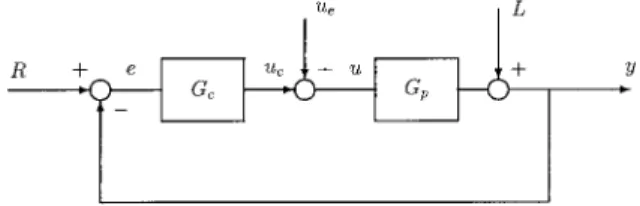
However, as the minimum variance controller is not implemented in most process control applications, the limiting performance based on minimum variance is really not achievable for most control systems, especially for those restricted to PID controllers. Consider a simple feedback system as shown in Figure 1. A controller with a general structure is considered to be in the form of

where the orders of m and n are not constrained except

m e n. As mentioned, the control task considered here

is to track step set-point changes or to reject step output disturbances. In the following, the optimal design by making use of Gc of eq 1 will be studied first. The optimal design is aimed to minimize an IAE perfor-mance index, i.e.

Since the controller is not constrained with its m and

n, the minimal value of J (designated as J*) will be

taken as the performance limit that a simple feedback system can achieve. Then, by considering Gcof PI/PID structure, the actual achievable J_pid/ and J_pi/ will be investigated.

2.1. Limiting Optimal Simple Loop System.

Con-sider the conventional feedback loop as shown in Figure 1. The open loop process Gp(s) and the controller Gc(s) have the general forms of the following equation:

Let Gc(s) be the controller of the simple feedback control system. The product of Gcand Gpis known as the loop transfer function (abbr. LTF) of the system20 and is designated as GLP(s), that is

Then the system error related to the inputs as the following

where, v(s) is considered as a generalized input that enters the system at the same point as that of the set-point, that is

As the input v is taken as a step input which takes into account the drift nature of set-point or disturbance changes, GLPwill be of type I.21Thus, the controller Gc(s) has one integration mode as shown in eq 1.

For single loop systems where IMC controllers are used,22_G

LP(s) can always be given as

where H(s) is a proper and rational function of s with

H(0) ) 1.

To find the optimal value of J, the following minimi-zation problem is considered:

This is subject to

The above performance index J depends on the choice of H(s). Thus, to find the optimal performance, J is minimized by searching for an optimal GLP(s).

Thus, by solving the minimization problem in eq 10, J* together with G_LP/ can be obtained.

To solve the problem presented above in a more general way, let S ) θs, and GLPbecomes

where kho) khoθ and

Minimization of J in eq 10 is equivalent to minimize the integration of |e(S)| subject to eqs 11 and 12. The result minimum IAE is designated as Jh* which is related to J* as

The minimization can be performed by searching for GLP of eq 11. When it is found, substitution of S with θs will give the optimal G_LP/ in terms of s.

Figure 1. Simple feedback control system.

G_c(s) )kc(ams m_{+ a} m-1s m-1_{+ ... + a} 1s + 1) s(bns n_{+ b} n-1s n-1_{+ ... + b} 1s + 1) (1) J )

∫

∏

∏

∫

∫

The GLPhas different functional forms that depend on the designs of the controller in the loop. In general, the GLP should have more poles than zeros. However, since low pass filters with very small time constants can be used to guarantee realizability of the controllers, we shall consider that GLPmay have equal numbers of poles and zeros. We shall call the numbers of such poles as the orders of GLP.

Thus, in searching for the best achievable GLP, we shall focus on the exploring H(s) by sequentially in-creasing its order. The simplest form for GLPis of first order, i.e.

According to eq 12, an optimization procedure is pro-ceeded to find GLPthat minimizes the IAE for tracking the step input of v(s). The result using the Simplex method is found as follows:

Or, it is

The resulting minimum J* is 1.377θ.

Similarly, we proceed to find the best GLPof second order, and the result is

for which J* ) 1.314θ.

Then, for third order, we have

and J* ) 1.310θ.

Notice that the last two results of J* are very close, and the difference is considered insignificant. This shows that a further increase in the order of GLPover four will not give a significant reduction of the minimum IAE value. Thus, the minimum IAE value of the simple feedback system is taken as 1.31θ, and the correspond-ing LTF is the one in eq 18.

It is found that the system that comprises of G_LP/ given above has a gain margin equaling 2 and a phase margin equaling 60 °C. In other words, this system will have reasonable stability robustness. The general con-troller to synthesize the G_LP/ is in the form of eq 1. It is given as

where G_p- is the invertible part of Gp(s), and F(s) is composed of low pass filters with arbitrarily small time constants to make Gc(s) physically realizable.

2.2. Achievable Suboptimal Simple Loop. In

general, chemical processes have dynamics that can be represented by the reduced forms of eq 3 as follows.

•FOPDT (first-order-plus-dead-time) processes:

•SOPDT (second-order-plus-dead-time) processes:

Consider the processes given above: the resulting optimal loop transfer function will not be practically achievable with practical controllers for two reasons. One is that the controller with high order derivatives is not practically implementable. The other is that the controller needs to meet realizability conditions.

If the time unit is properly taken so that the apparent value of θ is small, the best achievable GLP

/

can be approximated to a lower order form of the following equation:

Regarding this GˆLP, the parameters are searched again in order to have suboptimal IAE values. The suboptimal IAE values are found to be 1.38θ, which is the same as the result is eq 15.

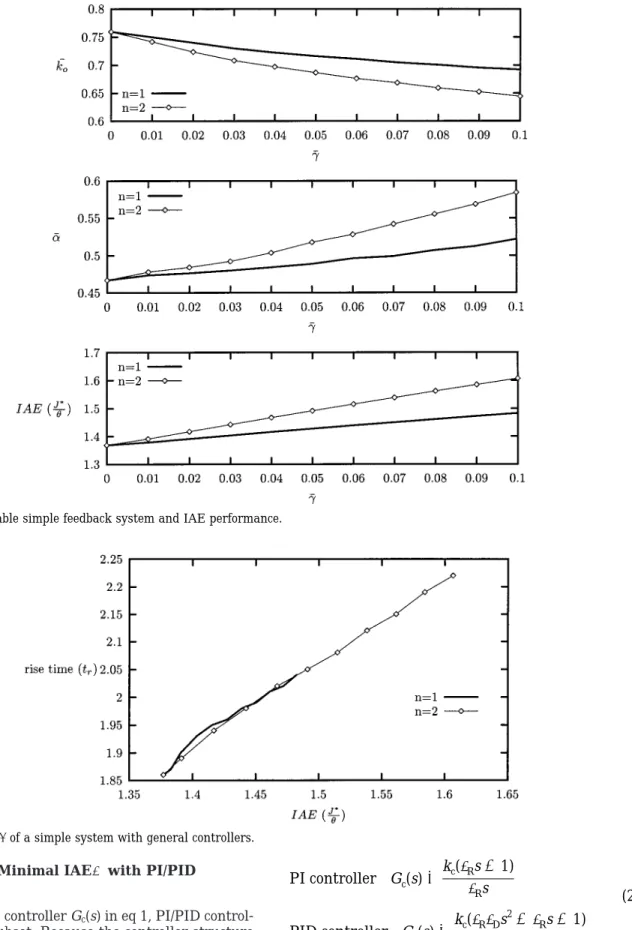
To cope with the realizability issue of Gc(s), the actual achievable GˆLPmay have more filters than the one given above, that is

where 0 e n e 2. The suboptimal results for this practically achievable GˆLPas well as their parameters are thus given in Figure 2. Since the value of γj can be arbitrary small, it is thus found that the best achievable minimum IAE approaches 1.38θ, and the corresponding suboptimal loop transfer function is

2.3. Achievable Minimal IAE with General Con-trollers. The general controller to synthesize G_LP/ has been given in the form of eq 1. It has been shown that the practically achievable J* is 1.38θ. However, taking into account the effect of the filters, the practical value of the minimal IAE will be greater than that of J*. The achievable value of J* (i.e., Jˆ *) depends on the order and the time constants of the filters. They are given in Figure 2 for n ) 1 and 2.

The other important performance that can be ob-tained from the time domain response is the rise time. Since only the type I system is considered, the rise time is taken as the time the system takes to first reach the set-point. This rise time is an indication of the speed of response of the system. The rise times of the suboptimal simple feedback systems are plotted against Jh* in Figure 3. GLP(S) ) kh_o(1 + RjS)e-S S (14) G_LP/ (S) )0.76(1 + 0.47S) S e -S ₍₁₅₎ GLP / (s) )0.76(1 + 0.47θs) θs e -θs (16) G_LP/ (s) )0.83(0.18θ 2 s2+ 0.70θs + 1)e-θs θs (0.30θs + 1) (17) GLP / (s) )0.84(0.25θ 3 s3+ 0.97θ2s2+ 1.71θs + 1)e-θs θs (0.41θ2s2+ 1.26θs+1) (18) G_c(s) ) G_LP/ (s)G_p-(s)F(s) (19) Gp(s) ) k_pe-θs τs + 1 (20) G_p(s) ) kpe -θs τ2s2+ 2τζs + 1 (21) Gˆ_LP≈k h_{o(1 + Rj θs)e}-θs θs(1 + γj θs) (22) Gˆ_LP≈k h o(1 + Rjθs)e -θs θs(1 + γjθs)n (23) Gˆ_LP/ (S) )0.76(1 + 0.47S) S e -S (24)

3. Achievable Minimal IAE- with PI/PID Controllers

Regarding the controller Gc(s) in eq 1, PI/PID control-lers became a subset. Because the controller structure is confined, the best achievable system given above no longer applies. As has been mentioned earlier, the performance of PI/PID control is closely related to the types of models that represent the dynamics of the process. In the following, we shall study the PI/PID control for the two types of simple processes mentioned. The PI/PID controller used is given in the following equations:

3.1. Optimal PI/PID Control Loops. Unlike the

loop transfer function for simple feedback system with general controllers, the loop transfer functions for PI/ PID control loops are closely related to the dynamics of the open loop processes. To find the optimal simple PI/ PID loops, the loop transfer functions as well as the

Figure 2. Achievable simple feedback system and IAE performance.

Figure 3. t_r/vs J*/θ of a simple system with general controllers.

PI controller Gc(s) ) kc(τRs + 1) τRs PID controller Gc(s) ) k_c(τ_RτDs 2_{+ τ} Rs + 1) τRs(τfs + 1) (25)

resulting minimal values of IAE for each of the two types of processes aforementioned are studied. Here, the filter constant τf in PID controller is assumed to be arbitrarily small and can be neglected. As a result, the loop transfer function of a simple PI/PID feedback loop for the FOPDT process will be written as

where kho) kckpθ/τR, Ah ) τRτD/θ2, Bh ) τR/θ, and τj ) τ/θ. Similarly, we can write the loop transfer function of the PID loop for the SOPDT process as follows:

Then, the value of Jh that is subject to a step change of v is minimized by adjusting the parameters kho, Ah , and Bh . The optimal values of IAE (designated as J_pi/ or J_pid/ ) for PI and PID control loops are thus computed, and those data are fitted as shown in Tables 1 and 2.

3.2. Achievable Minimal IAE and Rise Time. The

dynamic performances of the achievable systems are important to the assessment of a current control system in operation. As the results from the previous section, these performances depend on the open-loop processes being controlled. In Tables 1 and 2, the optimal IAE values are given as Jh_pi/ and Jh_pid/ . These values have to be multiplied by θ to become their actual values. That is

For FOPDT processes with PI control, the value J_pi/ is a function of the ratio of τ to θ. Notice that the value of J_pi/ remains approximately constant at 2.1θ when

τj > 5. On the other hand, for τj e 5, 1.7θ e Jpi /

e 2.1θ. For those cases where J_pi/ ≈ 2.1θ, the reset time is approximately equal to the process time constant. This fact has also been observed from many well-known tuning rules.23 _{In case of FOPDT processes with PID}

control, a first-order filter is needed to fulfill the realizability requirement. As a result, the achievable

J_pid/ is a function not only of the ratio of τ to θ but also of the time constant of the low pass filter. If this time constant is taken very small, the achievable IAE will approach to a value of 1.38θ. For both PI and PID control, the rise time of the step response to the set-point is plotted and as shown in Figure 4.

Similarly, for SOPDT processes with PI/PID control, the results of optimal IAE are functions of parameters of open-loop processes. Notice that for PI control loop,

Jh_pi/ is divided into two types by ζ. The first type applies to ζ e 2.0 where Jhpi

/

is a function of τj and ζ. The second type applies to ζ > 2.0 where Jhpi

/

is only a function of the ratio of minor time constant to dead time, τj2. The results for PID control loop are similar to PI one except these two types being divided at ζ ) 1.1. These func-tional forms of Jh_pi/ and Jh_pid/ are given in Tables 1 and 2. PI loop G_LP(s) )kckp(τRs + 1)e -θs τRs(τs + 1) ) kh_o(Bh S + 1)e-S S (τjS + 1) PID loop G_LP(s) )kckp(τRτDs 2_{+ τ} Rs + 1)e -θs τRs(τs + 1) ) kh_o(Ah S2+ Bh S + 1)e-S S (τjS + 1) (26) PI loop GLP(s) ) k_ck_p(τ_Rs + 1)e-θs τRs(τ 2 s2+ 2τζs + 1) ) kho(Bh S + 1)e -S S (τj2S2+ 2τjζS + 1) PID loop G_LP(s) )kckp(τRτDs 2_{+ τ} Rs + 1)e -θs τRs(τ 2 s2+ 2τζs + 1) ) kh_o(Ah S2+ Bh S + 1)e-S S (τj2S2+ 2τjζS + 1) (27) J_pi/ ) Jh_pi/θ J_pid/ ) Jh_pid/ θ (28)

Table 1. Optimal PI Control Loop and Jh_pi/

process Gp(S) GLP(S) ) Gc(S)Gp(S) FOPDT τj e 5 kpe -S τjS + 1 kh_o(Bh S + 1) τjS + 1 e-S S Jh_pi/ ) 2.1038 - 0.6023e-1.0695τj FOPDT τj > 5 kpe -S τjS + 1 0.59e-S S Jh pi / ) 2.1038 SOPDT ζ e 2.0 kpe -S τj2S2+ 2τjζS + 1 kh_o(Bh S + 1) (τj2S2+ 2τjζS + 1) e-S S Jh pi / ) R(ζ)τj2_{+ β(ζ)τj + γ(ζ)} R(ζ) ) 0.7444ζ3_{- 1.4975ζ}2_{+ 1.0202ζ - 0.2525} for ζ e 0.7 R(ζ) ) 0.0064ζ - 0.0203 for 0.7 < ζ e 2.0 β(ζ) ) 1.1193ζ-0.9339for ζ e 2.0 γ(ζ) ) -18.4675ζ2_{+ 17.9592ζ - 2.7222 for ζ e 0.5} γ(ζ) ) -0.0995ζ2_{+ 0.4893ζ + 1.4712} for 0.5 < ζ e 2.0 SOPDT ζ > 2.0 kpe -S (τj₁S + 1)(τj₂S + 1); τj1g τj2 kh o(Bh S + 1) (τj₁S + 1)(τj₂S + 1) e-S S Jh_pi/ ) -0.0173τj22_{+ 1.7749τj2+ 2.3514}

Table 2. Optimal PID Control Loop and Jh

pid / process Gp(S) GLP(S) ) Gc(S)Gp(S) FOPDT τj e 3 kpe -S τjS + 1 k h o(Ah S 2_{+ Bh S + 1)} τjS + 1 e-S S Jh pid / ) 1.38 - 0.1134e-1.5541τj FOPDT τj > 3 kpe -S τjS + 1 0.76(0.47S + 1) e-S S Jh_pid/ ) 1.38 SOPDT ζ e 1.1 kpe -S τj2S2+ 2τjζS + 1 k h o(Ah S 2_{+ Bh S + 1)} (τj2S2+ 2τjζS + 1) e-S S Jh pid / ) 2.1038 - λ(ζ)e-µ(ζ)τj λ(ζ) ) 0.4480ζ2_{- 1.0095ζ + 1.2904} µ(ζ) ) 6.1998e-3.8888ζ+ 0.6708 SOPDT ζ > 1.1 kpe -S (τj₁S + 1)(τj₂S + 1); τj1g τj2 k h o(Bh S + 1) τj₂S + 1 e-S S Jh_pid/ ) 2.1038 - 0.6728e-1.2024τj2

Also, the rise times of these optimal systems are plotted in Figure 5. In fact, to justify which type of controllers fit better to control a given process, the system dynamics is not the only concern. However, from dynamic point of view, one can compare the actual achievable mini-mum IAE resulting from two designs based on different dynamic models. Although both FOPDT and SOPDT models can be used to model the same open-loop dynamics, the apparent dead time of the former is usually larger than that of the latter. Thus, by applying the formula in Tables 1 and 2, two achievable minimal IAE values can be obtained and compared.

4. Assessment of Performance

The assessment of performance should depend on what basis the system is compared with. Since the system with general controller structure has more freedom in re-allocating the dynamic poles, the optimal IAE is more stringent than those with PI/PID control-lers. In the following, the assessment based on these two classes of controller structures will be addressed.

4.1. Assessment of General Controllers. As has

been presented above, if the controller in the loop is not restricted to the PI/PID, the achievable J* is found to be 1.38θ. A similar index to the one used for assessing the MVC system can be defined for assessment:

If the value of J in a current system deviates from the limiting J*, the value of Φ will be less than 1. And, the smaller Φ is, the worse the system performs dynami-cally.

This index Φ defined above can be useful in justifying if a simple feedback structure is adequate for a given process. The portion of the original IAE (i.e., J) that can be reduced by renewing the controller is a major concern. This portion in terms of the fraction of the original IAE is 1 - Φ. On the other hand, if control configuration is not confined to be a simple feedback loop, the optimal performance of the IAE value will be the process dead time (i.e., θ).24_{Thus, the best return}

from renewing the control configuration will be 0.38θ. In other words, in terms of fraction of the original IAE, it is 0.38θ/J.

Using this index Φ, the optimal PI/PID control system can also be assessed and will be discussed in the following section.

4.2. Assessment of PI/PID Controllers. PI/PID

control systems have been widely used in industrial process control. As has been mentioned, the perfor-mances of these PI/PID control systems are very much dependent on the dynamics of the open-loop processes. To understand how well a PI/PID control can perform by referring to the optimal system with general control-lers, efficiency factors for the optimal PI/PID control systems (designated as η*) for FOPDT and SOPDT processes are computed according to the following equation:

It is found that for open-loop processes that have dynamics of second order plus dead time, the efficiency of the PID control is mostly around 65% only. But for FOPDT process, the efficiency is very close to 100%. Thus, compared with the optimal simple feedback system, the PID controller is not so efficient for SOPDT processes.

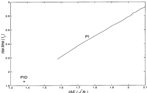
On the other hand, the PID controller has the best efficiency to control the FOPDT processes. The curves of Jh_pi/ and Jh_pid/ vs t_r/as shown in Figures 6 and 7 clearly feature the performance of PI/PID loops. The status of the performance of a PI/PID control loop can be under-stood by locating the point of (Jh, tr) on that figure. If it is far off the optimal region, the system is more away from performing well. Besides, the location of the point indicates the weakness of the system. For example, if the point falls beneath the optimal region, it means the tracking error is resulting from the response being too fast. It seems that the assessment requires the knowl-edge of open-loop dynamics. However, from Figures 6 and 7, it can be seen that the optimal regions form pretty narrow bands. As a result, the performance would

Figure 4. Optimal rise time tr /

of PI/PID control system of FOPDT process.

Φ ) J*

∫

not so sensitive to the parameters. As long as the point (Jh, tr) is located on the bands of the corresponding

controller type, the performance of the system is close to the optimal.

Figure 5. Optimal rise time t_r/of PI/PID control system for SOPDT process: (a) Gp, ζ e 2.0; Gc, PI; (b) Gp, ζ > 2.0; Gc, PI; (c) Gp, ζ e 1.1;

5. Monitoring of Performance

As has been mentioned earlier, the dynamic behaviors are observed from a step response of the system to the input v. Having the IAE value and rise time from this step response the performance of the system can be assessed as presented previously. The most direct way to generate a response is to introduce a step change at the input entrance of v(s). This can be usually done by introducing a step change to the set-point. However, a step change to the set-point will force the system to drift away from it normal operating point. An alternative way to avoid this drift away is to introduce a sequence of stationary dither inputs at the entrance of ueas shown in Figure 1, that is

where ucdesignates the output from the controller, and ue designates the external input introduced. From Figure 1, it is found that the output of the controller,

uc, is given as

which has almost the same functional form as the output y that track the step set-point change except the sign.

Thus, if the dither inputs are introduced at the process input, the negative controller output, -uc, will be taken as the output signal for analysis. For conven-ience, we shall use w(t) to designate the signal -uc. To assess the dynamic performance, the step response to the input v will be reconstructed from this dither output signals. By choosing the frequency of change of dither inputs, a discrete-time model of the following can be identified:

Notice that the apparent dead time, D, of open loop process is a priori knowledge required for this perfor-mance monitoring. It can be estimated using the method of sampled data25 _{or using an open loop step test.}26 These data of the tests are usually available during the stage of controller tuning. In fact, from Figure 1, during the on-line monitoring with dither inputs, the apparent dead time of Gpcan also be estimated from the cross-correlation between the signals y and u. Let

and

Then we have

Thus, with a rectangular data window of length N, the parameter vector P can be estimated as

This modeling problem can be solved with least-squares algorithms (e.g., Ljung27_{). For on-line} monitor-ing, a rectangular data window of proper length during the period when dither inputs are introduced can be used. The step response of the system to a step set-point change can be computed from the resulting model of eq 32. For example, for k ) l ) 2, the estimated step response, wˆ (k), is obtained by solving the following difference equation

with

Figure 6. Trajectory of t_r/vs J*/θ for optimal PI/PID control system of FOPDT process.

W(t) ) [w(t 1) w(t 2) ... -w(t - l)v(t - D)v(t - D - 1) ... v(t - D - k)]T P ) [a₁a₂... a_lb₀b₁b₂... b_k]T wˆ (t) ) W(t)TP (33) P ) Arg min {P} {

∑

Figure 7. Trajectory of t_r/vs J*/θ for optimal PI/PID control system of SOPDT process: (a) Gp, ζ e 2.0; Gc, PI; (b) Gp, ζ > 2.0; Gc, PI; (c) Gp, ζ e 1.1; Gc, PID; (d) Gp, ζ > 1.1; Gc, PID.

Thus, for each data window during which dither inputs are introduced, a step response can be generated. With this generated step response, both values of J and tr can be computed.

Usually, the open loop model of Gpis not identified during the performance monitoring; the targeting point in the trajectory of J* and t_r/is unknown. However, the optimal regions of these trajectories will be helpful. As shown in Figure 8, the envelopes for these trajectories of PI/PID control are plotted, and the equations for these envelopes are given as follows.

•FOPDT Process:

•SOPDT Process:

If a given system has its operational Jh and trlocated inside the envelope, the performance of the system is pretty close to the optimal one. Thus, by locating the Jh and trdata on this figure, the performance of the current system can be monitored. From the location of the point, the performance of the system can be assessed.

Figure 8. Optimal regions of t_r/vs J*/θ for PI and PID control systems: (a) FOPDT process; (b) SOPDT process.

PI control tr / ) 1.4706Jh* - 0.1432; 1.57 e Jh* e 2.1 PID control tr / ) 1.86; Jh* ) 1.38 (36) PI control t_r/) 1.1419Jh* + 0.5993; 2.27 e Jh* e 4.0 tr / ) 1.2371Jh* + 0.3963; 2.27 e Jh* e 4.0 PID control tr /_{) 2.5567Jh*}2_{- 8.8433Jh* + 10.0973;} 1.73 e Jh* e 2.1 (37) tr / ) 1.3774Jh*2_{- 4.5280Jh* + 6.2567;} 1.73 e Jh* e 2.1

Illustrative Example. Consider a PID control

sys-tem for a process, Gp, of the following equation:

The system starts with a PID controller of the following equation:

For on-line monitoring, external dither inputs are introduced to the output of the controller. The sampling time is taken as 0.5. From the cross-correlation analysis, the apparent dead time of the open loop process is found as two sampling intervals. The dither inputs, ue, and recorded y, w are given in Figure 9. Then, a rectangular data window of length 200 is taken, and the discrete-time model with k ) 2, l ) 3, and D ) 2 is identified. Both J and tr are also computed from the identified model. After some time, the set of parameters of Gcis changed to the second, the third, and the fourth ones as shown in Table 3. At each of this stage, a sequence of dither inputs is added intermittently to perform on-line monitoring. By the scenario mentioned, the com-puted model parameters for Gcl are listed in Table 4. Also, the estimated values of J and trtogether with their actual ones are listed in Table 5 which are found to be

very similar. The estimated step responses are shown in Figure 10, and each point of (Jh, tr) is located in Figure 11. The location of the estimated points indeed can imply the status of the performance at each stage. Since the point (Jh, tr) of the fourth setting falls into the optimal region for PID loop, we can conclude that the current control system is close to the optimal.

Figure 9. Responses of the system to the external dither inputs for performance monitoring: ue, the dither inputs added; y, the system output; w, the signal output for analysis.

Gp(s) )

e-s 4s2+ 3.2s + 1

k_c) 3.0, τ_R) 3.0, τ_D) 1.0

Table 3. Examples of Parameters of PID Controller

kc τR τD

initial setting (1) 3.0 3.0 1.0 second setting (2) 1.8 4.0 1.0 third setting (3) 2.0 3.5 1.2 fourth setting (4) 2.0 3.2 1.5 Table 4. Examples of Computed Model Parameters of Gcl

a1 a2 a3 b0 b1 b2

initial setting (1) -0.9576 -0.0251 0.3972 0.0100 0.3409 0.0691 second setting (2) -0.7125 -0.3493 0.3800 0.0070 0.2175 0.0907 third setting (3) -0.6785 -0.2456 0.3243 0.0095 0.2679 0.1215 fourth setting (4) -0.4857 -0.2623 0.2818 0.0022 0.3357 0.1960 Table 5. Examples of Estimated and Actual Values of

Jh and tr

estimated value actual value

Jh tr Jh tr

initial setting (1) 3.28 2.28 3.16 2.23 second setting (2) 2.43 3.43 2.50 3.44 third setting (3) 2.25 2.84 2.19 2.86 fourth setting (4) 2.01 2.65 2.03 2.60

6. Conclusions and Remarks

Monitoring and assessment of the performance of a single loop control system is presented. The control system is designed for tracking step set-point changes or rejecting intermittent step output disturbances. The controller used has a general structure of rational function or a PI/PID structure. The performance of the system is thus assessed with its IAE and its rise time in tracking a step set-point change. Under the assump-tion that the open-loop process to be controlled can be modeled with FOPDT or SOPDT models, the optimal achievable IAE and its associated rise time of different systems are computed. An index is defined for assessing the performance quantitatively. It is found that the optimal IAE of the system with PI/PID controller is a function of the dynamic model of the process. To be free of this model for on-line performance monitoring and assessment, envelopes of the optimal IAEs and the associated rise times have been constructed for PI/PID control systems. A method that makes use of the system’s response to dither inputs to estimate the step response for set-point tracking is presented. With the constructed envelopes and the estimated step response, the performance of the system can be monitored and assessed. The dither inputs can be added to the system

intermittently so that the performance of this single loop system can be monitored on-line.

Although the assessment and monitoring of perfor-mance is presented for simple feedback systems in this paper, an extension to the case for assessing the multiloop control system is desirable. In a recent paper of Huang et al.,28_{it has been illustrated that an N× N} multiloop system can be decomposed into N single loops. With this decomposition, the methodology developed here can be applied with modifications to take into account the interactions between the loops. This will be the next focus of the study in the future.

Literature Cited

(1) Harris, T. J. Assessment of Control Loop Performance. Can.

J. Chem. Eng. 1989, 67, 10, 856.

(2) Desborough, L.; Harris, T. J. Performance Assessment Measures for Univariate Feedback Control. Can. J. Chem. Eng.

1992, 70, 1186.

(3) Desborough, L.; Harris, T. J. Performance Assessment Measures for Univariate Feedforward/Feedback Control. Can. J.

Chem. Eng. 1993, 71, 605.

(4) Stanfelj, N.; Marlin, T. E.; MacGregor, J. F. Monitoring and Diagnosing Process Control Performance: The Single-Loop Case.

Ind. Eng. Chem. Res. 1993, 32, 301.

Figure 10. Estimated step response of set-point tracking.

(5) Ha¨gglund, T. A Control-Loop Performance Monitor. Control

Eng. Pract. 1995, 3, 1543.

(6) Qin, S. J. Control Performance Monitoring - A Review and Assessment. Comput. Chem. Eng. 1998, 23, 173.

(7) Harris, T. J.; Seppala, C.; Desborough, L. A Review of Performance Monitoring and Assessment Techniques for Univari-ate and MultivariUnivari-ate Control Systems. J. Proc. Cont. 1999, 9, 1. (8) MacGregor, J. F.; Harris, T. J.; Wright, J. D. Duality Between the Control of Processes Subject to Randomly Occurring Deterministic Disturbances and ARIMA Stochastic Disturbances.

Technometrics 1984, 26, 4, 389.

(9) Åstro¨m, K. J. Assessment of Achievable Performance of Simple Feedback Loops. Int. J. Adapt. Control Signal Process.

1991, 5, 3.

(10) Eriksson P.-G.; Isaksson A. J. Some Aspects of Control Loop Performance Monitoring, 3rd IEEE Conference on Control

Applications, Glasgow, Scotland; IEEE: New York, 1994; p 1029.

(11) Swanda, A. P.; Seborg, D. E. Controller Performance Assessment Based on Setpoint Response Data. In Proceedings of

the American Control Conference, San Diego, CA; IEEE: New

York, 1999; p 3863.

(12) Åstro¨m, K. J.; Hang, C. C.; Persson, P.; Ho, W. K. Towards Intelligent PID Control. Automatica 1992, 28, 1.

(13) Piovoso, M. J.; Kosanovich, K. A.; Pearson, R. K. Monitor-ing Process Performance in Real Time. In ProceedMonitor-ings of the

American Control Conference, Chicago, IL; IEEE: New York, 1992;

p 24.

(14) Chiang, R. C.; Yu, C. C. Monitoring Procedure for Intel-ligent Control: On-Line Identification of Maximum Closed-Loop Log Modulus. Ind. Eng. Chem. Res. 1993, 32, 90.

(15) Lynch, C. B.; Dumont, G. A. Control Loop Performance Monitoring. IEEE Trans. Contr. Sys. Technol. 1996, 4, 2, 185.

(16) Tyler, M. L.; Morari, M. Performance Monitoring of Control Systems using Likelihood Methods. Automatica 1996, 32, 8, 1145.

(17) Kendra, S. J.; Cinar, A. Controller Performance Assess-ment by Frequency Domain Techniques. J. Proc. Cont. 1997, 7, 3, 181.

(18) Ju, J.; Chiu, M. S. A Fast Fourier Transform Approach for On-Line Monitoring of the Maximum Closed-Loop Log Modu-lus. Ind. Eng. Chem. Res. 1998, 37, 1045.

(19) Huang, B.; Shah, S. L. Performance Assessment of Control

Loops; Springer: London, 1999.

(20) Skogestad, S.; Postlethwaite, I. Multivariable Feedback

Control; John Wiley & Sons: 1996.

(21) Morari, M.; Zafiriou, E. Robust Process Control; Prentice-Hall: Upper Saddle River, NJ, 1989.

(22) Chien, I. L.; Fruehauf, P. S. Consider IMC Tuning to Improve Controller Performance. Chem. Eng. Prog. 1990, Oct., 33. (23) Smith, C. A.; Corripio, A. B. Principles and Practice of

Automatic Process Control, 2nd ed.; John Wiley & Sons: 1997.

(24) Holt, B. R.; Morari, M. Design of Resilient Processing Plants - VI. The Effect of Right-Half-Plane Zeros on Dynamic Resilience. Chem. Eng. Sci. 1985, 40, 59.

(25) Ferretti, G.; Maffezzoni, C.; Scattolini, R. Recursive Esti-mation of Time Delay in Sampled Systems. Automatica 1991, 27, 4, 653.

(26) Huang, H. P.; Lee, M. W.; Chen, C. L. A System of Procedures for Identification of Simple Models Using Transient Step Response. Ind. Eng. Chem. Res. 2001, 40, 1903.

(27) Ljung, L. System Identification: Theory for the User, 2nd ed.; Prentice-Hall: Upper Saddle River, NJ, 1999.

(28) Huang, H. P.; Jeng, J. C.; Chiang, C. H. Dynamic Loop Interactions and Multi-loop PID Controller Design. In IECON’01

Conference, Denver, CO; IEEE: New York, 2001; p 730. Received for review February 8, 2001 Revised manuscript received August 4, 2001 Accepted November 29, 2001 IE0101285