國立交通大學
工業工程與管理學系碩士班
碩士論文
考慮韋伯製程變異數發生變動下
之製程能力調整
Process Capability Adjustment for Weibull Processes
with Variance Change Consideration
研 究 生: 廖律瑋
指導教授: 彭文理 博士
考慮韋伯製程變異數發生變動下之製程能力調整
Capability Adjustment for Weibull Processes
with Variance Change Consideration
研究生 :廖律瑋
Student:Lu-Wei Liao
指導教授:彭文理 博士
Advisor:Dr. W. L. Pearn
國 立 交 通 大 學
工 業 工 程 與 管 理 學 系
碩 士 論 文
A ThesisSubmitted to Department of Industrial Engineering and Management College of Management
National Chiao Tung University in partial Fulfillment of the Requirements
for the Degree of Master
in
Industrial Engineering and Management October 2008
考慮韋伯製程變異數發生變動下之製程能力調整
研究生:廖律瑋 指導教授:彭文理 博士
國立交通大學工業工程與管理學系碩士班
摘要
製程能力指標被用來衡量製程製造產品符合規格的能力,不僅是提供品質保 證的工具,也是在品質改善方面的一個方針。計算製程能力指標需服從製程為穩 態的前提假設,也就是在生產過程中平均數和標準差不會改變,但是在實務上製 程為動態。當製程之平均數發生微小偏移時,有些管制圖可能無法偵測到,造成 製程能力指標高估製程良率,因此必須將製程能力指標進行調整。自從1980 年 代,Motorola 公司提出 6 個標準差的觀念,許多統計學家質疑提倡 6 個標準差 的學者,為什麼在衡量製程能力時需要對製程平均數做 1.5 被標準差的調整。 Bothe (2002) 提出製程服從常態分配下之製程能力調整方法,他以統計的方法解 釋了1.5 倍標準差的調整之原因。但 Bothe 的研究是在製程服從常態分配的假設 之下,而非常態分配製程在業界時常出現,過去的研究也針對了非常態分配的調 整方法。事實上,製程標準差也是會改變的,因此本研究在變異數微小變動時, 針對製程服從韋伯分配提出製程能力調整方法。在本研究的最後,以實例來說明 如何在非常態的製程中,考慮製程變異數發生改變的情況下,調整製程能力指標 pk C 之計算。 關鍵字:非常態、韋伯分配、變異數微小變動、製程能力指標。Capability Adjustment for Weibull Processes with Variance Change Consideration
Student: Lu-Wei Liao Advisor: Dr. W. L. Pearn
Department of Industrial Engineering and Management
National Chiao Tung University
Abstract
Process capability indices (PCIs) have been proposed in the manufacturing industry to provide numerical measures on process reproduction capability, which are effective tools for quality assurance and guidance for process improvement. The assumption that the process is stable (the process mean and variance are not change) must be made before PCIs are calculated. In practice, the process is dynamic. If the process mean has a small shift, and the control chart doesn’t detect, then the PCIs will overestimate the true process capability. For this reason, the PCIs have to be adjusted under those cases. Motorola, Inc. introduced its Six Sigma quality initiative to the world in the 1980s. Some quality practitioners questioned why the Six Sigma advocates claim it is necessary to add 1.5σ . Bothe (2002) provided the adjustment method for normality processes. Bothe (2002) provided a statistical reason for including such a shift in the process average that is based on the chart’s subgroup size. Data in Bothe’ study was assumed to be approximately normally distribution, but the process output is usually not from approximately normally. Some research is about the PCIs adjustment for process output has a non-normal distribution. In fact, the process variance could also change. In this paper, we consider the variance change adjustments to compute reliable estimates for capability index C Weibull distribution data. For pk
illustration purpose, an application example is presented.
Keywords: Process capability index, Weibull distribution, Variance Change,
Contents
摘要... I Abstract ... II Contents ...III List of Tables ...IV List of Figure... V
Chapter 1. Introduction...1
1.1. Research Background and Motivation...1
1.2. Research Purpose ...2
1.3. Thesis Organization ...2
Chapter 2. Literature Review...4
2.1. Process Capability Adjustment for Normal Process with Mean Shift...4
2.2. Process Capability Adjustment for Weibull Process with Mean Shift...5
Chapter 3. Investigation for Weibull Process ...8
3.1. Weibull Process ...8
3.2. Sampling Distribution of Sample Variance for Weibull Process... 12
Chapter 4. Process Variance Change Investigation for Weibull Process ... 16
4.1. Average Run Length... 16
4.2. Monte-Carlo Simulation for Determining UCL and LCL ... 17
4.3. Detection Power of S for Weibull Data ... 17 2 4.4. Modified Standard Deviation Adjustment for Weibull Process... 19
4.5. Capability Adjustment for Weibull Process... 23
Chapter 5. Application ... 25
Chapter 6. Conclusion... 30
References ... 31
Appendix A. AS50 values for several subgroup sizes and various shape parameter. ... 33
List of Tables
Table 1. Adjustment values for normal distribution with several subgroup size. ...5
Table 2. AS50 values for several nand various β values with mean right shift.6 Table 3. AS50 values for several nand various β values with mean left shift...6
Table 4. Values of skewness and kurtosis of various Weibull distributions...9
Table 5. Detection power of various weibull distribution. ... 18
Table 6. AS50 values for several subgroup size n and various β values. ... 21
Table 7. The 100 observations are collected from the historical data... 27
Table 8. The 100 observations are collected from the new data. ... 28
Table 9. AS50 values for n=8(1)35 and β=12(1)21 values. ... 33
Table 10. AS50 values for n=8(1)35 and β=22(1)31 values. ... 34
Table 11. Average run length of Weibull with 1.5 times standard deviation change. ... 35
Table 12. Average run length of Weibull with 2 times standard deviation change. ... 36
Table 13. Average run length of Weibull with 2.5 times standard deviation change. ... 37
Table 14. Average run length of Weibull with 3 times standard deviation change. ... 38
Table 15. Average run length of Weibull with 3.5 times standard deviation change. ... 39
List of Figure
Figure 1. Weibull distribution with various α ...10
Figure 2. Weibull distribution with various β ...10
Figure 3(a)-3(h). Probability density functions for Weibull distributions along with a Normal distribution for the same mean and variance. Let β = 0.5, 1, 2, 3, 4, 5, 9, and 10...12
Figure 4(a)-4(j). Empirical distribution of sample variance for Weibull distribution along with Normal distribution on the same mean and variance. ...14
Figure 5(a)-5(h). Empirical distribution of sample variance for Weibull distributions withβ = 0.5, 0.7, 0.9, 1.1, 1.3, 1.5, 1.7, and 1.9...15
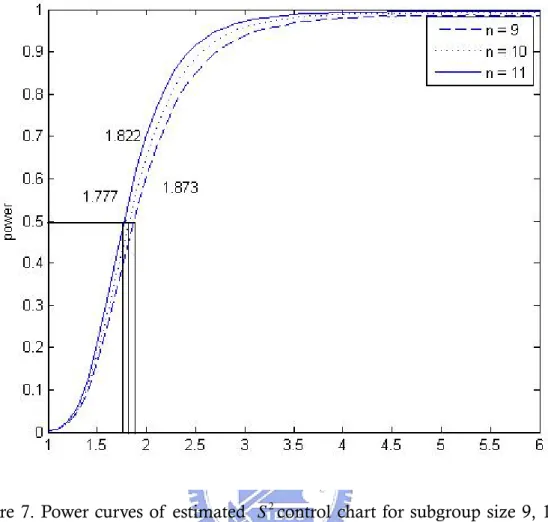
Figure 6. AS values with different α values. ...22 50 Figure 7. Power curves of estimated 2 S control chart for subgroup size 9, 10, and 11 when (α β, ) = (1,7). ...23
Figure 8. A view on common SMDs...25
Figure 9. Dimension of SMD...26
Figure 10. Histogram plot of the historical data. ...27
Figure 11. Weibull probability plot of the historical data...27
Chapter 1. Introduction
1.1. Research Background and Motivation
Process capability indices (PCIs) which provide numerical measure of production characteristic to reflect the quality of product have been used in the manufacturing industry. Those indices have become popular as unit-less measures on process potential and performance. The most commonly used ones, C and p
pk
C discussed in Kane (1986), and more-advanced indices Cpm and Cpmk
developed by Chan et al. (1988) and Pearn et al. (1992). Many authors have promoted the use of various PCIs for evaluating a supplier’s process capability. Based on analyzing the PCIs, a production department can trace and improve a poor process so that the quality level can be enhanced and the requirements of the customers can be satisfied. These PCIs have been defined explicitly as:
μ μ σ σ σ σ μ − ⎧ − − ⎫ − = = ⎨ ⎬ = ⎩ ⎭ 2+ − 2 , min , , 6 3 3 6 ( ) p pk pm
USL LSL USL LSL USL LSL
C C C T , μ μ σ μ σ μ ⎧ − − ⎫ ⎪ ⎪ = ⎨ ⎬ + − + − ⎪ ⎪ ⎩ 2 2 2 2 ⎭ min , , 3 ( ) 3 ( ) pmk USL LSL C T T
where USL is the upper specification limit, LSL is the lower specification limit,
μ is the process mean, σ is the process standard deviation, and T is the target value.
The first capability index C considers the overall process variability relative p
to the manufacturing tolerance, reflecting product quality consistency. Due to the design is simplicity, Cp can not reflect the tendency of process centering.
The index C was created in Japan to offset some of the weaknesses in pk
p
C , primarily because the fact that C measures capability in terms of process p
variation only and does not take process location into consideration. However,
pk
C considers process variation and the location of process mean. It has been
regarded as a yield-based index since it provides lower bounds on process yield, and is always used to measure the quality of the process. For example, when the
= 1
pk
C means that the product’s fractions of defectives is not more than 2700 parts per million (ppm) fall outside the specification limits. At Cpk = 1.33, the defect rate drops to 66 ppm. To achieve that defect rate less than 0.544 ppm, a
pk
C level of 1.67 is required. At a C level of 2.0, the defective rate reduced to pk
detect this movement obviously. So that the C will be underestimated the true pk
number of nonconformities. At the present time, the C index is used more pk
than any other index for measuring process capability. It is the reason why we study C more than other indices here. pk
Since Motorola, Inc. introduced its Six Sigma quality initiative, followers of this philosophy notion should add 1.5σ when estimating process capability. When asked the reason for such an adjustment, six-sigma user claim it is necessary, but offer only personal experiences and three dated empirical literature. Bothe (2002) provided a statistical reason to adjust the C be overestimated, and pk
he set the adjustment of shift in average that was dependent on the same detection power of the control chart, and the data of Bothe’s study was assumed to be approximately normality distribution. However effectively non-normal process occurs frequently in practice. Pyzdek (1995) has mentioned the distributions of certain chemical processes such as zinc plating thickness of a hot-dip galvanizing process are very quite often skewed. Choi (1996) presents an example of a skewed distribution in the ‘active area’ shaping stage of the wafer’s production process. Cygan et al. (1989) have mentioned that the lifetimes of polypropylene films under high ac and dc field stresses be shown as a two-parameter Weibull distribution. The Weibull distribution, denoted as Weibull (α β, ), with various values of scale parameter α and shape parameter β , covers a wide class of non-normal applications, including product life, product reliability and tensile strength of brittle materials, such as carbon and boron. The abundance of outputs from skewed distribution, the censoring, etc, makes the normality assumption often being illegitimate. Specifically, we assure the product lifetime which be from skewed distribution by statistic test and historical data. It will lead to underrate the probability of nonconformance that using the adjustment for normal case to adjust the non-normal cases.
1.2. Research Purpose
For some non-normal cases, Hsu et al. (2007) provided the process capability adjustment for gamma processes, and Li (2007) provided the process capability adjustment for Weibull processes, but they only investigate the change of the process mean shift. In real world, the process is dynamic, the mean and variance could change with small movement for momentary. In this thesis, we focus on the process variance change for non-normal cases.
We investigate Weibull distribution to calculate the ARL(average run length) by simulation. We also show the detection power performance of 2
S chart under
variance change. In the cases, we show that the detection power in this control chart is very sensitive. When the data are from Weibull distribution, we provide the statistical derived variance change adjustment based on the chart subgroup size and distribution parameter to calculate the estimate of dynamic C when pk
the data is non-normal distribution. It can make sure our process capability do not overestimate.
First, we introduce the research motivation and purpose in Chapter 1. Secondly, a brief introduction of Bothe’s study and adjustment reason for mesn shift are included, and adjustment for Weibull process is also in Chapter 2. In Chapter 3, we introduce the characteristic of Weibull distribution, and introduce some properties for S of Weibull process. Then, we compare the difference 2
between normal process and Weibull process on variance distribution. In chapter 4, we use the MATLAB program to create a Monte-Carlo simulation to find upper and lower control limits for detecting variance change. We provide the simulation derived adjustments based on the chart’s subgroup size (for Weibull distribution) to calculate the estimator of dynamic C when the data is Weibull pk
distribution. For illustrative purpose, application is presented in Chapter 5. Finally, we give some conclusion in Chapter 6.
Chapter 2. Literature Review
The process capability adjustment for mean shift for normal and non-normal distributions had been researched. In this section, we will review those papers about adjustments for normal process and Weibull process.
2.1. Process Capability Adjustment for Normal Process with Mean Shift
Bothe (2002) provided a statistical reason why to add a 1.5σ shift to the average. Assuming the processes approximately normal distribution, control charts can not reliably detect small movement in average. When μ had a small movement (ex: 0.5σ , 1σ ) and the detection power of Shewhart X control chart is too small to discover. Then, small mean movement affects the PCIs accuracy. However, the probability of nonconformance will increase obviously. For example, when Cpk is 1.33, the probability of nonconformance is 64 ppm. If
average occur 1σ shift that be difficultly detected by control chart, the probability of nonconformance becomes 1350 ppm. The probability of nonconformance will increase twenty-fold. Bothe considered that adjustments should accord with the same detection standard.
Bothe (2002) considered providing the same detection power in order to define the several adjustments with different subgroup size and called the adjustment S . By this idea, he set the detecting power to 50 percent and 50
computed the several adjustments for different subgroup size. The reason which Bothe set the power to 50 percent was we want detect the processes out of control immediately if the process mean shifts and the ARL (average run length)=1 is 1
the perfect condition. But in fact, the ARL = is impossible. For this reason we 1 1 can just only set the ARL = , and the detection power is 1 2 1 ARL , so we can 1
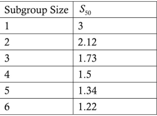
know if ARL = the detecting power is 0.5. The results showed in Table 1. 1 2 Table 1 displays shift sizes that have 50 percent chance of remaining undetected for subgroup sizes 1 through 6. Because shifts ranging in size from 0 up to S50σ
are the ones likely to remain undetected, a conservative approach is to assume that every missed shift is as large as S50σ . And Bothe invented dynamic Cpk be
defined as 50 50 ( ) ( ) min , . 3 3 pk USL S S LSL dynamic C μ σ μ σ σ σ − + − − ⎡ ⎤ = ⎢ ⎥ ⎣ ⎦
Bothe (2002) suggested that the adjustment value for normal distribution should be determined by the subgroup size n.
Table 1. Adjustment values for normal distribution with several subgroup size. Subgroup Size S 50 1 3 2 2.12 3 1.73 4 1.5 5 1.34 6 1.22
2.2. Process Capability Adjustment for Weibull Process with Mean Shift
Li (2007) provided the process capability adjustment for non-normal processes. Weibull distribution does not have reproductive property, and the distribution of the X distribution is analytically intractable. Lu (2003) provided to approximate the cumulative density function of X for Weibull processes. n
The UCL and LCL was set to 99.865th and 0.135th percentile of
n
X
distribution. We call the control chart they used as percentile Weibull control chart. Then, these two papers used the control limits to calculate the detection power for Weibull processes under various subgroup sizes n and shape parameter β.
Since the shape of the Weibull distribution changing from positive skewness to negative skewness with increasing the shape parameter, Li (2007) discussed two different cases. Process mean had right and left shifts. He used this cumulative density function to compute the relationship between the mean shift and Type Ⅱ error and calculate the mean shift adjustment AS50 which means that the
processes mean shift AS50σ when the detection power of control chart is 0.5.
Table 2. AS50 values for several nand various β values with mean right shift.
50
AS Weibull distribution(1,β) for right shift
n 1 2 3 4 5 6 7 8 9 10 2 3.611 2.492 2.009 1.767 1.632 1.536 1.470 1.424 1.387 1.359 3 2.735 1.967 1.642 1.482 1.373 1.307 1.261 1.228 1.197 1.182 4 2.250 1.663 1.448 1.309 1.232 1.175 1.138 1.103 1.087 1.071 5 1.944 1.484 1.301 1.196 1.127 1.084 1.047 1.025 1.006 0.988 6 1.716 1.343 1.201 1.104 1.043 1.009 0.981 0.960 0.942 0.932 7 1.569 1.239 1.119 1.037 0.990 0.954 0.928 0.907 0.892 0.881 8 1.440 1.159 1.051 0.984 0.939 0.905 0.883 0.864 0.852 0.839 9 1.340 1.086 0.991 0.930 0.891 0.865 0.845 0.828 0.814 0.805 10 1.251 1.031 0.943 0.889 0.853 0.828 0.811 0.797 0.784 0.773
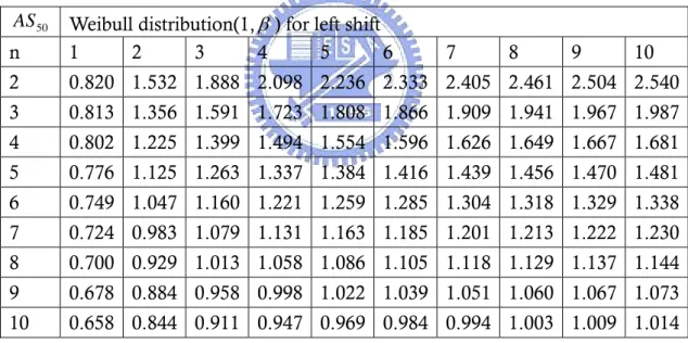
Table 3. AS50 values for several nand various β values with mean left shift.
50
AS Weibull distribution(1,β) for left shift
n 1 2 3 4 5 6 7 8 9 10 2 0.820 1.532 1.888 2.098 2.236 2.333 2.405 2.461 2.504 2.540 3 0.813 1.356 1.591 1.723 1.808 1.866 1.909 1.941 1.967 1.987 4 0.802 1.225 1.399 1.494 1.554 1.596 1.626 1.649 1.667 1.681 5 0.776 1.125 1.263 1.337 1.384 1.416 1.439 1.456 1.470 1.481 6 0.749 1.047 1.160 1.221 1.259 1.285 1.304 1.318 1.329 1.338 7 0.724 0.983 1.079 1.131 1.163 1.185 1.201 1.213 1.222 1.230 8 0.700 0.929 1.013 1.058 1.086 1.105 1.118 1.129 1.137 1.144 9 0.678 0.884 0.958 0.998 1.022 1.039 1.051 1.060 1.067 1.073 10 0.658 0.844 0.911 0.947 0.969 0.984 0.994 1.003 1.009 1.014
Table 2 and Table 3 display the magnitude of mean shift adjustments AS50
based on the detection power set to 0.5 and data from Weibull (1, β ) distribution for various value of β = 1(1)10 and n=2(1)10 with right shift (k >0) and left shift
(k <0). They also used the most common method for modifying PCIs in the
non-normal case is the technique of quantile estimation, and the dynamic C pk
was as the same as gamma processes which Hsu et al. (2007) provided.
Noting that a process will experience shifts in X0.50(median) of various
magnitudes and knowing that not all of these will be discovered, some allowance for them must be made when estimating outgoing quality so customers are not
disappointed. Because shifts ranging in size from 0 up to AS50σ are likely to
remain undetected, a conservative approach it to assume that every missed shift it as large as AS50. When estimating capability, X0.5 minus AS50σ is used to
evaluate how well the process output meets the LSL and X0.5 plus AS50σ is
used for determining conformance to the USL. Both of these adjustments are incorporated into the Cpk formula, now called the “dynamic” Cpk index, by
making the following modifications:
0.5 50 0.5 50 0.5 0.135 99.865 0.5 0.5 50 0.5 50 0.5 0.135 99.865 0.5 ( ) LSL USL ( ) min{ , } LSL USL min{ , } pk X AS X AS dynamic C X X X X X AS X AS X X X X σ σ σ σ − − − + = − − − − − − = − −
The capabability adjustments for Weibull processes are related to which control chart chosen to control the process. The Shwehart X control chart assumes that the process data come from a normal or near-normal distribution. When the data comes from Weibull distribution, we should choose control charts for non-normal processes or for Weibull processes to control production process. Padgett and Supurrier (1990) used Monte Carlo simulation to construct Shewhart-type control charts for percentiles of strength distributions. Chan and Cui (2003) provided a skewness correction X and R charts for skewed distributions. This control chart proposed a skewness correction method for constructing the X and R control charts for skewed process distributions. Their asymmetric control limits are based on the degree of skewness estimated from the subgroups. Nichols and Padgett (2006) provided a bootstrap Weibull control chart. This control chart use bootstrap method to simulate the UCL
and LCL for monitoring Weibull percentiles. Erto (2007) provided a Weibull control chart which used Bayes theorem to calculate the sampling distribution of Weibull percentile.
Lu (2008) considered the problem of how to determine the adjustments for process capability with mean shift when data follows the Weibull distribution. Lu (2008) compared the detection powers of the percentile Weibull control chart, bootstrap Weibull control chart and the Erto’s Weibull control chart under the Bothe’s adjustments, and showed the Bothe’s adjustments are inadequate when data come from Weibull processes. He finds the Erto’s Weibull control chart is the best powerful control chart than the others. For Weibull processes, Lu (2008) calculated the adjustments for various sample sizes (n) and Weibull shape parameter (β) with detection power of the Erto’s Weibull control chart fixed to 0.5. Using the adjusted process capability formula, the engineers can determine the actual process capability more accurately.
Chapter 3. Investigation for Weibull Process
In this section, we introduce the characteristic of Weibull distribution first. In the second part, we investigate the Weibull variance distribution to study the effect on the detection power of the 2
S control chart.
3.1. Weibull Process
The Weibull distribution has been widely used in the field of life data analysis due to its flexibility. It has similar behavior of other statistical distributions such as normal and the exponential distributions. The Weibull distributions are also used to model the time until a given technical device fails. In practical, the Weibull has been used include electronic devices such as memory element, mechanical components such as bearings, and structural elements in aircraft and automobiles,...,etc. The Weibull distribution can also be used to model the distribution of wind speeds at a given location on Earth. Moreover, every location is characterized by a particular shape and scale parameter.
If the failure rate of the device decreases over time, one choosesβ <1 (β is the shape parameter). If the failure rate of the device is constant over time, one choosesβ =1, again resulting in a decreasing function f. If the failure rate of the device increases over time, one chooses β >1 and obtains a density f which increases towards a maximum and then always decreases.
In this thesis, we consider Weibull distribution as the process population to study the effect on the capability estimates when the process output has a non-normal distribution with process variance change. Observations from the Weibull distribution is non-negative. The Weibull distribution can be denoted as Weibull (α,β ) with cumulative density function and the probability density function given by ( / ) ( ) 1 e x , 0, X F x = − − αβ x≥ and ( ) 1 ( ) , 0, x f x x e x β β β α βα− − − = ≥
where ( 0)α > is the scale parameter, and ( 0)β > is the shape parameter. The mean and variance of Weibull distribution are
1 [ (1 )], μ α= Γ +β− and 2 2 1 2 1 [ (1 2 ) (1 )]. σ =α Γ + β− − Γ +β−
The Weibull distribution is very flexible, and by appropriate selection of the parameters α and β , we can obtain a various shapes. Since the Weibull distribution is skewed, we utilize the coefficient of skewness and kurtosis to explain how this distribution is different from normal distribution, the coefficient of skewness and kurtosis of Weibull distribution can be expressed as follows:
3 1 1 1 1 1 1 2 1 3/ 2 2 (1 ) 3 (1 ) (1 2 ) (1 3 ) , [ (1 2 ) (1 )] β β β β γ β β − − − − − − Γ + − Γ + Γ + + Γ + = Γ + − Γ + and 2 1 2 1 2 ( ) , [ (1 2 ) (1 )] β γ β− β− = Γ + − Γ + f
where Γ(x) is the gamma function and
4 1 2 1 1 2 1 1 1 1 ( ) 6 (1 ) 12 (1 ) (1 2 ) 3 (1 2 ) 4 (1 ) (1 3 ) (1 4 ). f β β β β β β β β − − − − − − − ≡ − Γ + + Γ + Γ + − Γ + − Γ + Γ + + Γ +
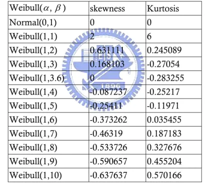
Table 4 presents the coefficient of skewness and the coefficient of kurtosis of the Weibull distribution under study.
Table 4. Values of skewness and kurtosis of various Weibull distributions. Weibull(α β, ) skewness Kurtosis
Normal(0,1) 0 0 Weibull(1,1) 2 6 Weibull(1,2) 0.631111 0.245089 Weibull(1,3) 0.168103 -0.27054 Weibull(1,3.6) 0 -0.283255 Weibull(1,4) -0.087237 -0.25217 Weibull(1,5) -0.25411 -0.11971 Weibull(1,6) -0.373262 0.035455 Weibull(1,7) -0.46319 0.187183 Weibull(1,8) -0.533726 0.327676 Weibull(1,9) -0.590657 0.455204 Weibull(1,10) -0.637637 0.570166
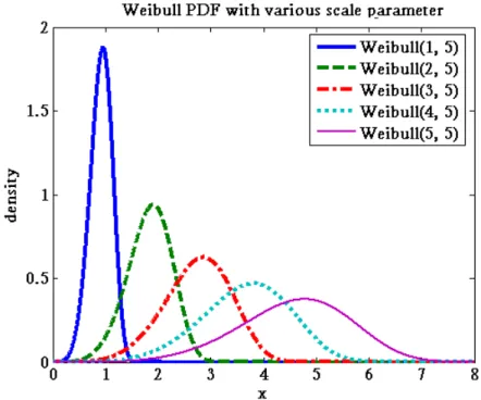
Figure 1 shows the plot of probability density function of Weibull distribution with various values of α , while β is fixed. From Figure 1, we can find the scale parameter only control the mean and the variance to adjust the shape of the distribution. Figure 2 presents Weibull distribution with variousβ, while α is fixed. In Figure 3, we observed that the Weibull distribution is more similar to normal distribution while the shape parameter β exceeds 2. From
Figure 1. Weibull distribution with various α .
Figure 2. Weibull distribution with various β
-10 -5 0 5 10 15 0 0.2 0.4 0.6 0.8 1 1.2 1.4 1.6 1.8 2 x dens it y
PDF for Weibull(1,0.5) and Normal(2,20)
-3 -2 -1 0 1 2 3 4 5 0 0.2 0.4 0.6 0.8 1 1.2 1.4 1.6 1.8 2
PDF for Weibull(1,1) and N(1,1)
x
de
ns
it
y
Figure 3(a). Probability density functions for Weibull(1,0.5) along with a Normal distribution.
Figure 3(b). Probability density functions for Weibull(1,1) along with a Normal distribution.
-0.50 0 0.5 1 1.5 2 2.5 0.2 0.4 0.6 0.8 1 1.2 1.4 1.6 1.8 2
PDF for Weibull(1,2) and N(0.886, 0.214)
x de ns it y -0.50 0 0.5 1 1.5 2 2.5 0.2 0.4 0.6 0.8 1 1.2 1.4 1.6 1.8 2 x de ns it y
PDF for Weibull(1,3) and N(0.892, 0.105)
Figure 3(c). Probability density functions for Weibull(1,2) along with a Normal distribution.
Figure 3(d). Probability density functions for Weibull(1,3) along with a Normal distribution.
-0.50 0 0.5 1 1.5 2 2.5 0.2 0.4 0.6 0.8 1 1.2 1.4 1.6 1.8 2
PDF for Weibull(1,4) and N(0.906, 0.0647)
x dens it y -0.50 0 0.5 1 1.5 2 2.5 0.2 0.4 0.6 0.8 1 1.2 1.4 1.6 1.8 2
PDF for Weibull(1,5) and N(0.9181, 0.0442)
x
de
ns
it
y
Figure 3(e). Probability density functions for Weibull(1,4) along with a Normal distribution.
Figure 3(f). Probability density functions for Weibull(1,5) along with a Normal distribution.
0 0.2 0.4 0.6 0.8 1 1.2 1.4 1.6 1.8 2 0 0.5 1 1.5 2 2.5 3 3.5 4
PDF for Weibull(1,9) and N(0.947, 0.0158)
x d ens it y 0 0.2 0.4 0.6 0.8 1 1.2 1.4 1.6 1.8 2 0 0.5 1 1.5 2 2.5 3 3.5 4
PDF for Weibull(1,10) and N(0.951, 0.013)
x
dens
it
y
Figure 3(g). Probability density functions for Weibull(1,9) along with a Normal distribution.
Figure 3(h). Probability density functions for Weibull(1,10) along with a Normal distribution.
Figure 3(a)-3(h). Probability density functions for Weibull distributions along with a Normal distribution for the same mean and variance. Let β = 0.5, 1, 2, 3, 4, 5, 9, and 10.
3.2. Sampling Distribution of Sample Variance for Weibull Process
Because the sampling distribution of variance for Weibull process is difficult to find, so we use the Matlab program to generate 1,000,000 preliminary samples from Weibull( ,α β ), each of size k, and let Si be the variance of the ith sample
to simulate the empirical distribution. We want to know about the distribution when shape parameter changed for Weibull distribution. In Figure 4, we draw several empirical probability density functions of the sample variance when data come from Weibull and normal populations having the same mean and variance, we let β = 0.5, 1, 2, 3, 4, 5, 6, 7, 8, and 9. The sample size is set to be 11. We can find the empirical sampling distribution of variance as below:
Figure 4(a). Empirical distribution of sample variance for Weibull(1,0.5) and Normal(2,20).
Figure 4(b). Empirical distribution of sample variance for Weibull(1,1) and Normal(1,1).
Figure 4(c). Empirical distribution of sample variance for Weibull(1,2) and Normal(0.8862,0.2146).
Figure 4(d). Empirical distribution of sample variance for Weibull(1,3) and Normal(0.893,0.1053).
Figure 4(e). Empirical distribution of sample variance for Weibull(1,4) and Normal(0.9064,0.0674).
Figure 4(f). Empirical distribution of sample variance for Weibull(1,5) and Normal(0.9182,0.0442).
Figure 4(i). Empirical distribution of sample variance for eibull(1,8) and Normal(0.9417,0.0195).
Figure 4(j). Empirical distribution of sample variance for Weibull(1,9) and Normal(0.947,0.0158 ).
Figure 4(a)-4(j). Empirical distribution of sample variance for Weibull distribution along with Normal distribution on the same mean and variance.
It follows from Figure 3 that when the shape parameter is larger than 2, the Weibull distribution appears to be near normal distribution. So we can infer that the sampling distribution of variance from Weibull distribution is close to the sampling distribution of variance from normal population when β is larger than 2. This phenomenon can be verified from the simulation result shown in Figure4. Moreover, From Figure 4 we also observe that as β is smaller than 2, the tail will be more elongate (distribution is strongly skewed). In Figure 5, we draw several empirical sampling distribution of variance for Weibull withβ = 0.5, 0.7, 0.9, 1.1, 1.3, 1.5, 1.7, and 1.9 , and sample size = 11.
Figure 5(a). Empirical distribution of sample variance for Weibull(1,0.5).
Figure 5(b). Empirical distribution of sample variance for Weibull(1,0.7).
Figure 5(a). Empirical distribution of sample variance for Weibull(1,0.9).
Figure 5(b). Empirical distribution of sample variance for Weibull(1,1.1).
Figure 5(b). Empirical distribution of sample variance for Weibull(1,1.3).
Figure 5(b). Empirical distribution of sample variance for Weibull(1,1.5).
Chapter 4. Process Variance Change Investigation for
Weibull Process
In this chapter, we introduce a percentile control chart to investigate the detection power for the process variance change. Then we use it to find the modified standard deviation adjustment for Weibull process.
4.1. Average Run Length
ARL of the control chart means the average number of points that must be poltted before a point indicates an out-of-control condition. If the process observations have some problems, the ARL can be calculated as below:
ARL=1 p,
where p means the probability of any point exceeds the control limits.
There are two kinds of ARL for any Shewhart control chart. The first one we can be expressed as ARL for the in-control ARL. It means that the process 0 observations are corrected, but there will be an out of control single generated every ARL samples, on average. We can easily calculate as below: 0
ARL =0 1
α ,
where α is the probability of indicating a shift when none has occurred.
The second one for the out-of-control ARL can be also be expressed as
1
ARL . It means the process observations are uncorrected, so we will find out the out of control single generated every ARL samples, on average. It can be 1 calculated as below:
ARL =1 1 1−β ,
where β is the probability of failing to indicate a real shift in process level. In this paper, we will use the ARL to find the modified standard deviation 1 adjustment for Weibull process, then we can use it to modify our process capability index C . pk
4.2. Monte-Carlo Simulation for Determining UCL and LCL
The main purpose of individuals control chart is assisting on identifying shifts or drifts in processes and it’s easily to be implemented. In this paper we study the effects on the capability estimates when the process output obeys gamma distribution with process variance change is remained unknown, so the
2
S control chart is a convention tool to monitor process variability and can help
us quickly determine whether the process is stable or not. But, when we adopt the control chart, some assumptions should be satisfied, such as the process characteristics must follow normal distribution. However, since our study is based on the gamma processes, violating the assumption, we will need to replace the traditional upper and lower control limits,
(
2)
22, 1
1 n
S n− χα − and
(
S n2 −1)
χ12−(α2 , 1)n− , as quantiles of the cumulative distribution function fromdifferent parameters of Weibull(α β, ), where S is an unbiased estimator of 2 σ2.
In order to calculate the probability of misjudgment, one will first need to know the upper and lower control limits (UCL and LCL, respectively) of the process run. It is extremely difficult, if not impossible, to obtain the explicit formula of the distribution of sample variance when data follow gamma distribution. In this paper, Monte-Carlo simulation method was performed to investigate the behavior of sampling distribution of variance for gamma data and determine the estimated upper and lower control limits. So, in our study, the
UCL and LCL are estimated through Monte-Carlo simulation method. The steps of Monte-Carlo algorithm to determine the control limits of S control 2
chart are summarized as follows:
Step1: We generate N preliminary samples from Weibull(α ,β), each of size k, and let Si be the variance of the ith sample.
Step2: To sort S , we obtain i S <S <...<S , let (1) (2) (N) ˆtp be the percentile for S . i
For example N=10 , then ˆ6
6
0.1 (10 )
t =S , so ˆt =Sp (N*p).
Step3: The upper and lower control limits for Weibull(α ,β) can be estimated by ˆt0.99865and ˆt0.00135.
4.3. Detection Power of S for Weibull Data 2
Utilizing the UCL and LCL obtained by Monte-Carlo approach, we derived the power of S for Weibull process data. Since the Type II error 2 β is
(
)
empirical cumulative distribution function of sample variance from Weibull distribution with that variance has changed and σ1 is the standard deviation
after process change ( σ0 is the standard deviation of the original process). The control limits LCL and UCL are calculated as F0.00135 and F0.99865
respectively.
We develop a Matlab program to compute the probability of process variance out of control limits. When process variance changes from σ2to k2×σ2, and
mean is fixed, the parameters α and β will change to new parameters '
α and 'β , then we can obtain the detection power under the situation that the process variance changes. The parameters α and '' β can be found by untilizing the following steps:
Step1: Assume the new standard deviation σ1= × , and k,k σ μ,andσ are all
known.
Step2: The mean and variance of Weibull distribution are 1
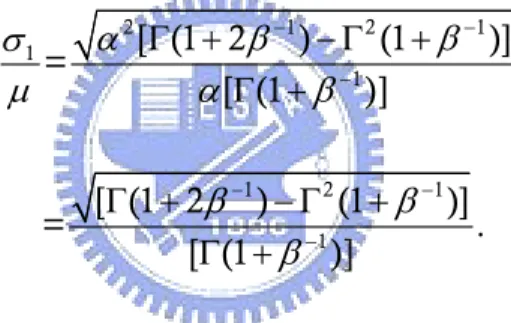
[ (1 )] μ α= Γ +β− and 2 2 1 2 1 [ (1 2 ) (1 )]. σ =α Γ + β− − Γ +β− Then, we compute 1 σ divided by μ as below: α β β σ μ α β − − − Γ + − Γ + Γ + 2 1 2 1 1 1 [ (1 2 ) (1 )] = [ (1 )] β β β − − − Γ + − Γ + Γ + 1 2 1 1 [ (1 2 ) (1 )] = . [ (1 )]
Step3: We can find the new scale and shape parameters α and '' β .
Table 5 displays the detection power when data come from Weibull distribution with α =1 and β =3, 4, and 5. The change magnitude is 1.0(0.5)3.5 adjustments. From Table 5, we observe the detection power gets larger as sample size (n) increasing.
Table 5. Detection power for various weibull distributions. Weibull(1,3) Subgroup Size n Magnitude of change in σ 9 10 11 12 13 1 0.00272 0.00286 0.00268 0.00266 0.00276 1.5 0.23732 0.26349 0.28855 0.31660 0.34155 2 0.58041 0.62368 0.66314 0.70087 0.73517 2.5 0.72655 0.76466 0.80016 0.83068 0.85645
3 0.78041 0.81628 0.84627 0.87217 0.89399 3.5 0.80037 0.83348 0.86098 0.88494 0.90451 Weibull(1,4) Subgroup Size n Magnitude of change in σ 9 10 11 12 13 1 0.00264 0.00277 0.00259 0.00273 0.00275 1.5 0.23987 0.27072 0.29748 0.32572 0.35763 2 0.64447 0.69275 0.73354 0.77036 0.80625 2.5 0.81486 0.85297 0.88250 0.90716 0.92722 3 0.87588 0.90519 0.92758 0.94490 0.95854 3.5 0.89843 0.92341 0.94229 0.95637 0.96773 Weibull(1,5) Subgroup Size n Magnitude of change in σ 9 10 11 12 13 1 0.00262 0.00261 0.00267 0.00271 0.00275 1.5 0.21636 0.24175 0.27207 0.29781 0.32945 2 0.65080 0.69954 0.74586 0.78218 0.81768 2.5 0.84854 0.88345 0.91227 0.93255 0.95023 3 0.91675 0.93968 0.95792 0.97026 0.97916 3.5 0.94173 0.95917 0.97233 0.98074 0.98706
4.4. Modified Standard Deviation Adjustment for Weibull Process
We set a given sample size (n) α =1 and given β, then sampling large data ( 7
10 ) which are from Weibull distribution to estimate the control limits and compute the detection power of S for Weibull data with the given change 2
magnitude and n.
From the mentioned above, we fix power =
(
≤ 2 ≤ σ = σ)
1 0
|
P LCL S UCL k = 0.5 to find k. We develop a Matlab program to compute the standard deviation change adjustment AS . The standard deviation adjustment means that
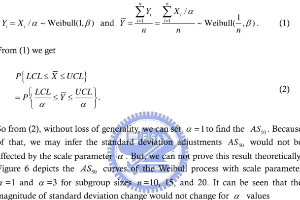
of =β 1(1)11 and n=8(1)35. For example, if β is 3 with n=10, the standard deviation change adjustment AS50 is 1.785. When β=1, AS50 are all greater
than 5. From Figure 4, we find the shape is extraordinarily unlike the normal distribution when β=1.When shape parameter is smaller than 1.5 (see Figure 5), we note that thedistribution is a long-tail right skewed distribution.
Why not discuss the relationship between AS50 and scale parameter α ?By
Lu (2003), we can compute the probability of Xn when X1,...,Xn is a random
sample from Weibull( ,α β ), and if we let Yi =Xi/α then we have
/ ~ Weibull(1, ) i i Y = X α β and 1 1 / 1 ~ Weibull( , ) n n i i i i Y X Y n n n α β = = =
∑
=∑
. (1) From (1) we get{
}
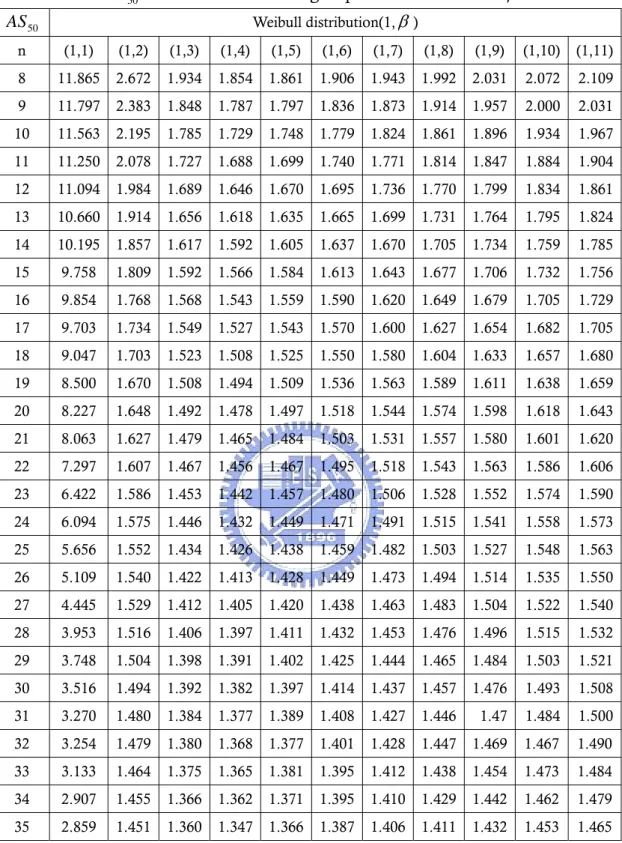
. P LCL X UCL LCL UCL P Y α α ≤ ≤ ⎧ ⎫ = ⎨ ≤ ≤ ⎬ ⎩ ⎭ (2)So from (2), without loss of generality, we can set α =1to find the AS50. Because
of that, we may infer the standard deviation adjustments AS50 would not be
affected by the scale parameter α . But, we can not prove this result theoretically. Figure 6 depicts the AS curves of the Weibull process with scale parameter 50
α =1 and α =3 for subgroup sizes n=10, 15, and 20. It can be seen that the magnitude of standard deviation change would not change for α values
Table 6. AS50 values for several subgroup size n and various β values. 50 AS Weibull distribution(1,β) n (1,1) (1,2) (1,3) (1,4) (1,5) (1,6) (1,7) (1,8) (1,9) (1,10) (1,11) 8 11.865 2.672 1.934 1.854 1.861 1.906 1.943 1.992 2.031 2.072 2.109 9 11.797 2.383 1.848 1.787 1.797 1.836 1.873 1.914 1.957 2.000 2.031 10 11.563 2.195 1.785 1.729 1.748 1.779 1.824 1.861 1.896 1.934 1.967 11 11.250 2.078 1.727 1.688 1.699 1.740 1.771 1.814 1.847 1.884 1.904 12 11.094 1.984 1.689 1.646 1.670 1.695 1.736 1.770 1.799 1.834 1.861 13 10.660 1.914 1.656 1.618 1.635 1.665 1.699 1.731 1.764 1.795 1.824 14 10.195 1.857 1.617 1.592 1.605 1.637 1.670 1.705 1.734 1.759 1.785 15 9.758 1.809 1.592 1.566 1.584 1.613 1.643 1.677 1.706 1.732 1.756 16 9.854 1.768 1.568 1.543 1.559 1.590 1.620 1.649 1.679 1.705 1.729 17 9.703 1.734 1.549 1.527 1.543 1.570 1.600 1.627 1.654 1.682 1.705 18 9.047 1.703 1.523 1.508 1.525 1.550 1.580 1.604 1.633 1.657 1.680 19 8.500 1.670 1.508 1.494 1.509 1.536 1.563 1.589 1.611 1.638 1.659 20 8.227 1.648 1.492 1.478 1.497 1.518 1.544 1.574 1.598 1.618 1.643 21 8.063 1.627 1.479 1.465 1.484 1.503 1.531 1.557 1.580 1.601 1.620 22 7.297 1.607 1.467 1.456 1.467 1.495 1.518 1.543 1.563 1.586 1.606 23 6.422 1.586 1.453 1.442 1.457 1.480 1.506 1.528 1.552 1.574 1.590 24 6.094 1.575 1.446 1.432 1.449 1.471 1.491 1.515 1.541 1.558 1.573 25 5.656 1.552 1.434 1.426 1.438 1.459 1.482 1.503 1.527 1.548 1.563 26 5.109 1.540 1.422 1.413 1.428 1.449 1.473 1.494 1.514 1.535 1.550 27 4.445 1.529 1.412 1.405 1.420 1.438 1.463 1.483 1.504 1.522 1.540 28 3.953 1.516 1.406 1.397 1.411 1.432 1.453 1.476 1.496 1.515 1.532 29 3.748 1.504 1.398 1.391 1.402 1.425 1.444 1.465 1.484 1.503 1.521 30 3.516 1.494 1.392 1.382 1.397 1.414 1.437 1.457 1.476 1.493 1.508 31 3.270 1.480 1.384 1.377 1.389 1.408 1.427 1.446 1.47 1.484 1.500 32 3.254 1.479 1.380 1.368 1.377 1.401 1.428 1.447 1.469 1.467 1.490 33 3.133 1.464 1.375 1.365 1.381 1.395 1.412 1.438 1.454 1.473 1.484 34 2.907 1.455 1.366 1.362 1.371 1.395 1.410 1.429 1.442 1.462 1.479 35 2.859 1.451 1.360 1.347 1.366 1.387 1.406 1.411 1.432 1.453 1.465
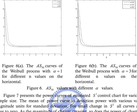
Figure 7 presents the power curves of estimated 2
S control chart for various
sample size. The mean of power curve is detection power with various vary magnitude units for standard deviation. For small change in S all curves are 2
close to zero. As the magnitude of change creasing, so does the power of chart to detect it. The horizontal line drawn on this graph shows that is a 50% chance of missing a 1.777 times the size of standard deviation when n is 11, where as σ
must change 1.873 times to have this same probability when n is 9.
Figure 6(a). The AS curves of 50
the Weibull process with α =1 for different n values on the horizontal.
Figure 6(b). The AS curves of 50
the Weibull process with α =3for different n values on the horizontal.
Figure 7. Power curves of estimated 2
S control chart for subgroup size 9, 10, and
11 when (α β, ) = (1,7).
4.5. Capability Adjustment for Weibull Process
The index Cpk has been referred to as a yield-based index since it provides
bound on the process on the process yield for a normality distribution process with a fixed value of Cpk.This index Cpk is defined in chapter 1. The proper use
of process capability, is based on several assumptions. One of the most important assumption is that the process monitored is supposed to be stable and the output is approximately normal distribution.
When the distribution of a process characteristic is non-normal, PCIs calculated using existing method often lead to erroneous and misleading interpretation of the process capability. Several approaches to the problems of PCIs for the non-normal populations have been suggested. Chen and Pearn (1997) consider come generalizations of these basic capability indices to cover non-normal distribution. In the non-normal case, if we are able to find a better
0.5 0.99865 0.5 pu USL X C X X − = − , and pl 0.50.5 0.00135 X LSL C X X − = −
The index Cpk will then be calculated as the minimum of Cpu and Cpl,
namely: Cpk =min
{
C Cpu, pl}
0.5 0.5 0.99865 0.5 0.5 0.00135 min USL X , X LSL X X X X ⎧ − − ⎫ = ⎨ ⎬ − − ⎩ ⎭Acknowledging that a process will experience change in X0.99865−X0.5 or
0.5 0.00135
X −X of various magnitudes and knowing that not all of these will be discovered, some allowance for them must be made when estimating outgoing quality so customers are not disappointed. Because change ranging in times from 0 up to AS are the likely to remain undetected, a conservative approach it to 50
assume that every missed change it as large as AS50.
When utilizing dynamic Cpk to estimate process capability, we replace
0.99865 0.5 and 0.5 0.00135
X −X X −X withAS50(X0.99865−X0.5) and AS X( 0.5−X0.00135)in the
pk
C formula just mentioned above, respective. Both of these adjustments are
incorporated into the Cpk formula, now called the “dynamic” Cpk index, by
making the following modifications:
Dynamic 0.5 0.5 50 0.5 0.00135 50 0.99865 0.5 LSL USL min{ , } ( ) ( ) − − = − − pk X X C AS X X AS X X 0.5 0.5 50 0.5 50 0.00135 50 0.99865 50 0.5 LSL USL min{ − , − } = ⋅ − ⋅ ⋅ − ⋅ X X AS X AS X AS X AS X
By including the adjustment in this assessment for undetected variance change, the estimate of capability decreases and the number nonconforming parts measured (calculated) will increase.
Chapter 5. Application
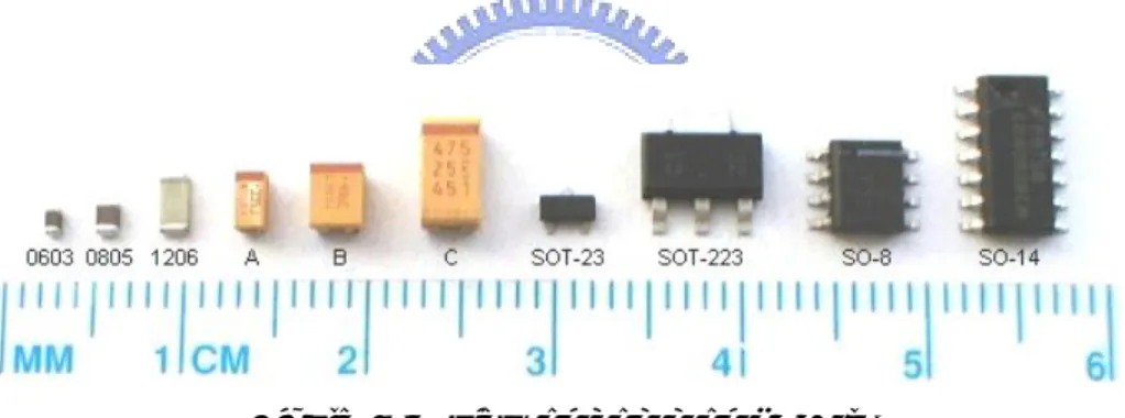
Surface-mount technology (SMT) is a method for constructing electronic circuits in which the components (SMC, or Surface Mounted Components) are mounted directly onto the surface of printed circuit boards (PCBs). Electronic devices so made are called surface-mount devices or SMDs. In the industry it has largely replaced the through-hole technology construction method of fitting components with wire leads into holes in the circuit board.
An SMT component is usually smaller than its through-hole counterpart because it has either smaller leads or no leads at all. It may have short pins or leads of various styles, flat contacts, a matrix of solder balls (BGAs), or terminations on the body of the component.
The SMD resistors come into several possible case sizes. Each size is described as a 4 digits number. The first 2 digits indicate the length; the last 2 indicate the width (in 0.01", or 10 mils units).Figure 9 display a view on common SMDs.For example, the three most popular sizes are “0603”, “0805”, and “1206”. That mean 1.6×0.3mm, 1.8×0.5mm, and 11.2×0.6mm.
Figure 8. A view on common SMDs.
At SMT process, one of the most important factors is the size of the SMD. The SMD resistor “0603” as shown in figure 9, we let the LSL and USL of the length for line segment “H” are 0.1mm and 0.5mm. This company utilize
2
S control chart to monitor the process. Generally, S2charts are preferable to
their more familiar counterparts, x−R charts, when either
1. The sample size n is moderately large-say, n>10or12. 2. The sample size n is variable.
Figure 9. Dimension of SMD.
This company use n=10 to monitor the process. The collected sample data
(a part of historical data) are shown in Table 7. From Figure 10, we use Minitab program to conclude the data collected from the factory are not normal distributed. The data analysis results justify that the process is significantly away from the normal distribution. By the goodness-of-fit tests as shown in figure 11, the historical data indicates that the process pretty approximates to be distributed as Weibull distribution. The parameters α and β of this Weibull process could be estimated from the historical data, giving αˆ 0.304= and βˆ 6.299 by MLE = (maximum likelihood estimate)
ˆ 1/ ˆ 1 1 ˆ n i i X n β β α = ⎡ ⎤ = ⎢⎣
∑
⎥⎦ , (2) and ˆ 1 ˆ 1 1 ln 1 1 ln ˆ n i i n i i n i i i X X X n X β β β = = = =∑
−∑
∑
. (3)Using the maximum likelihood Equations (2) and (3), we can estimateβ and α parameter when data are from Weibull distribution with the samples. Then we use the bootstrap to compute confidence intervals for shape parameter.
data Fr e q ue nc y 0.40 0.35 0.30 0.25 0.20 0.15 20 15 10 5 0 Mean 0.2828 StDev 0.05199 N 100 Histogram of data Normal
Figure 10. Histogram plot of the historical data.
C1 Pe rc e n t 0.40 0.30 0.20 0.15 0.10 0.09 0.08 99.9 99 90 80 70 60 50 40 30 20 10 5 3 2 1 0.1 Shape >0.250 6.299 Scale 0.3040 N 100 AD 0.215 P-Value Probability Plot of C1 Weibull - 95% CI
Figure 11. Weibull probability plot of the historical data. Table 7. The 100 observations are collected from the historical data. 0.1795 0.2641 0.2689 0.3114 0.3333 0.2827 0.3735 0.2584 0.3206 0.2433 0.2018 0.3194 0.259 0.3329 0.2876 0.2795 0.2866 0.1837 0.3523 0.3727 0.3154 0.2916 0.3195 0.2989 0.2545 0.3281 0.2697 0.2405 0.3196 0.3498 0.3191 0.2816 0.2758 0.2636 0.3037 0.2802 0.3008 0.3152 0.2396 0.2844 0.3018 0.2514 0.3949 0.2572 0.3235 0.3631 0.3398 0.2659 0.2357 0.2052 0.3122 0.3035 0.2447 0.3932 0.3259 0.31 0.3268 0.2792 0.3152 0.2646
We utilize this control chart to monitor the process, and collect another new dara are shown in Table 8. By the goodness-of-fit tests as shown in figure 12, the new data indicates that the process pretty approximates to be distributed as Weibull distribution. The parameters α and β of this Weibull process could be estimated from the historical data, giving αˆ 0.3041= and βˆ 0.5677 by MLE. =
C2 Pe rc e n t 0.50 0.40 0.30 0.20 0.15 0.10 0.09 0.08 0.07 99.9 99 90 80 70 60 50 40 30 20 10 5 3 2 1 0.1 Shape >0.250 5.677 Scale 0.3041 N 100 AD 0.295 P-Value Probability Plot of C2 Weibull - 95% CI
Figure 12. Weibull probability plot of the new data. Table 8. The 100 observations of the new data.
0.3114 0.2577 0.3851 0.2976 0.2509 0.2785 0.2032 0.2085 0.3123 0.2167 0.2172 0.2125 0.3085 0.2436 0.3209 0.2847 0.297 0.159 0.3274 0.2532 0.2908 0.2597 0.2209 0.2545 0.3907 0.272 0.2348 0.3345 0.2425 0.2379 0.2448 0.3157 0.3358 0.1581 0.3013 0.2311 0.2884 0.3055 0.1951 0.3037 0.1431 0.3473 0.2516 0.3034 0.2848 0.2636 0.3981 0.307 0.4135 0.2855 0.3433 0.3175 0.2944 0.3351 0.1861 0.3503 0.2198 0.2506 0.3348 0.2551 0.2448 0.3551 0.308 0.2301 0.1826 0.3463 0.2598 0.3072 0.3279 0.2644 0.1497 0.2452 0.383 0.2449 0.3383 0.3208 0.3235 0.2054 0.3257 0.2866 0.3644 0.3269 0.286 0.2341 0.2872 0.2883 0.2513 0.3035 0.347 0.3135 0.2634 0.2871 0.33 0.3247 0.2325 0.3333 0.3359 0.1721 0.3007 0.2539
Therefore, it is appropriate to use this approach and we can obtain more accurate measures of three quantile: X0.00135 =0.102105, X0.5 =0.282017, and
=
0.99865 0.411047
X under consideration. Then “dynamic” Cpk index can be calculate as follows:
0.5 0.5 50 0.99865 0.5 50 0.5 0.00135 USL LSL dynamic min , ( ) ( ) 0.5 281962 0.281962 0.1 min , 1.779 (0.411047 0.281962) 1.779 (0.281962 0.102105) pk X X C AS X X AS X X ⎧ − − ⎫ = ⎨ ⎬ − − ⎩ ⎭ ⎧ − − ⎫ = ⎨ ⎬ × − × − ⎩ ⎭ =min 0.949468,0.5687
{
}
=0.5687,with AS =1.779 for n=10 from Table 6. Compared it to the value of the 50
following index:
{
}
0.5 0.5 0.99865 0.5 0.5 0.00135 USL LSL min , 0.5 0.281962 0.281962 0.1 min , 0.411047 0.281962 0.281962 0.102105 min 1.6891,1.0117 1.0117, pk X X C X X X X ⎧ − − ⎫ = ⎨ ⎬ − − ⎩ ⎭ − − ⎧ ⎫ = ⎨ ⎬ − − ⎩ ⎭ = =That we do not consider the change in σ , we can find that the value of dynamic C much smaller. By increasing pk n , change in σ have a higher
probability to be detected. For example, if n=15, the AS would be 1.613 for 50
Weibull distribution (α =0.3 and β = 6 ) then
0.5 0.5 50 0.99865 0.5 50 0.5 0.00135 USL LSL dynamic min , ( ) ( ) 0.5 0.281962 0.281962 0.1 min , 1.613 (0.411047 0.281962) 1.613 (0.281962 0.102105) pk X X C AS X X AS X X ⎧ − − ⎫ = ⎨ ⎬ − − ⎩ ⎭ ⎧ − − ⎫ = ⎨ ⎬ × − × − ⎩ ⎭
{
}
min 1.04718,0.6272 0.6272, = =Increasing n from 12 to 15 increases the dynamic C index from 0.5687 to pk
0.6272.
Chapter 6. Conclusion
This paper has considered the problem for adjusting estimates of process capability by including a variance change when data is from non-normal distribution. In the Bothe’ studies, statistically derived adjustments are proposed under the data assumed to be approximately normally distributed. But the case of non-normal processes occurs frequently in practice. We also provide tables for the engineers to use for their in-plant applications. However, this “Dynamic” C pk
index assume μ remain stable when σ change. If μ and σ subjected to undetected increases and decreases? Further studies are need to determine how those change would affect estimates of outgoing quality.
References
1. Bothe, D. R. (2002). Statistical reason for the 1.5σ shift. Quality Engineering, 14(3), 479-487.
2. Chan, L. K., Cheng, S. W. and Spiring, F. A. (1988). A new measure of process capability C . Journal of Quality Technology, 20(3), 162-175. pm
3. Chen, K. S. and Pearn, W. L. (1997). An application of non-normal process capability indices. Quality and Reliability Engineering International, 13, 355-360. 4. Choi, K. C., Nam, K. H. and Park, D. H. (1996). Estimation of capability
index based on bootstrap method. Microelectronics Relibility, 36(9), 141-153. 5. Cygan P., Krishnakumar, B., and Laghari, J. R. (1989). Lifetimes of
polypropylene films under combined high electric field and thermal stresses,
IEEE Transactions on Electrical Insulation, 24, 619-625.
6. Erto, P. and Pallotta, G. (2007). A New Control Chart for Weibull Technological Processes. Quality Technology & Quantitative Management, 4(4) 553-567.
7. Hsu, Y. C., Pearn, W. L. and Wu, P. C. (2007). Capability adjustment for gamma processes with mean shift consideration in implementing Six Sigma program. European Journal of Operational Research, In Press, Corrected Proof, Available online 25 July.
8. Kane, V. E. (1986). Process capability indices. Journal of Quality Technology, 18(1), 41-52.
9. Li, Y. Y. (2007). Process Capability Measurement for Weibull Processes with Control
Chart Mean Shift Consideration. Master’s Thesis. National Chiao Tung
University, Taiwan.
10. Lu, C. S. (2008). Capability Adjustment for Weibull Processes with Mean Shift
Consideration. Master’s Thesis. National Chiao Tung University, Taiwan.
11. Lu, X. M. (2003). The Approximation of the Distribution Function of Sum of
Independent and Identical Weibull Distributions. Master’s Thesis. National Chiao
Tung University, Taiwan.
12. Nichols, M. D. and Padgett, W. D. (2006). A bootstrap control chart for Weibull percentiles. Quality and Reliability Engineering International, 22, 141-151.
13. Padgett, W. J. and Spurrier, J. D. (1990). Shewhart-type charts for percentiles of strength distributions. Journal of Quality Technology, 22, 283-288.
distributions with an application in electrolytic capacitor manufacturing.
Microelectronics and Relibility, 37(12), 1853-1858.
16. Pyzdek, T. (1995). Process capability analysis using personal computers.
Appendix A. AS
50values for several subgroup sizes and
various shape parameter.
Table 9. AS50 values for n=8(1)35 and β=12(1)21 values. 50 AS Weibull distribution(1,β) n (1,12) (1,13) (1,14) (1,15) (1,16) (1,17) (1,18) (1,19) (1,20) (1,21) N(0,1) 8 2.154 2.167 2.198 2.231 2.255 2.267 2.285 2.309 2.319 2.334 1.928 9 2.062 2.093 2.110 2.140 2.156 2.176 2.206 2.219 2.229 2.243 1.858 10 1.998 2.021 2.051 2.063 2.082 2.104 2.122 2.137 2.152 2.171 1.802 11 1.941 1.957 1.988 2.008 2.029 2.045 2.057 2.075 2.090 2.096 1.755 12 1.887 1.914 1.936 1.951 1.973 1.983 2.004 2.017 2.032 2.052 1.716 13 1.848 1.869 1.887 1.906 1.926 1.941 1.954 1.970 1.983 1.995 1.682 14 1.807 1.826 1.852 1.873 1.885 1.899 1.916 1.933 1.937 1.959 1.652 15 1.777 1.801 1.820 1.834 1.852 1.863 1.882 1.893 1.904 1.910 1.626 16 1.752 1.771 1.791 1.805 1.822 1.832 1.842 1.855 1.867 1.880 1.602 17 1.728 1.741 1.762 1.777 1.791 1.801 1.812 1.826 1.839 1.849 1.581 18 1.699 1.720 1.736 1.754 1.770 1.773 1.789 1.803 1.810 1.816 1.562 19 1.677 1.699 1.711 1.726 1.741 1.754 1.765 1.769 1.784 1.790 1.545 20 1.656 1.678 1.688 1.705 1.719 1.729 1.744 1.756 1.763 1.769 1.529 21 1.641 1.656 1.671 1.688 1.695 1.715 1.722 1.738 1.744 1.749 1.514 22 1.625 1.639 1.652 1.670 1.682 1.693 1.698 1.715 1.721 1.728 1.501 23 1.610 1.622 1.639 1.648 1.659 1.678 1.681 1.692 1.705 1.712 1.488 24 1.592 1.610 1.623 1.637 1.644 1.661 1.669 1.680 1.689 1.693 1.477 25 1.578 1.595 1.608 1.622 1.631 1.644 1.648 1.660 1.672 1.680 1.466 26 1.564 1.582 1.592 1.605 1.619 1.625 1.634 1.643 1.656 1.663 1.456 27 1.557 1.567 1.580 1.595 1.607 1.617 1.626 1.631 1.638 1.650 1.446 28 1.547 1.555 1.572 1.580 1.594 1.604 1.611 1.619 1.625 1.633 1.438 29 1.535 1.549 1.558 1.570 1.582 1.592 1.598 1.607 1.612 1.623 1.429 30 1.521 1.534 1.551 1.561 1.571 1.578 1.585 1.594 1.601 1.608 1.421 31 1.521 1.526 1.545 1.544 1.556 1.571 1.573 1.583 1.590 1.600 1.414 32 1.510 1.520 1.528 1.542 1.545 1.560 1.568 1.566 1.571 1.599 1.406 33 1.496 1.507 1.521 1.524 1.539 1.543 1.546 1.564 1.575 1.566 1.400 34 1.488 1.504 1.506 1.522 1.532 1.540 1.548 1.551 1.557 1.572 1.393 35 1.481 1.492 1.507 1.513 1.537 1.528 1.523 1.537 1.552 1.558 1.387
Table 10. AS50 values for n=8(1)35 and β=22(1)31 values. 50 AS Weibull distribution(1,β) n (1,22) (1,23) (1,24) (1,25) (1,26) (1,27) (1,28) (1,29) (1,30) (1,31) N(0,1) 8 2.346 2.373 2.375 2.390 2.388 2.413 2.423 2.436 2.435 2.438 1.928 9 2.253 2.277 2.277 2.284 2.298 2.313 2.313 2.331 2.343 2.345 1.858 10 1.998 2.021 2.051 2.063 2.082 2.104 2.122 2.137 2.152 2.171 1.802 11 1.941 1.957 1.988 2.008 2.029 2.045 2.057 2.075 2.090 2.096 1.755 12 1.887 1.914 1.936 1.951 1.973 1.983 2.004 2.017 2.032 2.052 1.716 13 1.848 1.869 1.887 1.906 1.926 1.941 1.954 1.970 1.983 1.995 1.682 14 1.807 1.826 1.852 1.873 1.885 1.899 1.916 1.933 1.937 1.959 1.652 15 1.777 1.801 1.820 1.834 1.852 1.863 1.882 1.893 1.904 1.910 1.626 16 1.752 1.771 1.791 1.805 1.822 1.832 1.842 1.855 1.867 1.880 1.602 17 1.728 1.741 1.762 1.777 1.791 1.801 1.812 1.826 1.839 1.849 1.581 18 1.699 1.720 1.736 1.754 1.770 1.773 1.789 1.803 1.810 1.816 1.562 19 1.677 1.699 1.711 1.726 1.741 1.754 1.765 1.769 1.784 1.790 1.545 20 1.656 1.678 1.688 1.705 1.719 1.729 1.744 1.756 1.763 1.769 1.529 21 1.641 1.656 1.671 1.688 1.695 1.715 1.722 1.738 1.744 1.749 1.514 22 1.625 1.639 1.652 1.670 1.682 1.693 1.698 1.715 1.721 1.728 1.501 23 1.610 1.622 1.639 1.648 1.659 1.678 1.681 1.692 1.705 1.712 1.488 24 1.592 1.610 1.623 1.637 1.644 1.661 1.669 1.680 1.689 1.693 1.477 25 1.578 1.595 1.608 1.622 1.631 1.644 1.648 1.660 1.672 1.680 1.466 26 1.564 1.582 1.592 1.605 1.619 1.625 1.634 1.643 1.656 1.663 1.456 27 1.557 1.567 1.580 1.595 1.607 1.617 1.626 1.631 1.638 1.650 1.446 28 1.547 1.555 1.572 1.580 1.594 1.604 1.611 1.619 1.625 1.633 1.438 29 1.535 1.549 1.558 1.570 1.582 1.592 1.598 1.607 1.612 1.623 1.429 30 1.521 1.534 1.551 1.561 1.571 1.578 1.585 1.594 1.601 1.608 1.421 31 1.615 1.605 1.618 1.612 1.619 1.641 1.625 1.612 1.661 1.651 1.414 32 1.583 1.593 1.602 1.611 1.617 1.624 1.620 1.611 1.638 1.624 1.406 33 1.571 1.595 1.602 1.592 1.594 1.604 1.613 1.592 1.620 1.612 1.400 34 1.569 1.571 1.590 1.584 1.589 1.595 1.611 1.584 1.610 1.611 1.393 35 1.561 1.559 1.579 1.575 1.582 1.583 1.598 1.575 1.601 1.610 1.387
Appendix B. The Average Run Length of Weibull
Distributions.
Table 11. Average run length of Weibull with 1.5 times standard deviation change.
ARL Weibull(1,β) Normal
n 1 2 3 3.6 4 5 6 7 8 9 10 N(0,1) 7 20.964 7.457 5.467 5.147 5.671 6.186 7.251 8.622 9.547 11.531 12.376 7.222 8 19.033 6.660 4.664 4.616 4.757 5.211 6.068 7.179 8.497 9.633 10.723 6.175 9 17.762 6.044 4.158 4.033 4.200 4.612 5.450 6.115 7.350 7.700 8.971 5.402 10 15.941 5.191 3.905 3.582 3.694 4.084 4.446 5.132 5.959 6.854 7.792 4.768 11 15.340 4.683 3.457 3.240 3.359 3.707 4.209 5.050 5.393 6.096 6.671 4.272 12 14.51 4.475 3.179 3.002 3.06 3.392 3.775 4.381 4.592 5.414 5.849 3.840 13 14.055 4.166 2.912 2.826 2.827 3.025 3.436 3.937 4.285 4.78 5.552 3.542 14 13.300 3.826 2.774 2.627 2.648 2.789 3.212 3.674 3.866 4.557 4.854 3.222 5 12.781 3.618 2.527 2.482 2.448 2.720 2.847 3.287 3.712 4.136 4.732 2.992 16 12.021 3.421 2.421 2.296 2.288 2.514 2.801 2.914 3.450 3.835 4.113 2.781 17 11.639 3.283 2.278 2.113 2.134 2.193 2.524 2.908 3.062 3.273 3.835 2.594 18 11.312 3.033 2.154 1.988 2.070 2.178 2.388 2.695 2.935 3.270 3.540 2.450 19 11.018 2.897 2.053 1.983 1.927 2.020 2.234 2.442 2.882 3.003 3.497 2.328 20 10.416 2.749 1.983 1.851 1.848 1.986 2.135 2.313 2.576 2.808 3.173 2.203 21 9.966 2.651 1.875 1.782 1.776 1.895 1.981 2.284 2.365 2.813 2.964 2.094 22 9.838 2.545 1.784 1.731 1.714 1.815 1.929 2.127 2.314 2.618 2.802 2.000 23 9.532 2.340 1.738 1.69 1.658 1.746 1.859 2.028 2.299 2.456 2.705 1.924 24 9.231 2.346 1.679 1.611 1.612 1.647 1.772 1.986 2.209 2.194 2.500 1.842 25 8.797 2.348 1.645 1.564 1.568 1.606 1.658 1.876 2.066 2.156 2.380 1.777 26 8.365 2.184 1.57 1.498 1.528 1.538 1.646 1.860 1.962 2.064 2.255 1.711 27 8.103 2.152 1.528 1.478 1.480 1.496 1.624 1.719 1.923 1.998 2.174 1.668 28 7.983 2.089 1.514 1.448 1.446 1.445 1.575 1.664 1.759 1.942 2.039 1.619 29 7.508 2.038 1.480 1.411 1.387 1.430 1.504 1.632 1.746 1.827 1.980 1.560 30 7.432 2.007 1.449 1.359 1.399 1.379 1.464 1.599 1.686 1.812 1.908 1.526 31 7.268 1.898 1.406 1.349 1.350 1.368 1.418 1.524 1.651 1.782 1.907 1.494 1.710 1.846 1.451
Table 12. Average run length of Weibull with 2 times standard deviation change.
ARL Weibull(1,β) Normal
n 1 2 3 3.6 4 5 6 7 8 9 10 N(0,1) 7 8.388 3.027 2.101 1.952 1.891 1.883 1.948 2.075 2.246 2.36 2.564 2.046 8 7.722 2.65 1.884 1.766 1.711 1.688 1.739 1.868 1.949 2.114 2.184 1.814 9 7.179 2.466 1.736 1.607 1.545 1.523 1.578 1.652 1.704 1.814 1.947 1.635 10 6.722 2.299 1.614 1.497 1.433 1.434 1.481 1.543 1.589 1.705 1.800 1.510 11 6.629 2.103 1.512 1.394 1.380 1.361 1.375 1.427 1.473 1.567 1.638 1.416 12 6.360 1.993 1.422 1.323 1.297 1.277 1.297 1.341 1.380 1.455 1.514 1.335 13 5.543 1.889 1.377 1.282 1.246 1.216 1.244 1.262 1.339 1.398 1.445 1.276 14 5.423 1.780 1.304 1.230 1.205 1.188 1.195 1.219 1.264 1.321 1.349 1.142 5 5.333 1.685 1.265 1.184 1.164 1.146 1.161 1.196 1.223 1.256 1.286 1.187 16 5.128 1.643 1.221 1.155 1.132 1.119 1.136 1.157 1.181 1.213 1.245 1.155 17 4.853 1.569 1.199 1.139 1.110 1.098 1.107 1.121 1.181 1.165 1.208 1.126 18 4.638 1.542 1.170 1.113 1.090 1.078 1.088 1.106 1.126 1.139 1.177 1.105 19 4.543 1.449 1.146 1.093 1.079 1.067 1.073 1.085 1.094 1.12 1.140 1.087 20 4.480 1.417 1.125 1.074 1.070 1.053 1.059 1.069 1.086 1.099 1.118 1.072 21 4.236 1.397 1.112 1.069 1.053 1.044 1.049 1.056 1.066 1.083 1.096 1.059 22 4.024 1.360 1.096 1.058 1.044 1.037 1.037 1.048 1.055 1.066 1.083 1.049 23 3.919 1.319 1.078 1.047 1.039 1.032 1.031 1.041 1.045 1.060 1.070 1.041 24 3.865 1.300 1.072 1.041 1.031 1.023 1.027 1.030 1.037 1.046 1.06 1.034 25 3.576 1.274 1.061 1.033 1.027 1.02 1.021 1.024 1.03 1.037 1.048 1.028 26 3.703 1.255 1.056 1.029 1.021 1.017 1.017 1.021 1.026 1.032 1.042 1.022 27 3.528 1.232 1.045 1.024 1.019 1.013 1.015 1.016 1.021 1.028 1.036 1.018 28 3.403 1.208 1.041 1.021 1.014 1.011 1.012 1.014 1.018 1.024 1.031 1.015 29 3.277 1.199 1.034 1.017 1.012 1.008 1.008 1.011 1.014 1.019 1.025 1.013 30 3.111 1.181 1.028 1.015 1.010 1.006 1.006 1.009 1.012 1.015 1.021 1.011 31 3.097 1.171 1.027 1.012 1.009 1.005 1.005 1.007 1.010 1.014 1.016 1.008 32 3.050 1.156 1.022 1.010 1.007 1.004 1.004 1.006 1.008 1.011 1.013 1.007 33 2.963 1.145 1.021 1.009 1.005 1.003 1.004 1.005 1.006 1.008 1.011 1.006 34 2.854 1.132 1.017 1.007 1.004 1.003 1.003 1.003 1.005 1.006 1.009 1.004 35 2.781 1.129 1.015 1.006 1.004 1.002 1.002 1.003 1.004 1.006 1.007 1.004