A Scheme for Smoothed Groove Tracking
Chien-Heng Chouy
Department of Physics, National Taiwan University, Taipei, Taiwan 106, R.O.C.
(Received August 18, 1999)
A new scheme that involves Fourier transformation to determine a correlation function of the first derivative of an electronic-density profile is proposed to improve the groove-tracking method. Tests of application of this scheme on simulated data demonstrate that this scheme is helpful in analysis of reflectivity data to retrieve profiles of electronic density that are not completely smooth, and operates with little or no prior information about unknown profiles. The mathematical basis of the new scheme is discussed.
PACS. 61.19.-i – x-ray diffraction and scattering.
I. Introduction
Specular reflection of both xrays and neutrons from a plane surface can yield information about the profile of the surface, i.e., its electronic structure in a perpendicular direction [1-3]. Procedures to analyse xray reflectivity data either depend on some models or are independent thereof [4, 5]. Because reflectivity data lack phase information and because the range of qz over
which reflectivity can be measured is limited, neither approach can yield an inherently unique profile of electronic density [6, 7]; this phase problem will be solved if various theoretical [8, 9] and experimental considerations [10-12] yield a method to determine the phase of reflectivity data. The effect of a limited range ofqz is discussed theoretically in our previous paper [13]. In
practice a model-independent scheme for analysis of reflectivity data has an advantage that such a method can retrieve a profile of electronic density directly from reflectivity data with little or no prior information about an unknown profile. Therefore a model-independent method is helpful in revealing from experimental data physical phenomena of surface structures that might be neglected or undiscovered in related theories and speculations.
According to the groove-tracking method (GTM) [14-16] originated by Zhou and Chen, which works independently of a model, the density profile is first approximated with a few steps of equal width and independent height. The reflectivity for this model interface is computed, compared with experimental data, with a cost function defined in Ref. [16]; the density of each step is then independently varied to minimize the cost function. Successive approximations are made on subdividing each step and repeating the process while allowing subsequent amplitudes for narrower steps to vary. The procedure is complete when the calculated cost function attains an acceptable value and reveals a step-like profile to resemble the smooth unknown profile of the particular sample.
Improving the original GTM, which has proved applicable to many samples, we developed a smoothed groove-tracking method (SGTM) [17], by imposing a requirement that a profile of
182 ° 2000 THE PHYSICAL SOCIETYc
electronic density be smooth. According to this method, the surface region of a sample is divided into thin layers; then the reflectivity is calculated more precisely by using Parratt’s formula. The fitting procedure in the original GTM, which sometimes encounters problems with local minima, is also modified for mathematical reasons [13]. A combination of improved GTM and successive smoothing procedures enables a reasonable extrapolation of reflectivity data beyondqz;m ax . Hence
providing more physically reasonable profiles than typically jagged and discontinuous profiles generated with the original GTM, the SGTM makes the original GTM significantly more practical especially in cases in which experimental data are measured within a limited range ofqz. In this
way the SGTM provides an undiscovered but meaningful profile [18].
With this perspective in mind, the SGTM is applicable also to neutron reflectivity data and can serve to analyze reflectance with phase information after the phase problem becomes solved in the future with the help of mature techniques for measurements of the phase.
In applying SGTM to reflectivity of a sample with a non-smooth profile there remains a problem, even though GTM inherently yields a step-like retrieved profile. The disadvantage arises because precise positions of sharp edges of an unknown non-smooth profile can not be determined in advance. Here we present a new scheme based on Fourier transformation of reflectivity data divided by Fresnel reflectivity of bulk density that serves to reconstruct such an unknown profile. II. Theory of x-ray reflectivity and a new schemeIntroduction
The quantity generally measured is the reflectivity, which is obtained theoretically according to Parratt’s formula [19]. The region of a surface of interest is divided into N equal slices, each of thickness ¢ such that N¢ = d. The depth d of the surface region must be large enough to ensure that all features of a profile of electronic density are distributed within this depth. N can be as large as duration of computation allows so that the profile of electronic density within each slice can be regarded as constant. The real profile of electronic density ½(z) is then replaced without loss with a discrete½N = [½1; ½2; ½3; :::½N]. As a function of the free-space wave number
ko = (2¼=¸) sin µ, in which µ denotes grazing angle and ¸ the length of the wave in free space,
the theoretical reflectance of N uniform slices is given in terms of profile½N through a recurrence
relation [19],
ri= Ri+1+ ri+1exp(2iki+1¢ Zi+1)
1 + Ri+1+ ri+1exp(2iki+1¢ Zi+1)
(1)
in which ¢ Zi+1 = ¢ is the thickness of layer i+1, and i=N-1, N-2, ...2,1,0.
ki+1=
q (k2
0 ¡ 4¼½i+1) (2)
is the wave number in layer i+1,Ri+1 = (ki¡ ki+1)=(ki+ ki+1) is the Fresnel reflectance of the
interface between layers i and i+1, andrN = (kN¡ k1)=(kN+ k1) is the Fresnel reflectance of
the interface between layer N and the bulk. For given ½N, the reflectance of the entire assembly
of N layers is ro(ko) and the reflectivity is expressed asjro(ko)j2
According to the Born approximation, Ri ¿ 1, and the Fresnel reflectance is expressed as
Ri+1¼ 4¼ (½i+1¡ ½i)
(2k0)2
Therefore, Eq. (1) becomes
ri¼ Ri+1+ ri+1exp(2iki+1¢ Zi+1) (4)
Assuming that variation of ki+1 in separate slices, of which the electron density varies, can be
neglected, i.e., ki+1¼ ko for all i, and denotingki+1 as ko, we obtain the reflectance
r(qz) = 4¼ q2 z Z d½(z) dz e iqzzdz; (5)
with qz = 2ko. Integrating Eq. (5) by parts, one can also express the reflectance as
r(qz) = ¡ 4¼i
qz
Z
½(z)eiqzzdz (6)
for convenience. Following Eq. (5), the reflectivity is given by
R(qz) =j4¼ q2 z Z d½(z) dz e iqzzdz j2: (7)
According to Eq. (3), the Fresnel reflectivity of the bulk density is
RF(qz) =j4¼ ½1 q2 z j 2: (8) Hence, R(qz) RF(qz) =j 1 ½1 Z 1 ¡ 1 d½(z) dz e iqzzdz j2 (9)
In the following the factor 1=½1is neglected; hence a profile of electronic density½(z) has units of ½1 for numerical simplicity; we also letd½(z)=dz = f (z). It follows that
R(qz) RF(qz) =j Z 1 ¡ 1 f(z)eiqzzdzj2 (10) = ( Z 1 ¡ 1 f(z)eiqzzdz)£ ( Z 1 ¡ 1 f(z0)e¡ iqzz0dz0) (11) = Z 1 ¡ 1 Z 1 ¡ 1 f(z)f(z0)eiqz(z¡ z0)dzdz0: (12)
Setting z¡ z0 = x; z = x + z0 and dz = dx, we obtain from the above equation R(qz) RF(qz) = Z 1 ¡ 1 Z 1 ¡ 1 f(x + z0)f(z0)eiqxxdxdz0 (13) = Z 1 ¡ 1 eiqxxdx[ Z 1 ¡ 1 f(x + z0)f(z0)dz0] (14)
= Z 1 ¡ 1 P (x)eiqxxdx; (15) in which P (x) = Z 1 ¡ 1 f(x + z0)f(z0)dz0 (16) = Z 1 ¡ 1 d½(z0) dz0 d½(x + z0) dz0 dz0: (17)
The correlation function P(x) is a convolution integral of the derivative of a profile of electronic density. In practice, if the derivative of such a profile is not complex, P(x) reveals the positions of sharp edges of a profile. For example, for a profile of a sample either a thin film or a wetting film, there are generally only two sharp edges of which the positions are readily obtained from the correlation function. In applying the GTM to reflectivity data of such samples, we thus divided the surface region according to information about edge positions indicated by correlation function P(x).
The task then becomes to derive a correlation function P(x) from experimental or simulated data. DefiningR(qz)=RF(qz) = F (qz), we rewrite Eq. (15) as
F (qz) = Z 1 ¡ 1 P (x)eiqxxdx; (18) and obtain P (x) = 1 2¼ Z 1 ¡ 1 F (qz0)e¡ iqz0xdqz0: (19)
BecauseF (qz0) is an even function,
P (x) = 1 2¼ Z 1 ¡ 1 F (qz0) cos(qz0x)dqz0 (20) = 1 ¼ Z 1 0 F (qz0) cos(qz0x)dqz0 (21)
which is used to obtain numerically P(x) from experimental or simulated data R(qz) divided by
Fresnel reflectivityRF(qz) depending on bulk density.
III. New scheme and its application
We proceed to use reflectivity data for two simulated profiles for electronic density, which are not completely smooth, to illustrate the new scheme and to demonstrate that this scheme provides profiles faithfully reproducing the original ones. We employ simulated data so that the
correctness of the retrieved profile is verified directly against the originally simulated profiles to confirm the reliability of the new scheme.
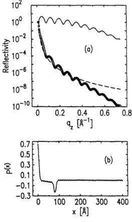
The first simulated profile, depicted as a solid curve in Fig. 1(a), resembles that of a thin film on a substrate. The corresponding reflectivity data of this profile appear in Fig. 1(b). With an aim to derive a correlation function P(x), we apply GTM to only two data points near the critical qz for total external reflectivity to determine the bulk density ½1. Then it is easy to obtain the
Fresnel reflectivity of the bulk density, shown as a dashed curve in Fig. 2(a), and R(qz)=RF(qz),
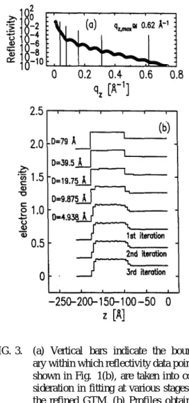
shown as a solid curve in Fig. 2(a). Employing Eq. (21), we obtain correlation function P(x) shown in Fig. 2(b). Because P(x) is the convolution integral of the derivative of the pertinent profile of electronic density, the inversive peak of function P(x) at 79Å reveals that the distance between two sharp edges of the profile along the perpendicular direction is about 79Å. Therefore, instead of being divided into layers arbitrarily but inflexibly in the original GTM [15] , the surface region of the sample is divided into layers of thickness D = 79, 39.5, 19.75, 9.875, 4.938 Å, respectively at separate stages of the refined GTM. At various stages the data points distributed within qz;m ax = ¼=D are taken into consideration for fitting [13]. The vertical bars, shown in
FIG. 1. (a) An original profile of electronic den-sity, and (b) reflectivity data for this pro-file.
FIG. 2. (a) Reflectivity data (circles) shown in Fig.1(b)with Fresnel reflectivityRF(qz)
(dashed curve) and R(qz)=RF(qz)
(solid curve). (b) Function P(x) obtained through Fourier transformation.
Fig. 3(a), indicate the boundary at which qz;m ax = ¼=D for values of D. The evolution of
profiles retrieved at consecutive stages of the GTM is illustrated in Fig. 3(b). If layers of thickness D = 4:938 Å are further divided into thinner layers of thickness D¼ 2:5 Å, data points distributed within qz;m ax = 1:2 Å¡ 1 are needed for reasonable fitting, but such data points in this case are
distributed only within the cutoff qz ¼ 0:74 Å¡ 1. In the final stage of the refined GTM only
data points within qz;m ax = 0:62 Å¡ 1 are thus fitted to construct the resultant GTM profile
with resolution D about 4.938 Å. In order to minimize the cost function between simulated and fitted reflectivity data, the whole GTM procedure, including all the stages, is undertaken in three iterations. A step-like profile, denoted “third iteration” in Fig. 3(b), is eventually obtained on fitting data within qz;m ax = 0:62 Å¡ 1. This step-like profile is successively smoothed. While
the SGTM is applied to the smoothed profile, the smoothed profile is re-divided into layers of thickness 4.245 Å. A relation between the thickness of divided layers and the boundary qz;m ax
of data considered for fitting is satisfied, i.e., 0.74 Å¡ 1 = ¼ =4:245 Å, and all simulated (or experimental) data within a cutoff qz = 0:74 Å¡ 1 are fitted to obtain the best resolution of
the retrieved profile. The computed reflectivity from the resultant SGTM profile is compared with simulated reflectivity data in Fig. 4(b). Satisfactory agreement is demonstrated between the simulated reflectivity data and the the computed reflectivity. Furthermore, the resultant SGTM profile and the original profile, shown in Fig. 4(a), are so similar that the dashed curve is scarcely distinguishable from the solid curve.
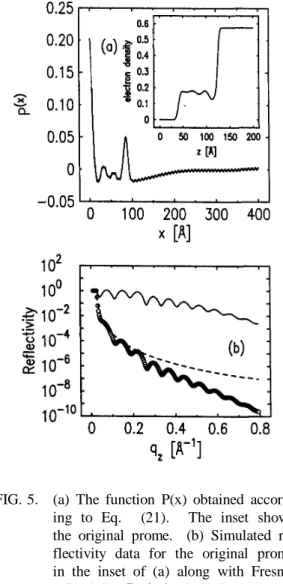
Another simulated profile, shown in an inset of Fig. 5(a), is inspired by x ray measurements on films of liquid hexane adsorbed on a rough silicon wafer [20]. The corresponding reflectivity R(qz) of this profile, the Fresnel reflectivity RF(qz) and R(qz)=RF(qz) are shown in Fig. 5(b).
According to Eq. (21), we obtain correlation function P(x) shown in Fig. 5(a). A large maximum of P(x) located at 84 Å indicates that the distance between two sharp edges of the profile in this example is about 84 Å. Using the refined GTM procedure, we divide the surface region into layers of thickness D = 84, 42, 21, 10.5 and 5.3 Å respectively at various stages. The qz;m ax , within
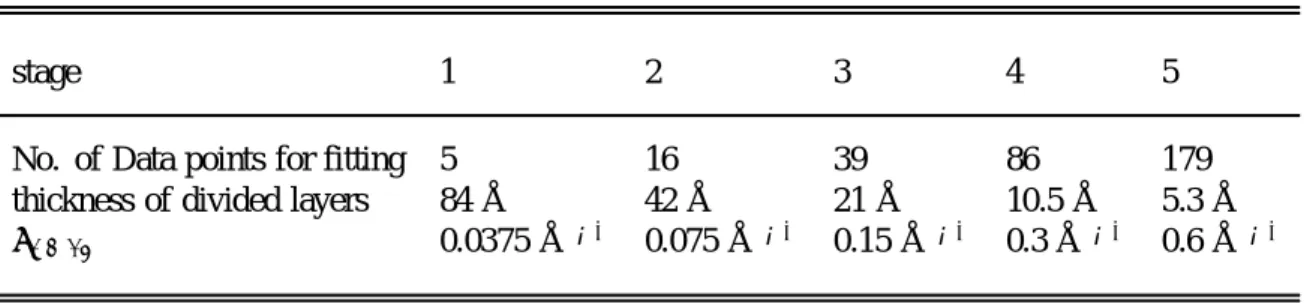
which data points are used for fitting, is determined as ¼=D for each value of D at each stage of the refined GTM and is indicated with vertical bars in Fig. 6(a). Related details of the GTM procedure are shown in Table I. The evolution of profiles, which are retrieved at successive stages
TABLE I. Data points for fitting at each stage in GTM.
stage 1 2 3 4 5
No. of Data points for fitting 5 16 39 86 179
thickness of divided layers 84 Å 42 Å 21 Å 10.5 Å 5.3 Å
FIG. 3. (a) Vertical bars indicate the bound-ary within which reflectivity data points, shown in Fig. 1(b), are taken into con-sideration in fitting at various stages of the refined GTM. (b) Profiles obtained at various stages of GTM with thickness of divided layers D = 79 Å, 39.5 Å,
19.75 Å 9.875 Å, and 4.938 Å, WIth profiles obtained after the first, second iteration and third iterations of GTM.
FIG. 4. (a) The resultant profile (dashed curve), retrieved from SGTM, compared with the original profile (solid curve). (b) Reflectivity data, shown in Fig. 1(b), compared with fitted reflectivity of the resultant SGTM profile in (a).
of the GTM and refined on operating the following GTM iteration, is illustrated in Fig. 6(b). In this case, we iterate the GTM procedure ten times to minimize the cost function between simulated and fitted reflectivity data. The resultant profile, denoted as “tenth iteration” in Fig. 6(b), is constructed, and, still being step-like, is smoothed. The SGTM is used to retrieve the resultant profile, shown in Fig. 7(a), while the smoothed profile is re-divided into layers of thickness ¼=(0:79 Å¡ 1).
FIG. 5. (a) The function P(x) obtained accord-ing to Eq. (21). The inset shows the original prome. (b) Simulated re-flectivity data for the original prome in the inset of (a) along with Fresnel reflectivity RF(qz) (dashed curve) and
R(qz)=RF(qz) (solid curve).
FIG. 6. (a) Vertical bars indicate a boundary within which data points are taken into consideration for fitting at various stages of GTM. (b) Profiles of electronic den-sity, obtained at various stages of the GTM, with thickness of divided lay-ers in a range 84 -5.3 Å. The pro-file obtained after GTM is iterated ten times, denoted as ”tenth iteration”, and the smoothed profile. ”CS” refers to a smoothing operation based on cubic-spline interpolation.
The retrieved profile reveals faithfully all features of the wetting-film region, whereas these are generally unknown in realistic cases. The reflectivity is fitted satisfactorily. Because we do not generate enough data points near the critical qz to define precisely the critical value of qz,
the bulk density, related to this critical value, can not be determined precisely and differs slightly from that of the original profile. The minute discrepancy arises as there is a small bump in the retrieved profile appearing at -80 Å (see Fig. 7(a)). For this reason minor deviations of fitted
FIG. 7. (a) The resultant profile (dashed curve), obtained from SGTM, compared with the original profile (solid curve). (b) Simulated reflectivity data compared with fitted reflectivity of the resultant SGTM profile in (a).
reflectivity spectra from simulated data are discernible beyondqz¼ 0:7 Å¡ 1in Fig. 7(b). In an experiment,
if good data near the criticalqzcan be obtained, the density of data points in this region becomes sufficiently
increased to determine precisely the accurate value of the critical qz and then to determine precisely the
value of the bulk density. In cases in which data near the criticalqz are poor, the bulk (substrate) density
should be determined in advance. The electron density of a substrate is generally known before preparation of the wetting samples.
IV. Conclusion
A new scheme for smoothed groove tracking is applicable to reflectivity data for samples for which profiles of electronic density are not completely smooth, whereas previous methods serve for reconstruction of only smooth profiles; in this way applications of SGTM are expanded. This scheme consists of a preliminary process, based on Fourier transformation, a refined GTM and the SGTM. In outline of the method, the surface region of the sample in question is divided into layers according to information on positions of sharp edges of the probed profile, which is obtained from the preliminary process. Then a refined GTM is used to retrieve efficiently the step-Iike profile of electronic density revealing basic features of sharp edges of the probed profile. Finally the SGTM is employed to reconstruct the resultant profile resembling the true profile and exhibiting details of minute features of the profile. The SGTM complemented with the preliminary process is applicable to simulated reflectivity data of samples as a thin film or a wetting film with little or no prior information.
A relation between thicknessD of divided layers and qz;m ax over which data points are taken into
consideration for fitting is qz;m ax = ¼=D. This rule must be rigorously satisfied whether in the refined
GTM with the preliminary process or in the SGTM. To violate the rule might cause a serious problem of a local minimum or make fitting futile.
In realistic cases measurement of reflectivity data near the critical qz, at which total external
re-flectance occurs, can be difficult, so that it becomes impossible to determine the bulk density based on experimental data, but the electronic density of a bulk or substrate is typically well known. Any accessory information, which is necessary and reliable for preparation of a sample or is provided by related theoretical work, is helpful in implementing efficiently the new scheme and in avoiding non-uniqueness of results. In this work using the new scheme with the refined GTM, we obtain quickly a step-like profile that resembles the real profile and serves as an estimated profile for the successive SGTM. A profile for the probed sample obtained by any other method dependent or independent of a model can serve as that estimated profile for the SGTM. During the iterative procedure of the SGTM, an estimated profile becomes further refined to approach the real profile in question as the computed reflectivity agrees satisfactorily with experimental or simulated data.
Acknowledgments
I thank Professors P. S. Pershan and X.-L. Zhou for insightful discussion, and the National Science Council of the Republic of China on Taiwan for support under grant No. NSC 88-2112-M-002-006. References
[ 1 ] S. Dietrich and A. Haase, Phys. Reports 260, 1 (1995).
[ 2 ] Proceedings of the 15th international conference on surface xray and neutron scattering, Physica B248 (1998).
[ 3 ] P. Mikulik and T. Baumbach, Phys. Rev. B59, 7632 (1999). [ 4 ] R. Lipperheide, et al., Physica B221, 514 (1996).
[ 5 ] N. F. Berk and C. F. Majkrzak, Phys. Rev. B51, 11296 (1995). [ 6 ] G. Reiss and R. Lipperheide, Phys. Rev. B53, 8157 (1996). [ 7 ] P. S. Pershan, Phys. Rev. E50, 2369 (1994).
[ 8 ] V.-O. De Haan, et al., Physica B221, 524 (1996). [ 9 ] V.-O. De Haan, et al., Phys. Rev. B52, 10831 (1995).
[10] M. V. Klibanov and P. E. Sacks, J. Math. Phys. 33, 3813 (1992). [11] W. J. Clinton, Phys. Rev. B48, 1 (1993).
[12] D. S. Sivia, W. A. Hamilton and G. S. Smith, Physica B173, 121 (1991). [13] C. H. Chou, Physica B233, 130 (1997).
[14] X.-L. Zhou and S. H. Chen, Phys. Rev. E147, 121 (1993).
[15] X.-L. Zhou and S. H. Chen, Phys. Reports 257, p. 310-322 (1995). [16] X.-L. Zhou and S. H. Chen, Phys. Rev. E47, 3174 (1993).
[17] C. H. Chou, et al., Phys. Rev. E55, 7212 (1997).
[18] C. H. Chou, Solid State Comm., Vol 108, No. 9, 687 (1998). [19] G. Parratt, Phys Rev. 95, 359 (1954).