Performance modeling and analysis of load balancing policies with priority queueing

(1)

J. SYSTEMS SOFTWARE 169 1993; 20:169-187

Performance

Modeling and Analysis of Load

Balancing Policies with Priority Queueing

Rong-Chau Liu

Chung Shan Institute of Science and Technology, Lungtan, Taiwan, R.O.C.

Sheng-De Wang

Department of Electrical Engineering, National Taiwan University, Taipei, Taiwan, R.O.C.

In this article, we study an adaptive load-balancing algorithm in the homogeneous distributed systems in

which only local status information is used. The pa-

rameters affecting the performance of the load-bal-

ancing algorithm are investigated. Jo analyze the ef- fects of service disciplines on load balancing, we study two classes of service disciplines, impartial discipline and partial discipline. In impartial discipline, all tasks

in the system are treated alike. Partial disciplines

divide tasks into two classes, local tasks and remote tasks, and then assign different priorities to them. Five

partial disciplines with different priority assignment

rules are compared. The numerical results are pre-

sented and used to shed light on the characteristics of

the load-balancing process.

1. INTRODUCTION

Distributed computer systems have many advan-

tages, including the capability to share processing of

tasks in the event of overloads and failures, trans- parency, and modulari~. In a distributed system a task might wait for service at the queue of one server while at the same time another server capable of serving the task is idle. This phenomenon was clearly demonstrated by Livny and Melman [l], who showed that in a network of homogeneous, au- tonomous nodes, there is a high probabili~ that at least one node is idle while tasks are queueing at some other node or nodes over a wide range of

Address correspondence to Professor Rong-Chau Liu, Chung Shun I~titu#e of Science and Tech~~o~, P.O. Box ~8-9-3, Lungtan, Taiwan, R. 0. C.

network size and node utilizations. A load-balancing policy designed to minimize the mean turnaround time of the task will tend to prevent the system from reaching such a state. System performance can be improved by transferring workload from heavily to lightly loaded nodes.

Load-balancing policies may be either static or adaptive. Static policies only use information about the average behavior of the system; transfer decisions are independent of the actual current system state. Numerous static load-balancing policies have been proposed. Stone [2, 31 and Bokhari [4] exam- ined the deterministic algorithms of task assign- ments. Tantawi and Towsley [51 developed a technique to find optimal probabilistic assignment rules. The principal advantage of static policies is their simplicity: there is no need to acquire and maintain information on the system state. By contrast, adaptive policies are more complex, since they use information of the current system state in making transfer decisions. Several adaptive load-sharing policies have been reported. Two strategies for adaptive load sharing with distributed control were investigated by Eager, Lazowska, and Zahotjan [6]. Wang and Mor- ris [7] compared a number of server- and source-ini- tiative adaptive algorithms.

The motivation behind this article is to investigate the effects of processor service disciplines on load- balancing policy, which have not been discussed in the reports mentioned above. First, we study a simple adaptive load-balancing policy and analyze the effects of its parameters on system performance. Owing to different service disciplines, tasks in the

0 Elsevier Science Publishing Co., Inc.

(2)

170 J. SYSTEMS SOFIWARE 1993; 20:169-187

system are divided into two classes: local tasks, which are processed at their site of origination, and remote tasks, which are processed at some other sites in the system after being transferred through an interconnection network. We also examine the effects of assigning different priorities to two classes of tasks. Five such policies are developed, ranging from one favoring local tasks to one favoring remote tasks. Analytic queueing model and simulation results are used to study the interdependence between the system parameters and the behavior of these load-balancing policies.

The remainder of this article is organized as follows. In section 2, we briefly describe the system architecture. Section 3 comprises the description of load-balancing policies and the mathematical analysis of the decomposition approximation model. In section 4, we describe the numerical and simulation results of this research. Section 5 concludes the article.

2. SYSTEM MODEL AND ASSUMPTIONS

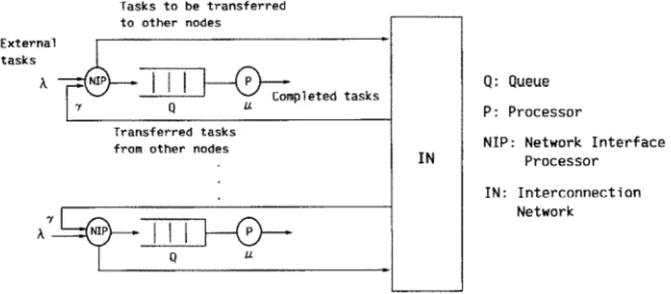
We present a distributed system as a collection of IV identical nodes. The nodes are connected by an interconnection network (IN). The system architecture is shown in Figure 1. Each node in the system consists of a processor, a network interface processor (NIP), and a queue. The NIP performs the load-balancing algorithm and is responsible for com- municating with the interconnection network. Tasks entering the node from the external world (AI or from the interconnection network (y) are selected by the NIP, based on a specific load-balancing policy. Then the accepted tasks enter the queue and wait for the service of the processor; the remaining tasks are transferred to the interconnection network.

Tasks to be transferred to other nodes

R.-C. Liu and S.-D. Wang

There are several assumptions to simplify the system model, which are stated as follows.

Homogeneity. The nodes are identical and are

subject to external task arrival Poisson processes with the same rate A; the service time of the processor is exponentially distributed with mean l/p.

FFhen a task is tra~fe~ed to the interconnection network for remote processing, the task incurs a com-

munication delay. This delay includes the communi-

cation cost, which is a cost between the NIP and the interconnection network and includes packing data, transmitting data, receiving data, unpacking data, and the transmission delay in the interconnection network. We lump these effects together as communication overhead (Cob), which is incurred by the load-balancing algorithms when a task is transferred to the other nodes through the IN. We also model the communication channel as a single-server queueing system whose service time is an exponentially distributed random variable with mean l/pi”.

The processing cost of NIP is much smaller than that

of the processor. That is, the load-balancing algo-

rithm performed by the NIP does not interfere with the processor; therefore, the processing cost of the NIP is ignored.

~ecomposa~i~i~. We assume, in the steady state,

that the task arrivals from the interconnection network are of Poisson type and the interarrival time of the transferred task is an exponentially distributed random variable with mean l/y. Based on this decomposition approximation, we can decompose the system model so that the model for each node can be independently analyzed.

External I I I

(3)

Load Balancing with Priority Queueing

3. LOAD-BALANCING POLICIES AND QUEUEING ANALYSIS

3.1 Load-Balancing Algorithm

A distributed load-balancing algorithm is composed of two main elements, the probing element and the decision element. The decision element determines when, from where, and to whom to transfer a waiting task. The decision is made according to the current available information on the state of the system. The probing element collects this status information for the decision element. We consider here a simple and straightforward algorithm. The probing element only collects the local status (queue length) of the node, and the decision element accepts rejects an arriving task, depending on this local status information and a predefined threshold Clh) value. The algorithm is as follows: when an arriving task enters the node, if the NIP finds the local queue length, including tasks waiting in the queue and the task in service, is Th, then this task is transferred through the interconnection network to a randomly selected node in the system with equal probability. Otherwise, this task is accepted and goes into the queue.

This algorithm can cause instability. That is, in a heavily loaded network, when all nodes in the system have a queue length larger than the Th, the system will enter a state in which the task arrivals are always transferred back and forth within the network and no processor accepts them. This instability phenomenon can be overcome by adding an appropriate control policy to the decision element. The simple control policy we adopt here is to restrict the number of times that a task can be transferred to a predefined transfer limit (Tl) value [8]. Then the load balancing algorithm is updated as follows.

When an arriving task enters the node, if the NIP finds the local queue length of the node is lower than the Th or the number of times that the task has been transferred and a message carried by the task is equal to the Tl, then this task is accepted. Other- wise, the transfer count of the task is increased by one and the task is transferred to a randomly selected node in the system. The initial value of the transfer count of a task from the external world is

set at 0.

3.2 Service Disciplines

Another question that arises in havior of the refined algorithm

considering the be- is how the destina-

J. SYSTEMS SOFTWARE 171 1993; 20:169-187

tion node should treat an accepting transferred task from the interconnection network: tasks may be given different service attributes in the local site or in the remote site. We consider two classes of service disciplines and describe them in the following discussion.

3.2.1 Impartial discipline. In this discipline, the destination node treats an arriving transferred task as a task originating at that node. Then all accepted tasks, assigned with the same priority, enter the queue and follow the first come, first-served scheme to wait for the service of the processor. We call this an Fl discipline.

3.2.2 Partial disciplines. In these disciplines, owing to the different service attributes, tasks are divided into two classes-local tasks, referring to tasks processed at their own site, and remote tasks, which processed at some other site in the system after being transferred through the interconnection network. Local tasks come either from the external world directly or from the interconnection network. Tasks transferred to another node because of the limitation of the local task Th are later transferred back to the same node because of the effect of the Tl. Since the system has two classes of tasks, we define LQ and RQ, respectively, as random variables denoting the number of local tasks and the number of remote tasks at a node; Th, and Th, are the values of the threshold of the local task and remote task, respectively. Two types of partial disciplines use different priority assignment schemes as defined below.

1. Priority Queueing [9] Disciplines a. Local tasks first (LTF) policy

i.

ii.

If an arriving task from the external world finds the local task queue length of the node is Th,, then the transfer count of the task is incremented by one and the task is transferred to a randomly selected node in the system with equal probability. Other- wise, it is processed locally.

Arriving tasks from the interconnection network can be divided into two cases. Local tasks: if the transfer count is Tl, then this task is accepted. Otherwise, its transfer count is increased by one and it is transferred to a randomly selected node. Re- mote tasks: if the remote task queue length of the node is lower than Th, or the trans-

(4)

172

. . . 111.

J. SYSTEMS SOFTWARE 1993; 20:169-187

fer count is Tl, then this task is accepted for processing locally. Otherwise, its transfer count is increased by one and it is transferred to a randomly selected node. Tasks at each node are processed according to a priority discipline with nonpreemp- tion allowed. Tasks having the same priority are processed in a first come, first served manner.

iv. Local tasks are given higher priority than remote tasks.

b. Remote tasks first (RTF) policy i. Same as LTF policy. ii. Same as LTF policy. iii. Same as LTF policy.

iv. Remote tasks are given higher priority than local tasks.

c. Long queue first (LQF) policy i. Same as LTF policy. ii. Same as LTF policy. iii. Same as LTF policy.

iv. Local tasks are given higher priority than remote tasks when LQ 2 RQ. Otherwise, remote tasks are given higher priority than local tasks.

d. Short queue first (SQF) policy i. Same as LTF policy. ii. Same as LTF policy. iii. Same as LTF policy.

iv. Local tasks are given higher priority than remote tasks when LQ I RQ and LQ > 0. Otherwise, remote tasks are given higher priority than local tasks.

2. First come, first served (F2) policy i. Same as LTF policy. ii. Same as LTF policy.

iii. Tasks at each node are assigned with the same priority and follow the first come, first served scheme to wait for the service of the processor.

3.3 Queueing Analysis

Based on the decomposition approximation mentioned above, we can simplify the queueing analysis by assuming that the state of each node is stochasti- tally independent of that of any other node. Each

node can then be analyzed in isolation. The effect of the remainder of the system on an individual node is represented by an arrival process of transferred tasks from the interconnection network. Because the network is homogeneous, system performance measures can be obtained by analyzing a model of any individual node. We will discuss the accuracy of this decomposition approximation at the end of section 4.

Owing to the complexity, the mathematical analysis is only tractable for cases when Tl = 1. The independent analysis of each individual policy will be described in the following subsections.

3.3.1 Tl = 1: Impartial discipline (Fl). In this case, p (the probability that the portion of transferred

tasks have their transfer count equal to Tl) = 1. Let E[Q] be the mean queue length of the node. We can show that

E[QI =

i [

(P+

Pl)

l-(P+PJTh

(1 -

P -

Pd2

lwP +

PdTh

-

1-P-R

₁ where A Y P= i,P, = -,and PO P [

l-b+dTh

+ (P+PJTh

-1

=

1-P-h

l-P,

₁

.

Let E[T] be the mean task response time. From Little’s formula [lo] and the fundamental queueing theory [ll], we have

E[T] = h

E[Ql

+ ;E[Coh], 1

where E[Coh] = denotes the mean com-

Pin - NY

munication overhead. The y (mean transferred task

(5)

Load Balancing with Priority Queueing J. SYSTEMS SOFTWARE 173 1993; Z&169-187

arrival/departure rate) is a function of h, Th, and Tl, which can be calculated by a recursive substitution technique (see Appendix A).

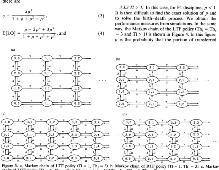
3.3.2 Tl = 1: Partial disciplines. In this case, the remote task threshold, Th,, has no effect on the load-balancing policy. As the decomposition approximation stated above, each node in the system under load-balancing policies can be represented by a con- tinuous time and discrete state Markov chain. Fig- ure 3 shows the state transition diagrams for a node executing four priority queueing disciplines, ,respectively, when Th, = 3 and Tl = 1. The state (I, r) denotes that there are f local tasks and r remote tasks in the node, respectively, and P(1, r) is the probability that the node is in the state (I, r).

Let E[LQ] and E[RQ] be the mean number of local tasks and mean number of remote tasks in the node, respectively. For the LTF policy, we can find the closed-form expression for y, E[LQ], and E[RQ]. Using the 2 transfo~ technique (see Appendix B), there are hP3 Y= 1 f p + p2 + p3 ’ E[LQ] = p + 2p* + 3p3 1 + p + p* + p3 ’ and (3)

(4)

(4 . . .

EiRQl

pl( p6 + 3p5 + 6p4 + lop3 + 6p2 f 3p + 1) = (1 + p + p2 f p3)[1 - pl(l + p + p* + p”)] . (5)

The other three priority queueing disciplines can be analyzed by the matrix-geometric solution technique [121. This technique has been used in the performance modeling and analysis of the nonprod- uct form queueing networks [131, which yield exact solutions of E[LQ] and E[RQ] for each node (see Appendix C). Thus, the mean task turnaround time

03TI) is

E[T] =

JWQI +

J-WQI +

~ELCohl

A _p ’ (6)

where E[Coh] is the same as in Equation 2. As mentioned above, the value of y can be calculated by a recursive substitution technique.

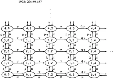
3.3.3 TI > 1. In this case, for Fl discipline, p < 1. It is then difficult to find the exact solution of p and to solve the birth-death process. We obtain the performance measures from simulations. In the same way, the Markov chain of the LTF policy (Th, = Th, = 3 and Tl > 1) is shown in Figure 4. In this figure, p is the probability that the portion of transferred

Figure 3. a, Markov chain of LTF policy (Tl = 1, Th, = 3). b, Markov chain of RTF policy (Tl = 1, Th, = 3). C, Markov chain of LQF policy (T1 = 1, Th, = 3). d, Markov chain of SQF policy (Tl = 1, ThB = 3).

(6)

174 J. SYSTEMS SOFTWARE

1993; 20:169-187 R.-C. Liu and S.-D. Wang

Figure 4. Markov chain of LTF policy (Tl > 1, Th, = 3).

. . .

local tasks have their transfer count equal to Tl and q is the probability that the portion of transferred remote tasks have their transfer count equal to Tl. We note that p + q < 1. The exact solution of this Markov chain is too complicated to be obtained by mathematical methods. Thus, we again obtain the performance measures from simulations for partial priority queueing disciplines.

3.3.4 F.2 ~scipli~e. Even when the decomposition appro~mation is valid and Tl = 1, the analytic analysis for the F2 discipline is not tractable. Thus, we obtain the performance measures of this discipline from simulations.

4. RESULTS

In this section, we present the performance measures of the load-balancing policies stated in section 3. As mentioned above, some situations, such as Tl > 1, are too complicated to analyze using the mathematical methods, simulation is the most popu- lar approach for the analysis of the performance of a computer system because of its generality and simplicity. Therefore, we use results from simulations to depict the actual sample means. At the end of this section, we will discuss the relationship between simulation results and those of the mathematical analysis.

The simulation model is constructed on a SUN/4 workstation using PAWS (performance analyst’s workbench system) simulation language [14]. Over 100 cases have been simulated. The lengths of the simulation runs are determined over a considerable range of parameter values by a suitable compromise between numerical accuracy and the completion time for simulations. All results have confidence intervals [15] of I 5% a 90% confidence level. The key

performance metric of these experiments is the mean turnaround time of tasks (Rt). Furthermore, in the following experiments, we let the mean task service time, l/l.~, equal one unit; all measurements of the turnaround time are in terms of this unit.

Since many parameters, such as the system load ( p), threshold (Th), transfer limit (Tl), communication overhead (Cob), etc., can affect the performance of load-balancing policies, we adopted a “one factor at a time” approach in our simulation experiments; that is, each experiment involves the varying of one parameter while keeping the others at a constant value. The variable parameter in each experiment is represented by the abscissa of the corre- sponding result graph, whereas the values of the fixed factors are included in the figure legend. The number of nodes in the system (N) is fixed at 10 in all simulation runs. In general, although it is possi- ble for the communication overhead of the interconnection network to be > 10% of the mean task service time, it would not occur frequently. Hence, we assume the communication overhead is 5% of the mean task service time, i.e., I*in = 20, unless otherwise mentioned.

In the following experiments, we first investigate the effects of system parameters on the performance of impartial discipline (Fl), and then compare the performance of Fl discipline with those of partial disciplines.

4.1 Fl Discipline

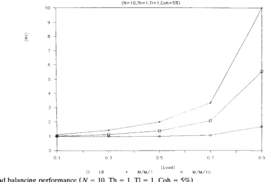
4.1.1 Perfbmance compa~so~. The prelimina~ perfo~ance measures of the load-balancing algorithm are shown in Figure 5. The results are compared with two bounds, represented by the M/M/l model (no load balancing) and the M/M/N [ill

(7)

Load Balancing with Priority Queueing J. SYSTEMS SOFTWARE 175 1993; 20:169-187 10 (N=IO.Th=l,TI=1.Coh=5%) 0-m I , 0 I 03 05 0 7 (LO&) M/M/l 0

Figure 5. Load balancing performance (NC = ;;I, Th =‘I, Ty’!‘;, Coh = 05%).

I -4

“9

model (perfect load balancing with no costs). From this comparison, we find that even an extremely simple load-balancing algorithm can achieve sub- stantial performance improvement over no load balancing. The improvement is much more pronounced as the load increases. For instance, at p = 0.9, the turnaround time of the load balancing is about 5.5 units, whereas the M/M/l turnaround time is 10 units, a significant difference. It is clear that the algorithm performs worse than the exact M/M/10 model. For instance, at p = 0.9, M/M/10 results in a turnaround time of about 1.6 units. 5

To clearly present how much performance improvement (PI) can be achieved by the load-balancing policy, we define the PI factor as follows:

PI(%) = (T”lb -

T,b)/T”,b

x

loo%,

where T,, CT”,,,) is the mean task turnaround time of the node with (without) load balancing. At extreme load condition, p = 0.9, the PI value is 44.3%. The performance of the load-balancing policy can achieve much more improvement because of the variation of system parameters, which will be described in the following subsections.

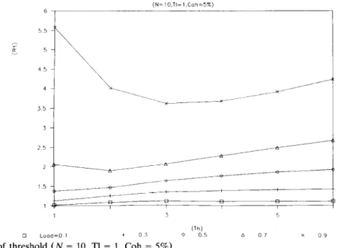
4.1.2 Effect of Th. Threshold is a fundamental parameter of the load-balancing policy. It determines when a task transfer will be attempted. Intu- itively, a low Th is appropriate at low system loads because the probbility is high for a transferred task to “find” a node where the queue length is lower

than the Th. However, at high system loads, a high Th is appropriate because in these conditions, most nodes have high queue length. However, high Th will reduce the task transfers and hence reduce the effects of load balancing, so the Th should be selected carefully.

Figure 6 shows the phenomenon stated above. The optimal Th is 1 for low and medium system loads ( p I OS), 2 for high system loads ( p = 0.71, and 3 for extreme high loads ( p = 0.9). Based on this attribute, in the following experiments we use the adaptive threshold (A = Th) policy (i.e., Th = 1 for p 5 0.5, Th = 2 for p = 0.7, and Th = 3 for p = 0.9) for simulations.

Another parameter affecting the value of optimal Th is the Coh. It is clear that low Th are appropriate for low Coh; high overheads demands higher Th.

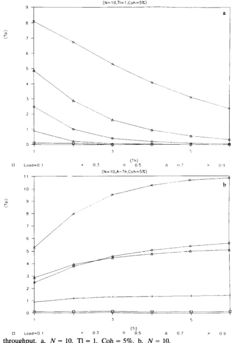
4.1.3 Effect of TZ. With a Tl, tasks are allowed to be transferred multiple times in searching for a suitable node. Thus, the probability of a successful transfer at Tl > 1 is higher than at Tl = 1; system performance will also be improved.

Figure 7 shows mean turnaround time versus Tl for different system loads. From this figure, we observe that the higher the value of the Tl, the better the system performance will be. However, this improvement will be saturated when the value of the Tl is larger than a specific value. This phenomenon occurs because the performance improvement caused by the high probability of successful task

(8)

176 J. SYSTEMS SOFTWARE 1993; 20:169-187

z- a 55 5 45 15 I 3 5 (Th) Load=0 thrisholcl (N 1 1,‘Coho 1 0 05 a 07 x “9 Figure 6. Effects of = 10, Tl = 5%).

transfer will be offset by the Coh under high-T1 conditions. From our simulation experiments, the specific Tl is about 3 for p < 0.5, about 4 for 0.5 5 p

I 0.7, and about 5 for p > 0.7. As for Th, the Coh will also affect the selection of Tl. Clearly, at high Coh low Tl is appropriate; high Tl are for systems with lower overheads.

Based on these observations, we can make opti-

ma1 choices for different conditions. For instance, at p = 0.9, Th = 3, and Tl = 5, the PI factor is 70.3%, which is a significant improvement over no load balancing.

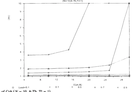
4.1.4 Effect of Coh. As mentioned above, cases where the Coh of the interconnection network is

> 10% of the mean task service time do not occur

(N=1O.A-Th,Coh=S%)

38

18

---a--___

16

(9)

frequently. However, we investigate the effect of this parameter just for theoretic analysis. Figure 8 shows the mean task turnaround time versus Coh for different system loads. In this figure, the results of p = 0.5 at Coh = 30% and p = 0.9 at Coh 2 20% are beyond the scale of the graph. For p d 0.3, the Coh has almost no effect on system performance. However, the system turnaround time increases dra- matically at high overheads. This phenomenon proves that the queueing delay in the communication channel is a predominant factor in the mean task turnaround time at high overheads.

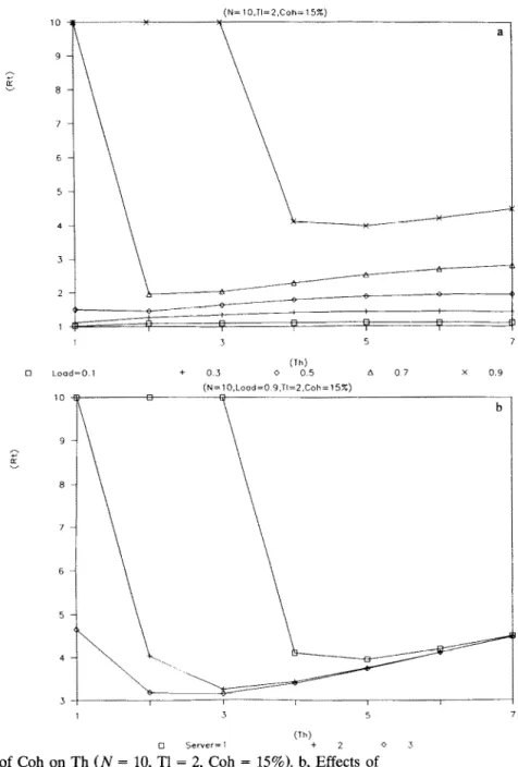
An interesting phenomenon occurs at Coh = 30%, where the turnaround time of p = 0.7 is lower than that of p = 0.5. This is due to the A-Th policy (i.e., Th = 1 for p = 0.5 and Th = 2 for p = 0.7) that we applied in simulations. Thus, we can imagine that these Th are not the optimal values at high overhead conditions, The description related to the effect of Coh on Th in section 4.1.2 is verified again. This phenomenon will be clearer in the following experiments. Figure 9a (some results are beyond the scale of the graph) shows the effect of Coh on the selection of optimal Th. We can observe that under Tl = 2 and Coh = 15% environments, the optimal Th at p = 0.5 is 2 instead of 1 and at p = 0.9 is 5 instead of 3. Figure 9b shows the effect of the network server on system pe~o~ance. We focus experiments on extreme high load C p = 0.9) conditions. We observe that enhancing the capability of the communication channel will significantly improve system performance for high-load and low-Th

J. SYSTEMS SOFTWARE 177 1993; Z&169-187

environments. However, this improvement is not so clear in high-Th environments. These observations provide some tradeoffs in the design alternatives of the interconnection network.

4.1.5 before t~ruug~p~t. In this section, we consider the network traffic, N x y, resulting from task transfers. It is clear that network throughput increases (decreases) with an increase in Tl (Th). Figure 10a shows the network throughput versus system load for different Th. We observe that the higher the Th the lower the network throughput will be. The network throughput versus Tl for different system loads is shown in Figure lob. We observe that when the system load is < 0.5, the network traffic is small; therefore, it is easier to approach saturation. This is due to the fact that, at low system loads, there is a high probability of successful task transfer. However, when the system load is > 0.5, the network traffic increases substantially and approaches saturation at high Tl. For instance, at p = 0.9, the network traffic will approach saturation when Tl > 10 and the throughput is about 17 (not shown in Figure lob). Another interesting phenomenon is that the network throughput at p = 0.7 is smaller than at p = 0.5, when Tl > 3. This is due to the effect of the A-Th policy 0-h = 1 at

p = 0.5 and Th = 2 at p = 0.71 that we applied to

simulations.

Intuitively, the greater the activity of load baianc- ing, the heavier the network traffic will be. Thus, one may imagine that the larger the network

(N=IO,A-Th,TI=I) ‘*

1v

-. ---

K

I / P. n’ 9 -- 8- 7- 4 8 12 I6 20 ‘!a LS (COh.%) Coh”cN Load=O. 1 1;. 03 0 0.5 a O? x OY

(10)

178 J. SYSTEMS SOFTWARE 1993; 20:169-187

(N= 10,11=2,Coh=15%) 10 a 9 7 6 Oh) L7 iood=O., + 03 0 0.5 A 07 x 3.9 i 3 5 7 WI Server=l 2

Figure 9. a, Effects of Coh on Th (N = 10, ;1 = 2, Coh = 15%). b,‘Effects of0 3 nehvork server (N = 10, Load = 0.9, Tl = 2, Coh = 1.5%).

throughput, the higher the PI will be. However, this is valid for environments with fixed Th and Coh. This phenomenon is verified by comparing Figures 10b and 7. When Th is a variant factor, the above statement is no longer true, as can be seen by comparing Figures 10a and 6.

4.2 Partial Disciplines

We apply the A-Th policy stated above (Th, = Th, = 1 for p 5 0.5, Th, = Th, = 2 for p = 0.7, and Th, = Th, = 3 for p = 0.9) to the following experiments.

The network throughput can be used to determine 4.2.1 P~~~~~nc~ comparison. Figure 1 la shows a the minimum network bandwidth (BW). For exam- comparison of the PI factor of the Fl discipline with ple, if the size of a task is K bits, the minimum BW those of five partial disciplines. In this figure, at is N x y x K. In other words, for a given network p = 0.95, the performance of the SQF policy is worse bandwidth, the network utihzation is (N X y X (PI < 0) than that of the condition in which no load

(11)

Load Balancing with Priority Queueing J. SYSTEMS SOFTWARE 179 1993: 20:169-187 (N=lO,TI=l,Coh=5%) ‘)->-a 1 3 i Oh) 0 Luod=O I + 0.7 c’ 05 A 0 7 x 0 ‘, (N=lO.A-Th,Coh=5%) 0 , / ,

4

1 3 5 01) Load=0 thr&$put. 1 T; 03 i%.‘i, I;, 07 x 09

Figure 10. Network a, N = 10, = 1, Coh = N =

A-TX, Coh = 5%.

mance of the Fl discipline is better than those of the partial disciplines. This is not hard to under- stand: under the Fl discipline, the transferred tasks from the interconnection network are treated alike, with tasks originating from the external world at that node. However, under the partial disciplines, if the local and remote tasks are assigned different priority levels for processing in the processor, then the queueing structure of the tasks in the node will be changed because of the transferred task arrivals. Intuitively, we can imagine that the disciplines favoring the remote tasks will result in shorter mean remote task turnaround time and longer mean local

task response time. However, in voring the local tasks, shorter

the disciplines fa- mean local task turnaround time and longer mean remote task turnaround time will be obtained. Let E[LT] and E[RT] be the mean local task turnaround time and the mean remote task turnaround time, respectively. When Tl = 1, the mean task turnaround time is

E[T] = hE[LT] A-Y + XE[RT],

₍₇₎

where E[LTl = E[LQl/(h - 7) and E[RT] = E[RQI/y + ElCohl. For small y, because E[T] = E[LTl and tasks in the system are almost all of

(12)

180 J. SYSTEMS SOFTWARE 1993; 20:169-187

(N= 1 O.A-Th.TI= 1 .Coh=5%) a 0 01 03 05 07 09 (Load) F2 + RTF 0 LTF A LOF x S”F v FI (N= 1 O,A-Th,TI=Z,Coh=5%) 80 70 5 a 60 50 40 30 20 10 0 , I I / I I 1 I I 01 03 05 07 0.9 (Load) LTF

Figure 11. Performance improvement. ayTFN = 10, l-Th, Tl = 1, “,oh”L 5%. IJ,~

SQF v Fl

N= 10, A-Th, Tl = 2, Coh = 5%.

“local” type, all partial disciplines will have almost SQF policy usually assigns higher priority to the the same performance. However, if the y is large, local tasks. A comparison of the performance im- the E[RT] becomes a dominant factor in the E[T]

and the performance of the disciplines favoring remote tasks will be better than those of the disciplines favoring local tasks.

The descriptions stated above can be verified in Figure lla. At low and medium system loads ( p I 0.5) and small y, disciplines have almost the same performance. However, at high system loads ( p 2 0.7) and large y, the RTF policy results in the best and the SQF policy results in the worst performance. This is due to the fact that, at high system loads, the

provement of different disciplines at Tl = 2 is shown in Figure llb. In the same way, the Fl discipline results in the best performance. However, in the partial disciplines, the RTF policy performs best, the LTF policy performs worst, and the LQF and F2 policies have almost the same performance over the entire range of the system loads.

4.2.2 Throughput comparison. Figure 12a shows the comparison of the network throughput of the Fl discipline with those of the partial disciplines. From

(13)

Load Balancing with Priority Queueing J. SYSTEMS SOFTWARE 181 1993; 20:169-187 (,,-_ io,A-Th.Tl=1.Coh=~%) (Loud) 0 F2 * RTF 0 LTF a LOF * WF v i 1 jN=,O,A-Th,Tt=Z.Coh-9%) 12 -r---- _ .__-I__ .-~ 01 0-T 05 07 05 (Good) LTF

Figure 12. Throughputfl~~~parison: a, “z = 10, ,kTh, Tl = 1, >oh’z 5%. blx

SQF D Fl

N = 10, A-Th, Tl = 2, Coh = 5%.

this figure, we can observe that the network throughput of the Fl discipline is always higher than those of the partial disciplines. At low and medium system loads ( p I OS), the partial disciplines have almost the same throughput. The larger the network throughput, the higher the probability of successful task transfers will be; the larger the throughput, the better the performance will be. This phenomenon can be observed in Figures lla and 12a. Exceptions are the SQF and the LTF policies at extreme high- load conditions. The throughput comparison at Tl = 2 is shown in Figure 12b. We find that the effect of

the Tl on the FI discipline is more pronounced than on the partial disciplines.

The reason why the SQF results in the worst performance at p r 0.9 and Tl = 1 can be described as follows: The SQF discipline assigns higher priority to the minority tasks in the system, which results in a large queueing delay for the majority tasks and significant performance deterioration. Thus, at extreme high-load conditions and Tl = 1, the performance of SQF is worse than that of LTF. This phenomenon is more pronounced at p = 0.95, in which SQF results in a turnaround time of about 50

(14)

182 J. SYSTEMS SOFTWARE 1993; 20~169-187

units and LTF results in a turnaround time of about 9.6 units. However, at large Tl, the effects of ioad balancing (large y) will improve the performance of SQF significantly, this leads to the situation in which the performance of SQF is slightly superior to LTF. 4.2.3 High threshold at extreme high-system-load co~d~t~o~~, As mentioned above, the SQF policy al- most results in the worst performance in the partial disciplines because it assigns higher priority to the minority tasks and results in a large queueing delay for the majority tasks. However, if the queue length

difference between the local and remote tasks is small (under high-Th environments), then the SQF policy will perform well because of the reduced turnaround time for minority tasks and the insignif- icant queueing delay for the majority tasks. This description is verified in Figure 13a. We focus the experiments on extreme high-load conditions ( p = 0.95). We observe that the SQF policy results in the best performance when Th 2 18. Because high Th are for systems with higher Coh, we can image that the SQF policy will perform well in high-overhead systems. Figure 13b shows this phenomenon. We

(N=10.~ood=0.95,11= ,.Coh=lj%)

a

(Th)

q F2 + ATF LOF x SOF

b 5

1

3 2 :,.~ 0 -y-VI-m---m’- 3 5 7 ‘) 1 I I’! I i 17 1’8 (Th)

Figure 13. Effects of high Thy a, G = 10, ‘,,a:‘= 0.95, ;I =‘;‘, Coh =*5%~~,

x WF N = 10, Load = 0.95, Tl = 2, Coh = 15%.

(15)

also observe that under high-overhead and low-Th (Th = 3) environments, the RTF policy results in the worst performance and the LTF policy has the best performance. Based on the observation mentioned above, we can conclude that for partial disciplines at low Coh the RTF policy is appropriate; the SQF policy is suitable for systems with higher overheads.

4.3 Accuracy of the Decomposition Approximation

The mathematical queueing analysis described in section 3 is valid under the assumption that all nodes in the system are stochastically independent. The effect of the remainder of the system on an individual node is represented by an arrival process of the transferred tasks from the other nodes in the system. We also assume that this is a Poisson process. These assumptions lead to a decomposition approximation model in which each node in the system can be analyzed in isolation. Here we investigate the accuracy of this approximation. Let Sim and Num be the results from simulations and numerical solutions of the analytic model, respectively. The deviation (S) is defined as a(%) = 1Sim - Num/SimI X 100%.

Figure 14 shows the deviations of the Fl, RTF, and LQF policies versus system load when N = 10 and N = 20, where FlO, RlO, and LlO depict the curves of Fl, RTF, and LQF with N = 10, respectively. From this figure we observe that there is a

14 13 12 10 J. SYSTEMS SOFTWARE 183 1993; 20:169-187

very good consistence; the deviation is < 2% be-

tween the analytic model and the simulation when p I 0.5. However, the higher the system load, the larger the deviation will be. At high system loads, for instance, at p = 0.9 and N = 10, the deviation is

> 13%. These errors came from the effects of the decomposition approximation and the assumption that the transferred task process is a Poisson process. However, these effects are reduced when N is large. For instance, at p = 0.9 and N = 20, the deviation is < 8%. Based on observations from various simulation experiences, this is because the larger the system size, the more the transferred task process (y) is similar to a Poisson process. This leads to a situation in which the approximation is reduced for large systems. Thus, we can conjecture that the approximation error of the analytic model will approach 0 when the system size, N, approaches infinity.

The analytic queueing analysis described in section 3 is limited to Tl = 1 cases. Based on our experiments, the execution time of the simulation under extreme high-load conditions with p = 0.9 and Tl = 1 on a SUN/4 machine with 16 MIPS capability using PAWS language more than two hours. However, the same experiment, following the mathematical approach, running on an IBM-PC (80386 + 80397) with 4 MIPS capability using MAT- LAB language obtains a result of about 10 seconds. This is a significant difference that can be easily observed. Thus, if the analytic approach can be extended to Tl > 1 cases, a pronounced benefit will

(&Th,TI=,.Coh=5%)

(16)

184 J. SYSTEMS SOFIWARE 1993; 20~169-187

be obtained. For Tl > 1 conditions, the Markov chain approaches infinity two dimensionally, as depicted in Figure 4, some parameters, p and 9, are too complicated to determine analytically. The mathematical analysis with further approximation might be a feasi- ble approach. This interesting research area requires further investigation.

5. CONCLUSIONS

This study was concerned with the performance analysis of a simple load-balancing algorithm with different service disciplines. The six disciplines we investigated were Fl, LTF, RTF, LQF, SQF, and F2. The analysis of the policies was carried out using two approaches, i.e., simulation and mathematical method.

The mathematical modeling of the Markov process of the entire system appeared to be computa- tionally intractable. Thus, we made some assumptions and applied a decomposition technique to solve the simplified Markov process using the Z transform and matrix-geometric solution techniques.

The policies were tested over a large range of parameter values. Some salient observations are as follows.

An extremely simple adaptive load-balancing algorithm that only collects local status information yields dramatic performance improvement over no load balancing.

The optimal Th of the policy, under a realistic value of Coh, is 1 for p 5 0.5, 2 for 0.5 < p < 0.9, and 3 for p 2 0.9.

The performance of the load-balancing algorithms is insensitive to the effect of the Tl at low and medium-sized system loads. The improvement in performance caused by this effect will approach saturation when the Tl is greater than some specific values.

The Coh is an important parameter that will affect the selection of Th and Tl. For low-overhead systems, low Th and high Tl are appropriate; high Th and low Tl are suitable for systems with higher overheads.

Network traffic resulting from task transfers is a function of the system load, Th, and Tl.

The Fl discipline performs better than the partial disciplines under a wide range of system loads and various Tl conditions.

For partial disciplines, the RTF policy results in the best performance under low-overhead envi-

ronments. However, the SQF policy performs very well for systems with higher overheads.

l The deviation of analytic results caused by decom-

position approximation is always acceptable at low and medium-sized system loads. At high system loads, N = 10, the deviation might be > 13%. However, it would be reduced to an acceptable value for large systems.

APPENDIX A

Here we give the closed-form representation of E[Q] of the Fl discipline. From the Markov chain in Figure 2, we can show that

Pi =

(

P

+

Pd'Po for i I Th,

( p + pl)Th pfpThP,, , for i 2 Th, (A-1) where Pi denotes the probability that the queue length of the node is i. From the conservation of probabilities, Cy= a Pi = 1, we can solve for P,,, which give us 1 -(p+ PdTh + (p+ PJTh -1 PO = l-P-P, 1 - Pl

1 .

(A.2) The mean number of tasks in the node is

E[Q] = 5 iPi i=l mP+ PdTh 1-P-P,

1

1 (1 - P,Y P O’

The recursive substitution technique, which is used to compute the mean transferred task arrival/departure rate. is described as follows:

1.

2. 3. 4.

Set y to an initial value.

Compute the probability distribution using equations A.1 and A.2.

Compute y, = hProb[Q 2 Thl.

If I-y, - yI < E, where E is an arbitrary small constant, stop iteration. Otherwise, set y := y1 and go to step 2.

The iterative scheme described above is based on the fact that Prob[Q > Th] is a nondecreasing function of y. This is because the node queue length increases with an increasing y for Tl = 1. Hence,

(17)

the Prob[Q > Th] also increases with an increasing y. Numerical experiences indicate that regardless of the initial value of y and how small E is, the iteration always converges to a fixed point.

APPENDIX B

Here we derive the closed-form expression of E[LQ] and E[RQ] of the LTF policy using the 2 transform technique. From the Markov chain in Figure 3-a, we can write down the equilibrium equations as follows:

( P + ~~)~(O,O~ = P(O, 1) + P(l,O), (1 + p + PI)P(l,O) = PP(O,O) + P(XO),

(1 + p + PI)P(2,0) = PP(l,O) + P(3,0), (B.1) (1 + P,)P(3,0) = PP(2,O). (1 + p + p,)P(O,i) = p,P(O,i - 1) +P(O,i+ 1) +P(l,i),izl, (1 + p + pI)P(l,i) = p,P(l,i - 1) + pP(0, i) + P(2, i), i2 1, (1 + p + p1)P(2,i) = p,P(2,i - 1) (B.2) + pP(1, i) + P(3, i), i2 1, (1 + p1)P(3,i) = p,P(3,i - 1) + pP(2,i), irl.

Define the following Z transformations as Z,(z) = i P(O,i)z’, j=” l,(z) = i P(l,i)z’, i=O a

12(z) =

I3

P(2,

i)z’, i=o 13(z) = CP(3, j-0 i)zi. (B.3)

From equations B.1, B.2, and B.3, and using some algebra, we obtain

(1 + P + P,IZ,(Z)

= P,ZZ,(Z) + ;Z”W

(1 + P + PI)ZI(Z) _(B.4)

.I. SYSTEMS SOFTWARE 185

1993; 20:169-187 = P,ZI,(Z) + P4dZ) + b(Z)? (1 + P + P,)&(Z) = P,%(Z) + PZ,(Z) + 13(z), (1 + P,)ZdZ) = P,Zl3@) + Pi,(Z)-

From equations B.4, let z = 1. Using the fact that Z,(l) + Z,(l) + Z,(l) + Z,(l) = 1, we obtain Zl(l> = PZ”(l), Z,(l) = P2ZriW1 Z,(l) = P3Z”W> (B.5) I Z,(l) = 1 + p + p2 + p3.

Therefore, the mean local task queue length is obtained from

EELQI = Z,(l) + 21,(l) + 31,(l) p + 2p= + 3p3 = 1 + p + p2 + p3 .

From equation B-4, take derivative and let z = 1, we obtain

Z;(l) = PG(l) + P,Ul)T

Ml) = PG(l) + P,D,W +

W)L

P-6)

C(1) =

Phi(l) + PlV3U) + Z,(l) +

4U)lT

where the prime (‘) denotes the derivative with respect to its argument. Since Z;(l) = ICY= ,LP(O, i), applying the fact that PCO, i + 1) = p,Cs;=oP(j, i), for i r 0, and substituting them into the summation, we have

Z;(l) = p&,1 +

E[RQ]).

(B-7)

From equations B.5, B.6, and B.7, after some alge- braic manipulations, we finally obtain the mean remote task queue length:

E[RQ] = Z;(l) + Z;(l) + Z;(l) + Z;(l)

p,( p6 + 3~’ + 6p4 + lop3 + 6p2 + 3p + 1)

(18)

186 J. SYSTEMS SOFTWARE

1993; 20:169-187 R.-C. Liu and S.-D. Wang

The mean remote task arrival rate is Y = hProb[LQ = Th,]

= AZ,(l) = hP3

1 + p + p2 + p3 *

APPENDIX C

Here we describe the analytic queueing analysis of the LQF policy (Tl = 1 and Th, = 3) in detail. Anal- ysis of the RTF and the SQF policies can be performed by the same procedures as the LQF policy and is omitted.

Let Xi = [P(O, i), P(1, i), P(2, i), P(3, i)] be the probability vector that the node has i remote tasks and x=[X,,X,,X, ,... I. From the Markov chain in Figure 3c, we can write down the equilibrium equations that lead to the matrix equation x * G = 0, which describes the behavior of the system at equilibrium, where G is the infinitesimal generator of the Markov chain and * is the operation of matrix multiplication. G has the structure of a block tridiagonal matrix of the form

&I Z&i &I B,, B,* B*, B,* B,, G= B,, B33 AlI B43 A, A2 A2 A, . . A2 .

We define the components of internal matrices of the infinitesimal generator G at the end of this appendix. Consider the following nonlinear matrix equation

Ao+R*A,+R2*A2=0 _(C-1)

such that R is its nonnegative solution. We can show that R is an upper triangular matrix. Let

R = [rij], where rij = 0, V i > j, 111 = r22 = r33 = [(A+Y+z-~-(A+Y+cL)*-~Y~]~‘~ 21.L 7 Y r44 = -, ZJ Ar,1 r12 = rz3 = (A + Y + 1-4 - 4r11 + r2d ’ r - Ar33 34 - (Y + P) - cLh3 + r44) ’ r12(A + ~23) r13 = (A + y + ZJ) - &rii + r33) ’ r23(A + cLr34) r - 24- (Y+CL) -b4r22+r44)‘and Ar,, + I*(r12r24 + r13r34) r14 = (Y + p) - P(‘11 + f-44) .

Thus, the diagonal elements of R can be described explicitly in terms of the parameters of the Markov process. Once the diagonal elements are determined, the elements above the diagonal are com- puted from the value of the diagonal elements. The following theorem has been proven by Neuts [12].

Theorem. The Markov chain, with infinitesimal generator G, is positive recurrent if and only if

S’(R) < 1, all the eigenvalues of R lie inside the

unit disk, and the stochastic matrix B[R], defined below, has a positive left invariant vector, eigenvector, [X,,, Xi, X2, X,]. Normalizing the eigenvector

IX,, X,, X2, X,1 by <X0 + X, + X2>* e + X3 *(I -

RI-’ * e = 1, where e = [l, l,l, llT, T denotes the

transpose of a vector, and Z is the identity matrix of size 4, then the invariant probability vector X of G is given by Xi = X3 * Ri-3, for i 2 3.

In the case of the LQF policy, because R is a upper triangular matrix, its eigenvalues are its diagonal elements. It is clear that W(R) < 1 if y < Z_L. However, for Tl = 1 cases, the value of y is always smaller than that of the A. The matrix B[ RI, given

by

rBoo

B”,

0 0

42 0

B22 B23

B32 B33 + R * B43

aperiodic matrix. The vector the left eigenvector of B[R]. conditions stated in the above

4”

41 B[Rl =

o B 21

1

0 0 is an irreducible, [X0, Xi, X2, X31 is

Therefore, the two

theorem are satisfied. We now assume that all the values of all parameters are known. First, we calcu- late the components of the R matrix. The boundary conditions are determined by solving a system of linear equations [X0, Xi, X2, X,1 * B[Rl = 0, and the remainder probability vectors are obtained from

(19)

X, = X, * R’- ‘, for i 2 3. Thus, the performance measures are

E[LQ] = i Xi *e,=(XO +X1 +Xz)*e, j-0

-t-X,*(1-R)-‘*e,, _(C.2)

E[RQ] = iix,*e=(X, + 2X,)*e i=o

+3X,*(1-R)-‘*e

+X,*(1 - R)-‘*e, _(C.3)

where e, = [0, 1,2, 31T.

The components of internal matrices of the infinitesimal generator G are listed as follows:

-A-y A 0 0 B,= ; I -A-y-/l A 0 cr. -A-y-p 1 h ' -A-y-p h 4, = F ₀ -A- y-p P 0 0 41 = -h-y-p A J322 = 0 -A-y-f.l 0 It 0 0 --A--y-EL A B,, = 0 -h-y-p 0 0 0 0 CL -r-CLJ 0 A -A-y-p P 0 A -A-y-p LL 0 A -A-y-/k P - - 0 0 A ’ -Y--CL ₁ 0 0 A ’ Y-P

1

0 0 h ' Y-P

1

J. SYSTEMS SOFTWARE 187 1993; 20:169-187 -A- y-p A 0 0 0 -A-y-p A 0 A,= 0 0 -h-y-p A 0 0 0 --Y--P B,,=B,,=B*~=A,=y*I,B,,=A,=~**. REFERENCES 1. 2. 3. 4. 5. 6. 7. 8. 9.

M. Livney and M. Melman, Load Balancing in Homo- geneous Broadcast Distributed Systems, Perjkn. EuaE. Rev. 11, 47-55 (1982).

H. S. Stone, Multiprocessor Scheduling with the Aid of Network Flow Algorithms, IEEE Trans. Sofhyare Eng. SE-3, 85-93 (1977).

H. S. Stone, Critical Load Factors in Two Processor Distributed Systems, IEEE Trans. Sofnyare Eng. SE-4, 254-2.58 (1978).

S. H. Bokhari, Dual Processor Scheduling with Dy- namic Reassignment, IEEE Trans. SofnYare Eng. SE-5

341-349 (1979).

A. N. Tantawi and D. Towsley, Optimal Static Load Balancing in Distributed Computer Systems, J. ACM 32, 445-465 (1985).

D. L. Eager E. D. Lazowska, and J. Zahorjan, A Comparison of Receiver-Initiated and Sender-Ini- tiated Adaptive Load Sharing, Perform. Et?ai. 6, 53-68 (1986).

Y. Wang and R. Morris, Load Sharing in Distributed Systems, IEEE Trans. Comput. C-34, 204-217 (1985).

M. N. Lionel, C. W. Xu, and T. B. Gendreau, A Distributed Drafting Algorithm for Load Balancing,

IEEE Trans. Software Eng. SE-11, 1153-1161 (1985). L. Kleinrock, Queueing Systems, Vol. 2: Computer Ap- p&cations, Wiley, New York, 1976.

10. J. D. C. Little, A Proof of Queueing Formula L = /tW,

Oper. Res. 9, 383-387 (1961).

11. L. Kleinrock, (&eueing S~~~e~, Vol. I: Theory, Wiley, New York, 1975.

12. M. F. Neuts, Matrix Geometric Solutions in Stochastic Models: An Algotithmic Approach, Johns Hopkins Uni- versity Press, 1981.

13. P. Heidelberger and S. S. Lavenberg, Computer Per- formance Evaluation Methodology, IEEE Trans. Com- put. C-33, 11951220 (1984).

14. PAWS 3.0 User’s Manual, Scientific and Engineering Software, Inc., Austin, Texas, 1987.

15. N. S. Matloff, Probability Modeling and Computer Simulation, PWS-KENT, Boston, 1988.