國 立 交 通 大 學
資訊管理研究所
碩 士 論 文
一個在雲端運算環境中的語意網路服務組合機制
A Novel Mechanism for Semantic Web Service Composition
in Cloud Computing
研 究 生:林 冠 廷
指導教授:羅 濟 群 教授
一個在雲端運算環境中的語意網路服務組合機制
A Novel Mechanism for Semantic Web Service Composition in Cloud
Computing
研 究 生:林 冠 廷 Student: Guan-Ting Lin
指導教授:羅 濟 群 Advisor: Chi-Chun Lo
國立交通大學 資訊管理研究所
碩士論文
A Thesis
Submitted to Institute of Information Management College of Management
National Chiao Tung University in Partial Fulfillment of the Requirements
for the Degree of
Master of Business Administration in
Information Management June 2011
Hsinchu, Taiwan, the Republic of China
一個在雲端運算環境中的語意網路服務組合機制
研究生
: 林冠廷
指導教授:羅濟群 老師
國立交通大學資訊管理研究所
摘要
隨著雲端運算(Cloud Computing)環境的迅速發展,網路服務(Web Services) 的服務品質保證與可信賴度大為增加,因此會有越來越多樣化的網路服務被佈署 在雲端上,而當雲端運算環境後端的資料需要被組合運用時,就可以透過網路服 務組合的技術來達成。然而也因為網路將會充斥著各式各樣且大量的網路服務, 服務組合變成是一個複雜且難解的問題,本研究將針對雲端運算環境提出一個以 語意為基礎的網路服務組合方法,運用規劃圖(Planning Graph)的向後搜尋演算法, 來找出多組可行的解決方案,並在使用最少網路服務成本的基準下,推薦出較佳 的網路服務組合方案。最後本研究針對所提出的機制方法實作一個系統,藉由模 擬證實,本文所提出基於規劃圖之向後搜尋式服務組合演算法在三種網路服務產 生模型中,可以比傳統的服務組合方法降低 94%網路服務的使用成本。 關鍵字:網路服務組合、向後搜尋式規劃圖、語意網
A Novel Mechanism for Semantic Web Service Composition
in Cloud Computing
Student: Guan-Ting Lin Advisor: Dr. Chi-Chun Lo
Institute of Information Management
Nation Chiao Tung University
Abstract
With the rapid development of cloud computing, the quality and reliability of web service increase greatly. Therefore, there will be more and more diverse web services published in cloud. When the back-end data of cloud environment needs to be composited to apply, it can be achieved by web service composition technology. However, because of a very large number of web services in cloud, the problem of service composition has become increasingly sophisticated and complicated. In this thesis, we proposed a semantic web service composition mechanism based on semantic in cloud environment. It utilizes Planning Graph based on backward search to find multiple feasible solutions, and recommends the best composition solution by the lowest using service cost. Finally, we implement a simulation environment to validate the proposed mechanism. Through the simulation results, the proposed algorithm based on backward planning graph reduced by 94% service cost in three types of service generation model to compare with the traditional service composition algorithm.
誌謝
首先要感謝我的指導教授羅濟群老師,交大兩年的師生情緣,老師帶給我的 不是隻字片語能夠形容,感謝老師給予我在課業上的諄諄教誨,以及生活上的各 種照顧,讓我在新竹的日子裡能夠從裡至外的蛻變。另外也感謝我的口試委員, 游張松教授、楊亨利教授還有劉敦仁教授,他們給予我的建議讓我得以從另一個 角度去思考問題,也讓我的論文更加完整。 再來要感謝實驗室裡的 Stan 學長、鼎元學長與志華學長,他們在課業上、 計畫上的各種指導、幫助與討論,讓我能夠有機會不斷的汲取各種新知並且茁壯 成長,同時了解做研究應有的態度與精神,使我進行碩士論文時能夠游刃有餘的 面對各種問題。 然後我還要感謝實驗室的學長姐─栩嘉學姊、俊傑學長、邦曄學長、元辰學 長、湘婷學姊、志健學長、世豪學長、致衡學長、冠儒學長,以及同學們─光禹、 哲豪、秉賢、慕均、棉媛、靜蓉、孟儒、芳儀,他們在學業上與生活上帶給我的 點點滴滴。當然也少不了學弟妹們─漢麟、彥似、淇奧、淳皓、御柔、佳蓁、雅 晴、馨瑩、雅芬與媛如,他們帶給我各式各樣的歡樂氣氛,讓我在苦悶的研究生 涯中依舊能保持愉快的心情。 最後要感謝我的爸媽與哥哥姊姊,他們給了我一個溫暖的家庭,讓我在外衝 刺學業時,不論遇到什麼挫折與困難,隨時都能夠有一個避風港,讓我拋開一切 煩惱,在交大完成學業。Table of Contents
摘要 ... I Abstract ... II 誌謝 ... III Table of Contents ... IV List of Figures ... VI List of Tables ... VIIChapter 1 Introduction ... 1
1.1 Research Background and Motivation ... 1
1.2 Approach and Objective ... 2
1.3 Organization ... 2
Chapter 2 Related Works ... 3
2.1 Cloud Computing ... 3
2.2 Web Service and Web Service Composition ... 6
2.3 Semantic Web and Semantic Similarity ... 7
2.4 Planning Graph ... 9
2.5 Web Services Generation Tool for Service Composition ... 10
Chapter 3 A Novel Mechanism for Semantic Web Service Composition in Cloud Computing ... 12
3.1 Problem Definition ... 13
3.2 Web Service Composition Mechanism ... 14
3.2.1 Overview of the proposed mechanism ... 14
3.2.2 Preprocessing ... 16
3.2.3 Service Pattern Matching Module ... 18
3.2.4 Web Service Composition Module ... 20
3.2.5 Search Optimal Solution Module ... 24
3.3 Discussion ... 26
Chapter 4 Simulation Results and Analysis ... 27
4.1 Simulation Environment ... 27
4.1.1 Simulation Design ... 27
4.1.2 Simulation Assumption ... 29
4.1.3 Performance Metrics ... 30
4.1.4 Simulation Cases ... 30
4.2 Simulation Results and Analysis ... 31
4.2.1 Case 1: Random network ... 31
4.2.2 Case 2: Small world network ... 32
4.2.4 Effectiveness and Efficiency ... 34
4.2.5 WSBen data set and general situation ... 42
4.3 Discussion ... 44
Chapter 5 Conclusions and future works ... 45
5.1 Conclusions ... 45
5.2 Future Work ... 45
Appendix I. Service Composition Algorithm ... 47
List of Figures
Figure 1 .The flow diagram of the service composition mechanism ... 15
Figure 2. Capture web services into repository from cloud ... 17
Figure 3. Import semantic concepts from WordNet ... 18
Figure 4. The example of service pattern extraction ... 19
Figure 5. The simplified planning graph for the above example ... 22
Figure 6. The solution tree for the planning graph for the above example. ... 23
Figure 7. The Architecture of Simulation Platform ... 28
Figure 8. The average cost of finding solution with both methods in Random Network ... 34
Figure 9. The average cost of finding solution with both methods in Small World Network... 35
Figure 10. The average cost of finding solution with both methods in Scale-Free Network... 35
Figure 11. Level of searching solution with both methods in Random Network ... 36
Figure 12. Level of searching solution with both methods in Small World Network . 37 Figure 13. Level of searching solution with both methods in Scale Free Network ... 37
Figure 14. Precision of searching solution with both methods in Random Network .. 38
Figure 15. Precision of searching solution with both methods in Small World Network ... 39
Figure 16. Precision of searching solution with both methods in Scale Free Network ... 39
Figure 17. Time of searching solution with both methods in Random Network ... 40
Figure 18. Time of searching solution with both methods in Small World Network .. 41
Figure 19. Time of searching solution with both methods in Scale-Free Network ... 41
List of Tables
Table 1. The three layers of Cloud Computing Architecture ... 5
Table 2. The Definition of Notation ... 12
Table 3. The example of web services ... 22
Table 4. Simulation Platform Environment ... 27
Table 5. Results of random network with |W| = 10000... 32
Table 6. Results of small world network with |W| = 10000 ... 32
Chapter 1 Introduction
1.1 Research Background and Motivation
Recent years have seen growing importance placed on research in web service composition due to its practical application. With the developing of cloud computing, there will be many diverse web services published in cloud environment. As the number of web services increases more and more, service composition has become increasingly sophisticated. Therefore, flexible service composition in cloud to find the right composition to satisfy the given goal is one of the more important issues. However, the problem of service composition is still a complicated and error-prone process until now [7].
Generally, the problem of web service composition can be described as a given request which contains a set of known input parameters and a set of expected output parameters [20], to compose multiple services to satisfy the request. There have been numerous methods proposed for solving the problem of service composition, such as workflow [17], AI planning, and so on. The planning graph, which is a kind of AI planning technique, provides a compressed search space [20]. The problem of service composition is transformed into the problem of planning graph, which could be constructed in polynomial time, but with possible redundant web services.
However, service composition based on planning graph encounters several drawbacks: (1) there are redundant web services existed in the solution of service composition, and (2) that is lack of flexible search mechanism, which can recommend the multiple solutions for the error-prone of service composition. User may have a request which cannot be exactly solved by service composition. Or a request could need a large amount of web service for solving service composition. In this thesis, we
concentrate on finding multiple service composition, which maybe physical solutions or approximate solutions using fewer number of web services, to recommend a list composition to user.
1.2 Approach and Objective
In this thesis, we proposed a web service composition algorithm based on backward strategy to enhance web service composition mechanism, which can find multiple solutions and recommend best one. Also, we can recommend the approximate solutions which not totally correspond to user request, but it uses fewer amounts of web services and less levels of web service composition. In contrast, composition algorithm based on forward strategy aim to minimizing the search time, but there are not necessarily web services in its solutions. After experiment, we proved that the composition algorithm based on backward strategy has better effective than forward strategy, which had been proven as a good composition method.
1.3 Organization
The rest of this thesis is structured as follows. Chapter 2 contains the literature reviews which include cloud computing, web service composition, semantic web, and planning graph. Chapter 3 describes the proposed service composition algorithm based on backward strategy. Chapter 4 presents the details of experiment and its results, and it also included a discussion about the result. Chapter 5 concludes this work and proposes the future work. Eventually, the references and appendix are attached at the end of the thesis.
Chapter 2 Related Works
In this thesis, we proposed a composition algorithm which enhances the effectiveness of web service composition. The necessary research background and relevant technologies includes: (1) Cloud Computing, (2) Web Service and Web Service Composition, (3) Semantic Web and Semantic Similarity, (4) Planning Graph, and (5) Service Composition Evaluation. We will introduce them in the following sections.
2.1 Cloud Computing
The National Institute of Standards and Technology (2010) have defined that “Cloud computing is a model for enabling convenient, on-demand network access to a shared pool of configurable computing resources (networks, servers, storage, applications, and services) that can be rapidly provisioned and released with minimal management effort or service provider interaction" [19]. This cloud model promotes availability and is composed of five essential characteristics: on-demand self-service, broad network access, resource pooling, rapid elasticity, and measured service. Each of characteristics is illustrated in the following.
1. On-demand self-service:
If the client firm access their needed cloud resources, such as web applications, web services, computing, storage and network, they must be available and automatic without human interaction with service providers. Companies are beginning to utilize the cloud to deal with vital tasks, even the everyday task such as sending an email and scheduling calendar. If the service goes down, the operations of company may be suspended, and the cloud provider would take the responsibility.
2. Broad network access
This point is the most vital characteristic of cloud computing. The cloud is a massive resources based on internet whereby the clients are able to access their resources over internet anytime and anywhere. And they can be accessed through standard mechanisms that promote the usability by different types of standardized platform (e.g., smart phones, mobile devices, and desktop computers, etc.).
3. Resource pooling
The cloud provider pools computing resources including network bandwidth, computing, memory, and storage, etc. to provide services for clients. The numerous cloud clients shared the cloud resources at same time, and they pay for what they need. It means that you don’t have to have enough money to build your own infrastructure for getting computing power, and someone provides their infrastructure and resources to anyone who is willing to pay for accessing,. That is essentially an economy of scale. 4. Rapid elasticity
The aim of resource pooling is to avoid spending high capital expenditure for building the infrastructure of network and computing. Those pooled computing resources can be rapidly and elastically provisioned to scale up / down based on client’s demand. By outsourcing to a cloud, the company can significantly reduce the cost of IT and the risk of service interruptions. 5. Measured service
The cloud provider can control and measure the amount of provided services. This is significant for billing to the client, control the accessing of resources, and optimizing the usage of resources.
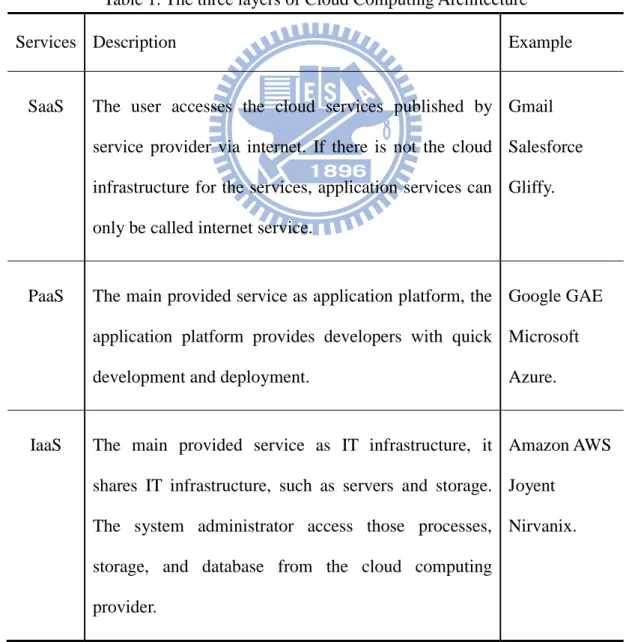
Cloud computing provides the computing power, the software services, and the storage space for the clients via internet anytime and anywhere. It is a model of supplement, consumption, and delivery for IT service, and also involves the provision of dynamically scalable and virtualized resources [14][3]. Cloud computing environment makes the business software and data stored on remote server ease-of-access by the Internet [2]. That usually utilizes the web-based protocol to let the client access through the web browser [9]. It includes three layers of service: Infrastructure as a Service, Platform as a Service, and Software as a Service [16], as the following Table 1.
Table 1. The three layers of Cloud Computing Architecture
Services Description Example
SaaS The user accesses the cloud services published by service provider via internet. If there is not the cloud infrastructure for the services, application services can only be called internet service.
Gmail Salesforce Gliffy.
PaaS The main provided service as application platform, the application platform provides developers with quick development and deployment.
Google GAE Microsoft Azure.
IaaS The main provided service as IT infrastructure, it shares IT infrastructure, such as servers and storage. The system administrator access those processes, storage, and database from the cloud computing provider.
Amazon AWS Joyent
2.2 Web Service and Web Service Composition
Web services are internet based software components which have the capabilities of cross-platform and cross-language. The W3C has defined “Web Service” that "a software system designed to support interoperable machine-to-machine interaction over a network. It has an interface described in a machine-processable format (specifically Web Services Description Language WSDL). Other systems interact with the web service in a manner prescribed by its description using SOAP messages, typically conveyed using HTTP with an XML serialization in conjunction with other Web-related standards." [4] The W3C has also pointed out that "We can identify two major classes of web services, REST-compliant Web services, in which the primary purpose of the service is to manipulate XML representations of Web resources using a uniform set of stateless operations; and arbitrary Web services, in which the service may expose an arbitrary set of operations." [22]
And the aim of web service composition (WSC) is to composite diverse web services to accomplish the request which cannot be satisfied by single web service. The Web services composition have static or dynamic way to be done. The static web service composition is constructed to solve the particular problem through identifying manually the capability of web services. That is composited by a series of known web services and a set of know data to obtain the expected results. Dynamic web service composition is to automatically select web services and flexibly composite those web services during the execution time. The aim is to build the automated service discovery and execution mechanism.
The web service composition is commonly described by using the Web Services Business Process Execution Language (BPEL) [21], it is defined by XML-based language that provides particular functionalities for processes, such as define
variables, create conditionals, design loops, and handle exception. And it utilizes web services as the model for the decomposition and the composition of the process. However, BPEL promotes the developing of workflow and the integration of business process.
Dynamic web service composition is the generation of dynamic composition of multiple web services to satisfy the user’s requirements, which is one of the most important areas of current web service research. Now most researches on web service composition focus on developing new approaches based on AI planning. That assumes the web services as actions, AI planning techniques are utilized for dynamic service composition by solving the service composition as the planning problem. Examples of the AI planning techniques include [18][10][8][13][15][6]. The task of WSC usually assumed that the composition process generates a composition workflow, which starts from the known variables to the expected goal. As an example in AI Planning Graph [18] utilizes graph algorithm based some strategy to generate service workflow. It constructs a compressed composition search space, and can obtain a solution in polynomial time, but with redundant services. As examples, the planning for WSC such as [10][13][6] , They utilize higher-level process models and constraints to decompose the model to an atomic-level composition for solving WSC problem. Web service composition techniques provide methodologies for compositing multiple services to satisfy the user request, which cannot be achieved by one single service.
2.3 Semantic Web and Semantic Similarity
information’s semantic and meaning on the World Wide Web [5]. It utilizes the machine-readable metadata to describe the human-readable information. That makes machines enable to infer the relation of the information. The machines process the information more intelligently and more precisely. Berners-Lee published “The Semantic Web” in Scientific American Magazine [1], which defined the Semantic Web as "a web of data that can be processed directly and indirectly by machines". It described the evolution of Web, as that semantic web makes largely data and information directly manipulate by machines without human interpretation. In the article, Berners-Lee also introduced “ontology” into the semantic web. With ontology, the machine has more capability of handling the meaning of lexical and semantic in the web. It is utilized to define and reason about domain knowledge.
The aim of semantic similarity is to measure the similarity between concepts, and it is different from measuring the similarity between words [12]. Semantic similarity is based on the concept relationships of ontology without additional corpus. Ontology is formal specification of the concept model, which contains concept, entity of objects, their property, restriction, and relation. It can use to describe the knowledge of application field as a set of concepts and relationships between concepts. With ontology, computer is more capable to process the lexical and semantic meaning. The followings define ontology hierarchical structures.
1. Concept Semantic Distance: Calculate the shortest path length between two concepts, denoted as l(ci, cj).
2. Concept Semantic Depth: Represent the depth of the concept from the top node, denoted as h(c).
3. Concept Semantic Coincidence: From the common ancestor between two concepts, calculate the number of intersection nodes and the number of
union nodes to obtain the ratio of the intersection to the union, denoted as
c(ci, cj). P(c) represent a set of concepts which is c is child concept. Than
c(ci, cj) is presented as:C(𝑐𝑖, 𝑐𝑗) =
|P(𝑐𝑖)∩P(𝑐𝑗)| |P(𝑐𝑖)∪P(𝑐𝑗)|
4. Concept Semantic Density:From the layer of the closest common ancestor between two concepts nodes, calculate the ratio of the number of child concept nodes to the count of layers which those nodes cross, denoted as
d(ci, cj).
2.4 Planning Graph
Planning graph techniques are studied in the AI planning domain. The planning graph provides a very powerful search space to improve the efficiency of AI algorithms. It is a layered graph whose edges are only allowed to connect two nodes from one layer to next layer. And the planning graph’s layers are with an alternating sequence of action layer and proposition layer. The proposition layer contains a finite set of states, and the action layer contains a finite set of actions (the action has preconditions, negative effects, and positive effects).
At the first layer of planning graph, P0, is a proposition layer which contains the
initial states of the planning problem. The next layer, A1, is a action layer which
contain a set of actions which preconditions can be satisfied by P0, and P1 is the union
of the states of P0 and the effects of all A1’s actions. Those preconditions of actions in
A1 are connected to the state nodes in P0 byincoming arcs, and those positive or
negative effects in P1 are connected to the state nodes in P1 byoutgoing arcs. The
2.5 Web Services Generation Tool for Service Composition
WSBen is a novel benchmark tool for web service composition and discovery, which provides a set of functions to simplify the generation of web service test sets, and build test environments including the testing requests [11]. The main contributions is to provide three different types of network models such as “random”, “small-world”, and “scale-free” network types. It also can generate diverse sizes of test data sets based on the network type you specify. At higher perspective, a web service can be assumed to be a transformation between two difference domains, which could be regarded as clusters of parameters. The development of WSBen is based on the above assumption. The network topology will be constructed as a directed graph based on graph theory. Each node is represented as a parameter cluster, and each edge is represented as a connecting between two different clusters, that will be regarded as generation template of web service.
There is an input framework that user can specify the generated web service and the characteristics of network topology in WSBen. The input framework 𝑥𝑇𝑆 = 〈|𝐽|, 𝐺𝑟 , 𝜂, 𝑀𝑝, |𝑊|〉. 𝑥𝑇𝑆 is described in the following.
1. |𝐽| is the total number of parameter cluster.
2. Gr donates a graph model to specify the topology of parameter cluster network.
The three types of network, which are “random”, “small-world”, and “scale-free” complex networks, can be simulated by the three network model, as following.
Erdo-Renyi (|𝐽|, 𝑝):
The model has such a simple generation approach that it creates | J | nodes in graph and chooses each of edges in the graph with probability p.
Newman-Watts-Strogatz (|𝐽|, 𝑘, 𝑝):
The initialization is a ring graph with k nodes. And then each node adds to graph and construct edge connected others with probability p, until there are | J | nodes in this graph
Barabasi-Albert (|𝐽|, 𝑚):
There are m nodes with no edges in the initial graph. Each node adds with m edges, which are preferentially attached to existing nodes with high degrees.
3. 𝜂 donates the parameter condense rate. Users can control the density of partial matching cases in generated web services.
4. 𝑀𝑝 donates the minimum number of parameters in a cluster. In other word, each cluster has at least 𝑀𝑝 parameters.
Chapter 3 A Novel Mechanism for Semantic Web Service
Composition in Cloud Computing
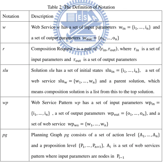
In this chapter, we introduce our novel composition framework, a semantic web service composition in Cloud. In Section 3.1 we identify our problem. In Section 3.2 we will introduce the overview of proposed service composition mechanism and each step of mechanism. In Section 3.3, we have discussions about possible advantages and disadvantages of proposed mechanism. In this chapter, we use some symbol to express the proposed mechanism. That are illustrated and defined as following table.
Table 2. The Definition of Notation Notation Description
w Web Service w has a set of input parameters win = *i1, … , in+ and a set of output parameters wout = *o1, … , on+
r Composition Request r is a pair of 〈rin, rout〉, where rin is a set of input parameters and rout is a set of output parameters
slu Solution slu has a set of initial states sluin = *i1, … , in+, a set of web service sluw = *w1, … , wn+ and a parent solution, which
means composition solution is a list from this to the top solution.
wp Web Service Pattern wp has a set of input parameters wpin = *i1, … , in+ , a set of output parameters wpout= *o1, … , on+, and a set of web service wpws = *w1, … , wn+
pg Planning Graph pg consists of a set of action level *A1, … , An+ and a proposition level *P1, … , Pn:1+, Ai is a set of web services pattern where input parameters are nodes in Pi;1
∩ s1s2 The amount of same concepts between s1 and s2, where s1 and s2
both are sets of concepts.
∪ s1s2 The amount of different concepts between s1 and s2, where s1 and
s2 both are sets of concepts.
𝛼 The variable 𝛼 represents the weight on parameter matching in matching score.
𝐾𝑀 KM Represent Kuhn-Munkres algorithm which solves the
assignment problem in polynomial time. That assigns the output parameters of one service to input parameters of another service. Sim(c1, c2) The similarity value between two concepts.
3.1 Problem Definition
In this thesis, our main goal is to solve the existed problems of service composition. Our focused problems include that service composition is essentially an error-prone process, the solution of service composition is always complex, and the request is hard to find the exact solution. Those problems are described in the following.
1. When the request is more complex, it always takes much time and finds the solution which is quite complex and resource-consuming. It means that the solution uses very large amount of services to satisfy the request.
2. Sometimes, there is no solution which exactly corresponds to the request. It is lack of flexibility to provide an approximate solution. If the solution is complicated, whether can find approximate solutions instead.
3. The problem of service composition is an error-prone process. It needs an effective mechanism which can provide multiple solutions to avoid that. To recommend a list of suited service compositions for selection or to evaluate from those solutions.
Thus, service composition algorithm may encounter above situations, and those problems are our focused issues.
3.2 Web Service Composition Mechanism
In this section, we will introduce the proposed service composition mechanism which includes four steps, such as preprocessing, service pattern matching, service composition, and search optimal solution. Those modules will be described in following subsections. At first we will introduce the overview of the mechanism, and then we will introduce each step of the mechanism.
3.2.1 Overview of the proposed mechanism
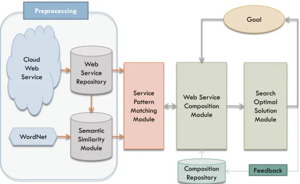
For improve the current web service composition mechanisms based on forward strategy, we proposed the framework including Service Pattern Matching Module, Web Service Composition Module, and Search Optimal Solution Module. Figure 1 shows that the flow diagram of the proposed mechanism. Service matching module is used to provide services for the query of service composition module. Service composition module provides multiple solutions for Search optimal solution to choice the best suited solution.
Figure 1 .The flow diagram of the service composition mechanism
The flow diagram of the proposed mechanism is shown in Figure 1. The flow diagram has the following 4 steps:
1. There are two parts in this step. One is the web service repository, and the other is semantic similarity module. The web service repository will search web service form distributed UDDIs in Cloud and store those service to repository database. All web services in repository will be updated regularly. Semantic Similarity Module pre-calculates the semantic similarity values between any two concepts and stores the similarity values into semantic similarity database for querying.
2. Service Pattern Matching Module utilizes Web Service Repository and Semantic Similarity Module to select the suited web services corresponding to the query, and group them by similarity of web services. It will provide a set of service groups for service composition.
Web Service Composition Module Search Optimal Solution Module Composition Repository Goal Preprocessing Web Service Repository Semantic Similarity Module Cloud Web Service WordNet Service Pattern Matching Module Feedback
3. Service Composition Module will query Service Pattern Matching Module to get services which are required by composition algorithm. Service Composition Module will generate multiple service composition solutions according to the goal.
4. According to the given goal, Search Optimal Solution Module will calculate the score of each solutions and choice the most suited web service composition from these found solutions
Those steps are the progress of our mechanism. The following subsection will explain how to get solutions by Service Composition Module and how to choice the best solution by Search Optimal Solution.
3.2.2 Preprocessing
In web service composition, the times of querying services is a great quantity. If you query web services registered in distributed UDDIs at runtime of service composition, the processing efficiency is obviously lower than web services stored in one centralized database. All web services will be stored to the structured Web Service Repository. Otherwise, the calculation of semantic similarity between concepts is time-consuming, that will be preprocessed by Semantic Similarity Module. Service Pattern Matching Model according the repository and the relationships of concept similarity to response the query.
The preprocessing includes two parts: 1. Web Service Repository
The aim of service repository is to virtualize service discovery. We query web services registered in distributed UDDIs in cloud and parse the WSDL
of web services to store into repository database, as shown in Figure 2. It will search regularly web services from distributed UDDIs and analyzes the structure to update database. The structure includes a set of input parameters, a set of output parameters, and service name. It is helpful and flexible to composite web service.
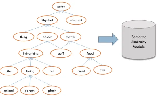
2. Semantic Similarity Module
The semantic module is for discovering the relationship between web services. According to the definition of lexicon and classification on WordNet, transform it into the concept and relationship of Ontology, as shown in Figure 3. And we calculate the similarities between concepts. The calculation of semantic similarity is described in Chapter 2. Through these functions, we can obtain semantic similarity values between semantic concepts. Those value’s ranges are between 0 and 1, and the higher value represents higher similarity. We pre-calculate those similarity values, and store into database.
UDDI UDDI UDDI UDDI UDDI WS WS WS WS WS WS WS WS WS Web Service Repository
Figure 3. Import semantic concepts from WordNet
3.2.3 Service Pattern Matching Module
This section will introduce service selection mechanism. In Cloud, there are so many similar web services, it causes that solution space expands quickly, so we could consider that similar web services as one. “Service pattern” is a concept that we proposed in this algorithm, which means that group those web services by the similarity of the input parameters and output parameters. A service pattern includes a set of web services and those included web services can be presented by this pattern. This module will provide service patterns according to the request.
Service pattern matching algorithm includes three steps: 1. Semantic Parameter Expansion
Semantic expansion is based on sematic similarity module (SSM), which records relationships between semantic concepts. Querying the SSM according to the request, it will get a set of concepts which are similar with the request. Add those similar parameters to quest set of web service.
entity
Physical abstract
object
thing matter
living thing stuff food
life being cell
animal person plant
meat fish
Semantic Similarity Module
2. Query Web Service Repository
From previous step, we will have a set of parameter query. We query the services, whose output parameters can provide one of query parameter set, from repository. Then we can find web services which provide the expected output.
3. Extract Web Service Pattern
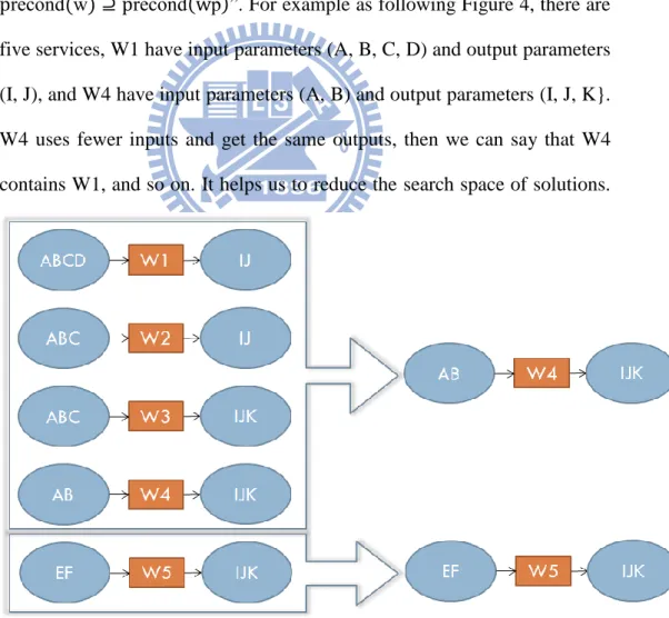
In the step, we collect a set of web services from previous step. We group those web services, and each group can be represented by one service in its group. The extraction rule of service pattern is “effect(w) ⊆ effect(wp) ∧ precond(w) ⊇ precond(wp)”. For example as following Figure 4, there are five services, W1 have input parameters (A, B, C, D) and output parameters (I, J), and W4 have input parameters (A, B) and output parameters (I, J, K}. W4 uses fewer inputs and get the same outputs, then we can say that W4 contains W1, and so on. It helps us to reduce the search space of solutions.
3.2.4 Web Service Composition Module
In the section, we will introduce composition mechanism we proposed in this thesis. In our proposed algorithm we use planning graph based on backward strategy to solve the problem of huge search space. The aim of backward search is to find the initial states, so we propose an algorithm for solution extraction of planning graph, which help us to find the initial state. Web service composition module includes four steps:
1. Expand the planning graph
In this step, we will expand the planning graph to one more action level with backward search. From the last proposition level in planning graph, we can get a list of expected parameters, and then query service pattern matching module (SPMM) to get service patterns. Add those service patterns to new action level, and arrange new proposition level. The Algorithm ExpandBasedOnBackward is shown in Appendix.
2. Extract solutions from the planning graph
From previous step, we can get planning graph which contains one more level. We need to trace the possible solutions from the planning graph. So we keep those lists of service composition, and we extend those compositions with that new level. We find out the service combinations to extend the service compositions from the action level. That is for finding solutions which correspond to the initial state of the request. The Algorithm ExtractSolutions is shown in Appendix.
3. Reduce solutions
We have a set of service compositions from extracting solutions, And we will utilize two strategies to reduce solutions. One of the strategies is that remove the solutions which utilize service more than threshold in the new extended level. The other is to remove the similar solution. They help us to decrease the complexity and quick growth of solutions. The Algorithm ReduceSolutions is shown in Appendix.
4. Validate solutions whether correspond to user request
From the previous step, we will have a set of solutions to calculate the score to find the best solution. If there is not solution correspond to user request, then expand the planning graph to next level. Repeat the above steps until find at least one solution. The Algorithm ValidateSolution is shown in Appendix
Here we give another example to explain our proposed composition mechanism. Assume a user request which has been a set of input parameter rin = *A, B, C, D+ and a set of output paramters rout= *M, N+. And there are nine web services in our web service repository. The following Table 3 shows the details of example web service repository.
Table 3. The example of web services
Web Service Input Parameters Output Parameter
W1 A,B,C E,F W2 A,B H W3 D,E I W4 E,F J W5 K,L W6 G I W7 H M W8 I,J,K M,N W9 L N
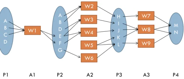
Through the expansion algorithm, based on backward strategy, of web service composition, we will get the planning graph which has user request at the first proposition level and the last proposition level. The following Figure 5 shows the result.
Figure 5. The simplified planning graph for the above example
A B C D M N W8 H I J K L W1 W3 W4 A B D E F G W5 W9 W6 W7 W2 A1 A2 A3 P1 P2 P3 P4
{A, B, C, D} and {M, N} are the input and output parameters of the composition request. At first, we search web service which can output {M, N}, then we get *w7, w8, w9+ which can support the proposition 4, our goal. Those three web service
will be involved in action 3. We collect input parameters of web service in action 3, and we will get proposition 3. The rest of proposition and action are like this, and so forth.
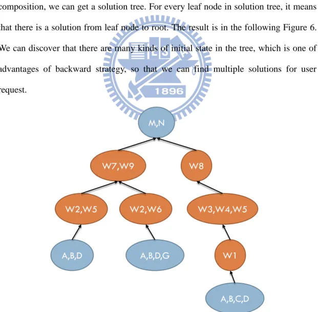
From the previous step, we have a planning graph, and it needs us to extract solutions. We utilize our proposed algorithm to extract solutions, and will get a tree structure, which is for tracing solution. Through the extracting solution of web service composition, we can get a solution tree. For every leaf node in solution tree, it means that there is a solution from leaf node to root. The result is in the following Figure 6. We can discover that there are many kinds of initial state in the tree, which is one of advantages of backward strategy, so that we can find multiple solutions for user request.
Figure 6. The solution tree for the planning graph for the above example.
M,N W7,W9 W8 W3,W4,W5 W2,W5 W1 A,B,D A,B,C,D W2,W6 A,B,D,G
{M, N} are the output parameters of user request. It is located in proposition 4, so we need to find the combinations of web services in action 3, which can correspond to {M, N}. And we will get two combinations, which are {W7, W9} and {W8}. Those combinations will be added to the root as its child. Now there are two nodes at second level. The solution node composited by {W7, W9} requires a set of input parameters {H, L}, so we need to find the combinations of web services in action 2, which can correspond to {H, L}. So we get {W2, W5} and {W2, W6}, and so forth.
3.2.5 Search Optimal Solution Module
After establishing the solution tree, we get service composition solutions which possibly satisfy user request. In this section we will introduce search optimal solution mechanism how to score those solutions and pick up the highest score solution.
At first, we calculate how precise the solutions correspond to the user request. We utilize the ratio of the number of intersection to the number of union, where are between the solution’s initial states and the user request’s inputs. The precision equation is in the following.
Precise(s1, s2) =
∩ s1s2
∪ s1s2 (1)
Equation (1) shows the precision. ∩ s1s2 represents the amount of same concepts and ∩ s1s2 represents the amount of all different concepts, where S1 and S2 both are lists of concepts. This equation evaluates how precise between the goal and the solution and how different between two lists of concepts.
After previous step, we have the precise of solutions. For calculation of the score of each solution, we need to calculate how matching between the levels of the solution. The matching equation is in the following.
Mat(s1, s2) = (KM − α(∪ s1s2−∩ s1s2))
where KM = KM(〈Sim(c1, c2)〉 (c1 ∈ s1, c2 ∈ s2) (2)
Equation (2) shows the matching score. In above equation, KM represents classical Kuhn-Munkres algorithm which solve the assignment problem, and Sim represents the similarity between any two concepts in s1 and s2. This equation is to
evaluate the matching score of two solutions.
With the previous two formulas, we can calculate the solution score. It sums the matching scores between levels of the solution and divides by the number of levels to get the average. Than we get the average of matching score, and multiple by the precision of the solution and the request. The score equation is in the following.
Score(slu) = Precise(slu. in, r. in) ∑ Mat(s1, s2)
slu s1,s2
𝑛 (3)
Equation (3) shows the solution score. Solution slu is a list of nodes from node leaf to the root, which represent each level of service composition, and the number of levels represents as n. The Precision is to calculate how precise between the input parameters of the request r and the input parameters of the solution. The equation is to evaluate at the score of service composition solution.
3.3 Discussion
Our proposed mechanism is suitable for service composition due to the problems that service composition is an error-prone process, and the solution is always complicated. In this thesis, we designed the mechanism suited for finding multiple service compositions to overcome the above problems. Sometimes the exact solution is not existed or more complicated, and our proposed mechanism still can recommend approximate solutions. Therefore, our proposed service composition mechanism can recommend the most suited solution from multiple solutions.
On the other hand, In order to provide multiple solutions, it must need to trace each possible solution. Our proposed mechanism can limit and reduce the growth of tracing solution to avoid exponential growth. If the growth is beyond the capability of our algorithm, that will growth exponentially.
Chapter 4 Simulation Results and Analysis
In this chapter, we introduce our simulation environment and present the simulation results. At first, we describe simulation environment, design, assumption, and performance metrics. Then, the simulation results include effectiveness and efficiency analysis, by implementing the proposed mechanism. Moreover, there is a discussion in the end of this chapter.
4.1 Simulation Environment
The simulation platform environment is described first in section 4.1, and then to show that how the simulation is designed. Finally, assumptions, definition of cases, and performance metrics are introduced.
4.1.1 Simulation Design
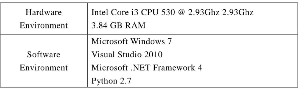
We established a simulation platform by the proposed mechanism for validating our algorithm. In this platform, we utilize WSBen [11], which is widely used to evaluate the efficiency and effectiveness in web service discovery and composition, to generate different test sets for validating our algorithm. The simulation platform will carry out the algorithm according to the test data set and request from WSBen. The following Table 4 describes the environment details of the simulation platform.
Table 4. Simulation Platform Environment Hardware
Environment
Intel Core i3 CPU 530 @ 2.93Ghz 2.93Ghz 3.84 GB RAM
Software Environment
Microsoft Windows 7 Visual Studio 2010
Microsoft .NET Framework 4 Python 2.7
Figure 7. The Architecture of Simulation Platform
The architecture of simulation platform is shown in Figure 7. WSBen build the test data for WSC algorithm, including a set of web services and a set of feasible requests. In our simulation, we parse the web service generated from WSBen, then store information into the web service repository. The information is including service name, input parameters, and output parameters. Service pattern matching module takes charge web services selection according to the service query from web service composition module. In addition, it also groups the selected web services as web service patterns for composition algorithm. Each of web service patterns includes a list of web services, which can be expressed by one pattern reducing similar services. Web service composition module conducts the composition algorithm according to the composition request, which interacts with service matching module during the processing until getting solutions. It will generate a list of candidate solutions of web service composition. Search optimal solution module calculates each score of candidate solution, and generates a recommendation list.
Web Services
Composition Solution Request
4.1.2 Simulation Assumption
The assumptions in data sets for simulation have to describe in advance. First is that there are three types of network in the simulation, which are random, small-world, and scale-free types. And each of networks is assumed as parameter cluster network, and web service is a transformation between two clusters. Each cluster contains parameters, and it is also called domain. WSBen provides a set of functions to simplify the generation of test data for WSC algorithm. It generates web services according to the parameter cluster network which user specify. In our simulation, we assume that there are 100 clusters in network and the parameter condense rate is 0.8. Three types of network models (mentioned in Chapter 2) are as follows:
1. Random Network: Barabasi-Albert (100, 0.06)
The model creates 100 nodes in graph and chooses each of edges in the graph with probability 0.06.
2. Small-World Network: Newman-Watts-Strogztz (100, 6, 0.1)
The initialization is a ring graph with 6 nodes. And then each node adds to graph and construct edge connected others with probability 0.1, until there are 100 nodes in this graph
3. Scale-Free Network: Erdo-Reyi (100, 6)
There are 6 nodes with no edges in the initial graph. And then each node adds with 6 edges until reach 100 nodes. Each added edge is preferentially attached to existing nodes with high degrees.
For each network, there are 10 different sizes in each of test data types, which sizes are 10,000 to 100,000, respectively. Thus, there are 30 test sets (three frameworks multiplied by ten different test sizes) in our simulation.
4.1.3 Performance Metrics
Effectiveness, efficiency, and feasibility are three evaluations, which used to test our proposed approach. We use diverse sizes of web services and three types of web service networks to measure how scalability and robust our approach is. The evaluation metrics are as follows.
1. #T: It measures how long an algorithm spends to find a physical solution or approximate solution. In other word, this is a measure of computational efficiency.
2. #C: The number of web services in a solution of web service composition problem. This is a measure of effectiveness.
3. #L: The number of levels of web services in a solution of web service composition problem. This is also a measure of effectiveness.
4. #P: It measures how precise an algorithm finds solution corresponding to the request. It means that a solution is physical solution if it has precision 100 precision, otherwise it is an approximate solution. Precision (described in Equation 1) is a measure of effectiveness.
4.1.4 Simulation Cases
Three cases are designed in the experiment to observe our proposed mechanism in comparison with traditional forward graph planning approach for web service composition problem. The different dataset types of web service generation for 3 cases are case 1) random network, case 2) small world network, and case 3) scale-free network. Besides, we also give statements and comparisons for the most two important evaluations, effectiveness and efficiency, of proposed mechanism in experiment results. One is the effectiveness evaluation which includes the cost, the
number of level, and the precise. The other is the efficiency evaluations which compare by the time of finding solution.
4.2 Simulation Results and Analysis
In section 4.2, we show the efficiency, effectiveness, and feasibility of out proposed algorithm in three cases. We utilize diverse sizes of web services and different type of network topology to observe the scalability and robustness of our proposed algorithm. Some related results are illustrated in the below sections. The three test data sets of our experiments deal with the networks of random, small, and scale-free type. We compare backward strategy with forward strategy to observe the results. The results are shown in the following tables.
4.2.1 Case 1: Random network
The following Table 5 shows the results of five requests of random network with 10,000 web services. Backward and Forward both can find solutions in all cases. Regarding #Level, Backward and Forward have no difference to find solution. Although Backward takes more time than Forward, in the number of web services, our proposed Backward outperforms the Forward. We use less 20 services to fulfill the request in all cases, but the Forward use more than 200 web services to find solution.
Table 5. Results of random network with |W| = 10000 test request Backward Forward #L #C #T #P #L #C #T #P r1 8 18 2.725 1 8 262 1.033 1 r2 8 14 3.028 1 8 237 1.05 1 r3 7 9 1.916 1 7 220 1.066 1 r4 7 10 2.191 1 7 245 1.072 1 r5 9 16 4.141 1 9 241 1.062 1 Avg. 7.8 13.4 2.8 1 7.8 241 1.056 1
4.2.2 Case 2: Small world network
The following Table 6 shows the result of five test request of small world network with 10,000 web services. Both our proposed Backward and the Forward still can find solutions in all cases. Regarding #Level, the Result of Backward is as good as the Forward. Our proposed Backward take more a little time than the Forward, but in terms of #WS shows much better performance than the Forward. It means that using our proposed algorithm you can take more time to obtain much better solutions in small world network.
Table 6. Results of small world network with |W| = 10000
test request Backward Forward #L #C #T #P #L #C #T #P r1 14 14 1.599 1 14 183 0.863 1 r2 11 11 1.016 1 11 175 0.769 1 r3 12 12 1.985 1 12 156 0.746 1 r4 10 10 2.419 1 10 174 0.716 1 r5 16 16 1.854 1 16 181 0.903 1 Avg. 12.6 12.6 1.776 1 12.6 173.8 0.8 1
4.2.3 Case 3: Scale-free network
The following Table 7 shows the result of five test request of scale free network with 10,000 web services. The Forward still can solved all request, but use more than 200 web services to obtain solution. In the more complex scale-free network, although we cannot find the physical solution in some cases, we can find the approximate solution, which use much less services to satisfy the request.
Table 7. Results of scale-free network with |W| = 10000
test request Backward Forward #L #C #T #P #L #C #T #P r1 4 11 1.232 0.933 4 244 2.48 1 r2 4 6 3.151 1 4 343 1.654 1 r3 5 11 2.886 0.778 5 356 2.824 1 r4 - - - - 4 313 1.414 1 r5 4 10 0.203 0.814 4 281 2.122 1 Avg. 4.25 9.5 1.868 0.8812 4.4 316 2.3808 1
From above experiments, we use diverse test data sets to understand how different network to influence the performance of service composition. In general our proposed algorithm have much better performance in term of #WS. To compare diverse sizes of test data sets, we use charts to express the results, which are shown in the following.
4.2.4 Effectiveness and Efficiency
There are two parts in section 4.2.4. The one is result for effectiveness, and the other is result for efficiency. We compare the proposed mechanism with the traditional service composition mechanism to observe the proposed mechanism. Those two parts will be described in the following.
(1) Effectiveness
The major experiment metrics are #C, #L, and #P. We utilize diverse test data sets to observe our proposed algorithm based on backward strategy, to understand how diverse sizes of data sets to influence the effectiveness of service composition.
Figure 8. The average cost of finding solution with both methods in Random Network
0 50 100 150 200 250 300 350 400 450 10000 20000 30000 40000 50000 60000 70000 80000 90000 100000 #C |W| Backward Forward
Figure 9. The average cost of finding solution with both methods in Small World Network
Figure 10. The average cost of finding solution with both methods in Scale-Free Network
As shown in Figure 8, Figure 9, and Figure 10, we can observe that our proposed
0 50 100 150 200 250 300 350 400 450 10000 20000 30000 40000 50000 60000 70000 80000 90000 100000 #C |W| Backward Forward 0 50 100 150 200 250 300 350 400 450 10000 20000 30000 40000 50000 60000 70000 80000 90000 100000 #C |W| Backward Forward
cases. Because of the aim of Forward algorithm, which is to reach the goal as quick as possible, it expands the services as it can despite of the redundancy of web services. Our backward algorithm have no redundant web service existed in the solution, because its backward strategy search what it needs to reach the initial state. Figure 10 shows average cost of searching solution in Scale Free Network. It can be observed that the forward algorithm represent an unstable circumstances in Scale Free Network, when the size of a test data set become large. However, our backward algorithm is still to appear stable and effective results. On average, our algorithm reduces the 94% service cost for finding the solutions.
From the above charts, we have a simple deduction that the backward search will continue display the stable and smooth results in different types of network topology, even if the sizes of web services continues to increase.
Figure 11. Level of searching solution with both methods in Random Network
4 6 8 10 12 14 10000 20000 30000 40000 50000 60000 70000 80000 90000 100000 #L |W| Backward Forward
Figure 12. Level of searching solution with both methods in Small World Network
Figure 13. Level of searching solution with both methods in Scale Free Network
As shown in Figure 11 and Figure 12, it can be observed that there are same results which use the same number of levels to obtain the solutions in above two cases.
4 6 8 10 12 14 10000 20000 30000 40000 50000 60000 70000 80000 90000 100000 #L |W| Backward Forward 4 6 8 10 12 14 10000 20000 30000 40000 50000 60000 70000 80000 90000 100000 #L |W| Backward Forward
the others are almost same number of levels. The forward search aims to minimize the number of composition level to reach the goal, it means that the solution can be solved at least number of levels. Figure 11 and Figure 12 both get the same result in Random Network and Small World Network. It means that our backward algorithm also get the least number of levels to obtain the solutions. But in more complex Scale Free Network we use a little bit more number of levels to obtain solution. Although our backward algorithm uses a little bit more levels to get solution, we can obtain the solutions which use much less number of web services.
From the above three charts, shown in Figure 11, Figure 12, and Figure 13, we have a simple conclusion that the backward search in more complex network could obtain a little bit more levels of service composition. But it is acceptable that use a little bit more levels in exchange for low cost of services. The results in increasing web service are represented the stability as the forward algorithm.
Figure 14. Precision of searching solution with both methods in Random Network
50% 60% 70% 80% 90% 100% 10000 20000 30000 40000 50000 60000 70000 80000 90000 100000 #P |W|
Precision
BackwardFigure 15. Precision of searching solution with both methods in Small World Network
Figure 16. Precision of searching solution with both methods in Scale Free Network
As shown in Figure 14 and Figure 15, it represent that our proposed algorithm
50% 60% 70% 80% 90% 100% 10000 20000 30000 40000 50000 60000 70000 80000 90000 100000 #P |W|
Precision
Backward 50% 60% 70% 80% 90% 100% 10000 20000 30000 40000 50000 60000 70000 80000 90000 100000 #P |W|Precision
Backwardcomplex Scale Free Network our backward algorithm could not find the physical solutions in some requests. We observe the composition in Scale Free Network and find out the solutions which have less number of levels and much more number of services. Our algorithm aims to avoid the situations which have much complex services in one level. Based on the above aim, we may ignore the exact solutions in our algorithm, but our algorithm still can obtain approximate solutions in the complex network, which still have high precision.
(2) Efficiency
We utilize the same data set to observe our proposed algorithm based on backward strategy, to understand the influence of performance by increasing the number of web service. And we compare our algorithm with the algorithm based on forward strategy with three different types of network topology. It is shown in the following figures.
Figure 17. Time of searching solution with both methods in Random Network
0 100 200 300 400 500 600 10000 20000 30000 40000 50000 60000 70000 80000 90000 100000 #T |W| Backward Forward
Figure 18. Time of searching solution with both methods in Small World Network
Figure 19. Time of searching solution with both methods in Scale-Free Network
As shown in Figure 17, Figure 18 , and Figure 19, it represents that the backward algorithm takes more time than forward to obtain the solutions in all cases. We
0 100 200 300 400 500 600 10000 20000 30000 40000 50000 60000 70000 80000 90000 100000 #T |W| Backward Forward 0 100 200 300 400 500 600 10000 20000 30000 40000 50000 60000 70000 80000 90000 100000 #T |W| Backward Forward
observe that different network types start to growth exponentially in Random Network and Scale Free Network, when the number of web services increases to certain number. It can divide into two parts, one is the number of web service less than 50,000, and the other is more than 50,000. We observe a liner growth in the part less than 50,000, and the other part is an exponential growth. But in Small World Network we can clear see that they both are liner. We go deep into study why the exponential growth at the number of web service more than 50,000. We find out that the space of solution quickly growth more than our algorithm can shrink. However, when the sizes of web service are less than 50,000, our backward algorithm had better effectiveness and nearly efficiency in all cases.
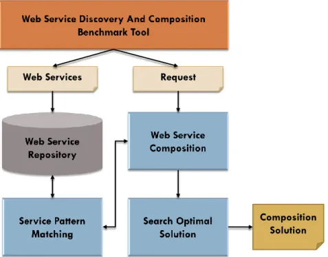
4.2.5 WSBen data set and general situation
WSBen[11] can build the test data for WSC algorithm, including a set of web services and a set of feasible requests. It is designed to generate the hardest solved request to validate the WSC Algorithm. That does not make the advantage of the proposed mechanism prominent. It is dedicated to find the approximate solution instead, which not exactly corresponds to the request but takes less service cost. Therefore, we design an example to explain the proposed mechanism in general situation. In the real world, people who composite services focus on what they want to know rather than what they can give. The advantage of backward search is to find the diverse initial states, which possibly match the user request. To find out what initial state can reach the goal, which user expects to know. We use the following Figure 20 to explain some situation which traditional composition mechanism cannot solve.
Figure 20. The example of solution tree
In Figure 20, there are two requests, which can represent the advantage, described in the following. One request is that the known input parameters are {A, B, C, D} and the expected output parameters are {L, M}. The traditional mechanism based on planning graph only can obtain the single path from the initial state {A, B, C, D} to the Goal {L, M}, which costs nine services to obtain the solution. The proposed mechanism based on backward can find out multiple paths which can reach the goal, as the above solution tree. In the mechanism, we can stop searching in finding the initial state {A, B, C, E}, if the user wants to find the approximate solution which have lower service cost and can give the expected output. The other request is that the known input parameters are {A, B, C} and the expected output parameters are {L, M}. According to the solution tree, there is no existed solution which can satisfy the request. The traditional composition mechanism can find the solution in this case, but the proposed mechanism can find the approximate solution instead.
traditional mechanism. From the above example, we can observe that the proposed finds many approximate solutions before finding the exact solution. If the composition requester can accept approximate solutions, the proposed mechanism does not take the total time for finding the exact solution. Also we can find approximate solutions at lower number of composition level. In the exponential growth composition space, if we could decrease one composition level, the time of obtaining solutions will dramatically decrease. From above example, we explain that the proposed mechanism can take less time to find acceptable approximate solution.
4.3 Discussion
In our experiments, we utilize three type of network topology and diverse sizes of web services to observe those two algorithms. The main findings about our proposed algorithm from the experiments are given as follows.
1. Effectiveness. The experiment results show our proposed backward algorithm has 94% better effectiveness compared to forward algorithm almost all cases. At few cases we use more little levels to obtain the solution, but we get low-cost solutions. As confirmed by the experiment results, our proposed algorithm also can get very high precise solutions almost all cases. 2. Efficiency. Although forward algorithm has better performance than backward algorithm, the cost of solution is high. Our proposed backward algorithm has nearly efficiency when the sizes of web service are less than 50,000. Also in random and small world network we can observe that our proposed algorithm do not growth exponentially when the size of test data increases.
Chapter 5 Conclusions and future works
This thesis emphasizes issues about service composition based on backward planning graph strategy. In this chapter, we summarize our studies and discuss our possible future work.
5.1 Conclusions
In this thesis, we proposed a semantic web service composition mechanism based on semantic in cloud environment. It utilizes planning graph based on backward search to find multiple feasible solutions, and recommends the best composition solution by the lowest using service cost. We also validated the proposed algorithm can improve the error-prone problem of service composition and the redundant web service involved in service composition. Therefore, the algorithm based on backward planning graph search, which is capability of recommending multiple service composition and remove the redundant services. As we can see the experiment results in chapter 4, we proved that our proposed backward algorithm had a better effectiveness than the forward search algorithm. The proposed algorithm is able to recommend approximate solutions of service composition using very few web services, because it has higher quality of relationships between services. In other words, we can decrease the amount of cost of web services and remain acceptable planning graph levels and execution time.
5.2 Future Work
In the future, we can study how to improve proposed greedy algorithm to expand the solution tree. To obtain right combinations is a very important issue for algorithm design. It can not only help to decrease wrong combinations, but also to improve the