二維cubic-k Dresselhaus-type 電子系統中在圓盤附近的量子散射

國 立 交 通 大 學

電 子 物 理 研 究 所

碩 士 論 文

二維 cubic-k Dresselhaus-type 電子系統中在圓盤

附近的量子散射

QUANTUM SCATTERING FROM

A CIRCULAR DISK IN A CUBIC-K DRESSELHAUS-TYPE

TWO DIMENSIONAL ELECTRON GAS

研 究 生：杜冠誼

指導教授：朱仲夏教授

附近的量子散射

QUANTUM SCATTERING FROM

A CIRCULAR DISK IN A CUBIC-K DRESSELHAUS-TYPE

TWO DIMENSIONAL ELECTRON GAS

研 究 生：杜冠誼

Student：Kuan-Yi Tu

指導教授：朱仲夏教授 Advisor：Prof. Chon Saar Chu

國 立 交 通 大 學

電 子 物 理 研 究 所

碩 士 論 文

A Thesis

Submitted to Department of Electrophysics

College of Science

National Chiao Tung University

in Partial Fulfillment of the Requirements

for the Degree of

Master

in

Electrophysics

July 2009

Hsinchu, Taiwan, Republic of China

二維 cubic-k Dresselhaus-type 電子系統中在圓盤

附近的量子散射

研究生：杜冠誼 指導教授：朱仲夏教授

國立交通大學

電子物理研究所

摘要

DSOI 貢獻的差異可以明顯地被辨識，同時得到所對應的能量耗散關係。在我們的發

現：對於linear-k Dresselhaus，電子自旋密度與機率密度分佈擁有空間對稱性

輪廓，與平面波入射角度無關。相反地，在 cubic-k Dresselhaus SOI 例子中明顯 地表示出與平面波入射角度相關。

特別地，若入射平面波角度為幾個特定的角度，我們可以發現有相似的電子 自旋密度對應在 cubic-k Dresselhaus 例子與 linear-k Dresselhaus 例子之 間。

TWO DIMENSIONAL ELECTRON GAS

Student: Kuan-Yi Tu Advisor: Prof. Chon-Saar Chu

Department of Electrophysics National Chiao Tung University

Abstract

This thesis work has devoted to the study of spin-dependent scattering effects from a circular-disk microscopic structure with Dresselhaus-type spin-orbit coupling. The Dres-selhaus spin-orbit coupling considered here includes both contributions terms for one is linear-k dependence and the other is cubic-k dependence.

Based on the method of partial waves, the complete scattering wave function in a circular scattering region can be rigorously derived and obtained. Through investigating their spatial-resolved scattering behaviors from linear and cubic Dresselhaus-type SOI disk under the electron plane wave incidence, different DSOI contributions can be appar-ently discerned, and their corresponding detail energy dispersion relationships as well. In our findings: for linear-k Dresselhaus case, the spin density and probability density distri-butions own their spatial symmetry profile, which is featured independence of the plane wave incident angle. On the contrary, strong incident angle dependence is manifested for the case of cubic-k Dresselhaus spin-orbit interaction.

In particular , for incidence plane wave in some characteristic angle, we can find similar spin density responses between cubic-k Dresselhaus case and linear-k Dresselhaus case.

iii 感謝朱老師兩年來教導，謹慎細密的研究態度與研究的熱忱，讓我獲益良多。也 感謝老王學長在研究中給我的協助與討論，唐志雄學長在關鍵的時期給予我最寶 貴的意見以及想法。多虧有實驗室夥伴興哥、fat、布達、小明、偉哥帶給我的 歡樂，才能在研究外有多餘的樂趣，也感謝實驗室夥伴對於我一些無理或固執行 為的包含。最後特別，感謝興哥在這兩年中對我人生的想法態度上的開導，讓我 無論對人對事多有一番體悟。謝謝我的家人，謝謝我的朋友，感謝所有幫助我關 心我的人。

Abstract in Chinese i Abstract in English ii

Acknowledgement iii

1 Introduction 1

1.1 Background : types of spin-orbit coupling system in solid state system . . 2

1.2 Motivation : cubic-k Dresselhaus spin-orbit interaction (SOI) . . . 3

1.3 A simple guide to thesis . . . 3

2 Two dimensional Dresselhaus-type SOI electron system 5 2.1 Linear-k Dresselhaus SOI . . . 6

2.1.1 Incident plane wave . . . 7

2.1.2 Cylindrical form representation of the eigenstates . . . 12

2.2 Cubic-k Dresselhaus SOI . . . 14

2.2.1 Incident plane wave . . . 14

2.2.2 Cylindrical form representation of the eigenstates . . . 17

2.3 Energy dispersion of Dresselhaus SOI system . . . 20

2.4 BIA in spin splitting in 2D systems . . . 24

2.5 Connection between linear-k DSOI and ROSI systems . . . 25 3 Scattering from a cylindrically symmetric potential in a Dresselhaus SOI

system 28

3.1 Cubic-k Dresselhaus SOI . . . 29

3.1.1 Coupled cylindrical wave representations of the incoming wave . . . 29

3.1.2 Coupled cylindrical wave representations of the outgoing wave . . . 31

3.2 Linear-k Dresselhaus SOI . . . 36

3.2.1 Coupled cylindrical wave representations . . . 36

3.3 Scattering of the scattering state . . . 39

3.4 Spin density of the scattering state . . . 39

3.5 Particle continuity equation . . . 41

4 Numerical results and discussions 44 4.1 Results for linear-k Dresselhaus SOI . . . 44

4.2 Results for cubic-k Dresselhaus SOI and more Discussions . . . 48 4.3 Discussion on the connection of spin density with the plane wave direction 49

5 Future work 50

A Simplify the boundary condition problem 51 B Derivation of spin density of the total wave function after scattering 55 C Comparison of analytical results and numerical approach for cylindrical

2.1 Radial profile of ”hard” wall disk of our system. . . 8 2.2 Energy dispersion with helicity η for a linear-k Dresselhaus system ; the

blue line correspond to η = + and the red line correspond to η = −. The dash line means that system has no spin-orbit coupling (β1 = 0) and

Eq. (2.5) represents two parabolic bands centered up k = −η(β1κ2)

2 . . . 9

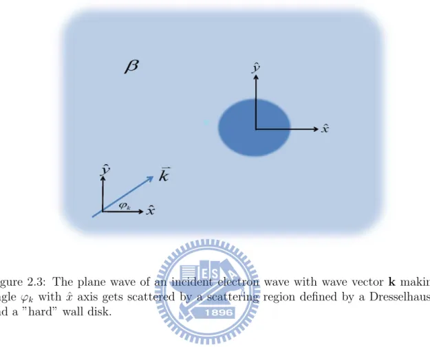
2.3 The plane wave of an incident electron wave with wave vector k making an angle ϕk with ˆx axis gets scattered by a scattering region defined by a

Dresselhaus SOI and a ”hard” wall disk. . . 10 2.4 Dispersion relation for a 2D Dresselhaus-type system (includes linear and

cubic terms) and the Dresselhaus constant β = 27eVAo3 _{and d = 15nm. . . 21}

2.5 Dispersion relation for a 2D Dresselhaus-type system (includes linear and cubic terms) and the Dresselhaus constant β = 27eVAo3 _{and d = 15nm in}

the larger k range. . . 22 2.6 The roots of the energy dispersion Eq. (2.35) where ϕk = π₃ and η = +.

The right pattern is the real part of k and the left pattern is the imagine part of k. In the central region of the real k and k imagine pattern show that the three roots in the region are all pure real values. Apparently, the momentum k we have to neglect is only the smallest one due to the corresponding much fast oscillation and then the others are exactly we must consider. . . 24 2.7 the [x0_{, y}0_{] system is rotated by angle θ, retaliative to the [x, y] system. . . 26}

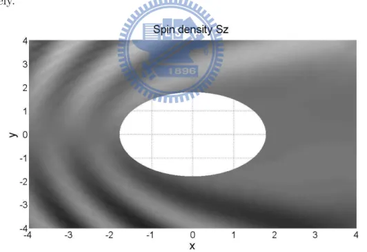
4.1 Distribution of the out-of-plane spin density Sz. The plane wave incident

a hard wall disk in linear-k Dresselhaus system with the helicity η = +, the incident energy ε=7.7, and the incident angle ϕk=0. Lighter regions

means the region whose spin density Sz >0 (spin up). And the darker

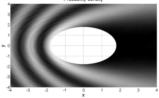
regions represent the region of spin down . . . 45 4.2 The spatial dependence of the magnitude of the total wave function

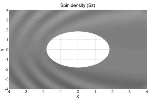
prob-ability density. Out of the white circle is the region with finite Dresselhaus SOI. Apparently, when the plane wave propagates along the x axis, the probability density is almost zero behind the disk due to the hard wall disk . 46 4.3 Distribution of the out-of-plane spin density Sz. The plane wave incident

a hard wall disk in linear-k Dresselhaus system with the helicity η = +, the incident energy ε=13.23, and the incident angle ϕk=0. Lighter regions

means the region whose spin density Sz >0 (spin up) . And the darker

regions represent the region of spin down . . . 47 4.4 The spatial dependence of the magnitude of the total wave function

prob-ability density. Out of the white circle is the region with finite Dresselhaus SOI. Apparently, when the plane wave propagates along the x axis, the probability density is almost zero behind the disk due to the hard wall disk. 47 4.5 The quality the spin density Sz determining the number m as function of

ϕ for a central hard wall disk where m represents the number of the partial

waves we must sum. Apparently, the line of the spin density corresponding to the distribution of the spin density Fig. 4.1 at r=2 is saturated for a larger m. And the probability density also has the same situation. . . . . 48 C.1 Comparison of analytical results and numerical approach for cylindrical

wave case of min=1: (a) N = 11, (b) N = 45, (c) N = 47 and (d) N = 49. 64

C.2 Comparison of analytical results and numerical approach for cylindrical wave case of min=3 : (a) N = 49 and (b) N = 51. . . 65

wave case of min=7: (a) N = 129 and (b) N = 131. . . 65

C.4 Comparison of analytical results and numerical approach for cylindrical wave case of min=11 : (a) N = 133 and (b) N = 135. . . 65

C.5 Comparison of analytical results and numerical approach for cylindrical wave case of min=1 : (a) N = 63 and (b) N = 65. . . 66

Introduction

The spin dependence of the electronic properties of mesoscopic technology and artificial nano-structure is one of leading problem nowadays in the physics of electric devices. In this way, taking account of spin property of electrons are the improvement of actual devices. To develop spintronic device in spintronics, quantum information, and other applications is necessary to understand how the transport of electron affect its spin and further control conditions on the manipulation of the spin orbit interaction in the semi-conductor macrostructure. The interaction causes the decay of spin polarization since the spin-orbit coupling breaks the total spin symmetry [1]. Accordingly, we must understand the spin-orbit coupling [2].

In semiconductor with strong SOI, the energy eigenstates are spin dependent and can have apparently spin splitting without a magnetic field for electrons when there exits inversion asymmetry. And then the effect in the low dimensional structure becomes larger where the inversion asymmetry controlled. It is known that in a variety of systems we consider that changing the spin properties of an incident beam of particle in scattering experiment. The spin-orbit interaction cause asymmetry of the differential scattering cross section ( skew scattering ). In addition, the SOI also changes the polarization vector of the incident beam.

in solid state system

There are two types of spin-orbit interaction in semiconductor according to the physical origan. One is intrinsic type such as Rashba spin orbit interaction (RSOI) [3] induced by structure inversion asymmetry (SIA) and the other is extrinsic type such as Drsselhaus spin orbit interaction (DSOI) [4] induced by bulk inversion asymmetry (BIA) of the crystal lattice. The effect produced by the interplay between Dresselhaus and Rashba spin-orbit interactions on spin relaxation has been studied in a few publications [5–7]. Furthermore , there are a few works on the transport properties of two-dimensional electron gas [8– 11] . Especially, Datta and Das proposed a spin-field-effect transistor (SFET) [12] for quasi-1D ballistic wires with Rashba coupling . In thin quantum wells, the strength of the DSOI is compatible to the strength of the RSOI. The special spin symmetry arises due to the translational invariance in the longitudinal coordinate in quantum wires is used to propose a transport experiment to measure the strengths of the Rashba and the Dresselhaus interaction for any chosen polarization [13]. There are a few works on the effects of the competition between two types of SOI on the transport properties in mesoscopic rings [14, 15].

A promising spin transistor application has been proposed that the strength of the RSOI can be tuned by external gates voltages or asymmetric doping and this initiated intensive research in spintronics [16]. Schliemann, Egues, and Loss proposed a SFET [17] that can operate in diffusive quasi-2D systems based on tuning Rashba and linear Dresselhaus terms to be equal in strength, which produces long spin lifetime , neglecting cubic Dresselhaus term. On the other hand, recent studies have been devoted to the physical consequences of the interplay of the RSOI and impurity [18]. Recently, the intrinsic spin Hall effect (SHE ) [19, 20] as been established in a spin-orbit coupled p-doped semiconductor and in a Rashba spin-orbit coupled two-dimensional electron systems was predicted theoretically.

1.2

Motivation : cubic-k Dresselhaus sporbit

in-teraction (SOI)

In quasi-2D systems, Dresselhaus terms has two components, one linear in the momentum and the other cubic. The cubic Dresselhaus contribution [21] is often neglected since it is smaller apparently than the linear Dresselhaus contribution. Nevertheless , the strength of the SO terms are difficult to measure so that to obtain a full understanding of their strength is crucial . In addition, in confined system such as quantum dot, quantum wire, some effect of the linear Dresselhaus SOI are suppressed, so it is important to know the contribution from the cubic Dresselhaus SOI which is helpful to develop spintronic devices. Theoretically, the spin current is the important physical quantity in spintronics, and it has been extensively studied [22–24] . Many fundamental phenomena, such as the SHE and the spin precession in systems with spin-orbit coupling have been discovered . There are many recent works on spin dependent quantum scattering [25] around microstructures [26–28]. In this thesis , we study the scattering of the scattering of electrons by a disk in 2DEG with Dresselhaus spin-orbit coupling.

1.3

A simple guide to thesis

In Chapter 2 , we will solve the eigenstate problem in two dimensional Dresselhaus-type system including linear-k and cubic-k DSOIs, so that the energy dispersion can be obtained. In addition , the eigenstates would be represented in cylindrical form due to the cylindrical symmetry potential .We consider that the plane wave which is the eigenstate of Dresselhaus-type Hamiltonian incident a hard wall disk in DSOI system. At such, we can make a connection between linear-k Dresselhaus and Rashba Hamiltonian.

In Chapter 3, we introduce the method of partial waves for a scattering. The total waves are composed of incoming waves and outgoing waves, where the incoming wave part is given by the incident plane wave and then outgoing wave part can be represented

contains unknown coefficients which are contributed from the two kinds of helicity wave functions. The unknown coefficients can be obtained by solving the boundary condition problems. Finally, we obtain the particle current density by driving the particle continuity equation of the Dresselhaus-type system .

In Chapter 4, the numerical results show the spin density or other quantities after scattering by a hard wall disk both in linear-k and cubic-k DSOI. Therefore, we can use the result to evaluate the cubic-k contribution during the scattering process by comparing the results only for linear-k Dresselhaus and the results includes cubic-k Dresselhaus. Also, we discuss the connection between spin density and the plane wave direction.

In Chapter 5, we present possible work about spin-orbit interaction in Dresselhaus or Rashba system.

Two dimensional Dresselhaus-type

SOI electron system

In this chapter we present a theoretical study of electron scattering in two dimensional Dresselhaus-type SOI electron system. Using the spin dependent method of partial waves [29] the complete scattering wave function is derived exactly for the case of a circular region. For a 2D central potential (hard wall disk), the cylindrical symmetry governs that the wavefunction is expressed most conveniently in polar coordinates. There exit linear-k DOSI and cubic-k DOSI in Dresselhaus-type SOI and mostly cubic-k DOSI is neglected. At the same time, linear-k DSOI can be compare with that Rashba-type spin orbit interaction (ROSI) that we can make a connection between them. The competition of two types of SOI on the transport properties of two dimensional electron gas are interesting and highly desirable.

In our numerical examples, physical parameters are chosen according to practical experimental situation and for the material GaAs. Parameters units typical for GaAs are: electron density n =2.51 × 1011_cm−2_{; energy units ε}∗ _{= 8.977 meV; m}∗ _{=0.067 m}

e;

Dresselhaus strength β∗_{= 4553 eVA}3_{; k}∗_{= 1.25 × 10}8_m−1_{; disk radius R = 50 nm; wide}

In order to simplify our calculation, in the following expression that all the physical quantities are dimensionless in units according to a typical carrier concentration n = 6.98× 1015_m∗−2_{. The wave vector is in unit of Fermi wavelength k}∗ ₌√_{2πn; length in the unit}

of 1/k∗ _{; energy E in the unit of Fermi energy ε}∗ ₌ ~2k2F

2m∗; Dresselhaus constant in the unit

of β∗ ₌ ~2

2m∗_k

F . The Hamiltonian for a 2D potential in the Dresselhaus SOI type system

has the form

H = −~2

2m∗∇

2_{+ βk}

x(ky2− κ2) − βky(kx2− κ2) + V (x, y) (2.1)

where m∗ _{is the effective electron mass, V (x, y) is the 2D potential, β is Dresselhaus spin}

orbit constant, and κ = π d .

Affer a standard dimensionless process, we can obtain a dimensionless Hamiltonian ˆ

H = −∇2_{+ βk}

x(k2y− κ2) − βky(k2x− κ2) + V (x, y) . (2.2)

Frist, we investigate the incident plane wave in 2D Dresselhaus-type SOI electron system including linear k and cubic k and then make a connection between Dresselhaus SOI and Rashba SOI.

2.1

Linear-k Dresselhaus SOI

According to the physical origin of the SOI, the SOI can be divided into intrinsic and extrinsic types. The intrinsic type is Rashba which arises from SIA or Dresselhaus inter-action which arises from BIA. The extrinsic SOI is due to the presence of SOI scatterers in the system. In quasi-two-dimensional systems, the Dresselhaus SOI includes two com-ponents, the linear part and the cubic part in momentum. The cubic Dresselhaus term is usually neglected, as it is much smaller than the linear term contribution. We present a similar model to deal with a Dresselhaus spin-oribit coupling system in which we consider

Dresselhaus linear k.

2.1.1

Incident plane wave

The Hamiltonian for a 2DEG in the presence of the Dresselhaus spin-orbit interaction with a circular disk at the origin is given by

ˆ

H = −∇2_{− κ}2_β

1(ˆkxσx− ˆkyσy)+V (x, y) , (2.3)

where σj are the Pauli matrices and β1 is the Dresselhaus spin-orbit coupling constant

. The eigenstates and corresponding eigenvalues for a free-particle Hamiltonian (outside the disk) with Dresselhaus spin-orbit coupling, are given by

ψin,η(φk) = eik·rχη (2.4) ε = k2_{+ η(β} 1κ2)k , (2.5) where tan(ϕk) = ky kx , (2.6) χη = 1 √ 2    1 η<    helicity η = ± , (2.7) and < = −e−i(ϕk) _{. (2.8)}

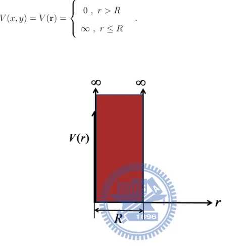
And the only assumption for the scattering potential (see Fig. 2.1) is that V (x, y) = V (r) =      0 , r > R ∞ , r ≤ R . (2.9)

Figure 2.1: Radial profile of ”hard” wall disk of our system.

The dispersion relation in Eq. (2.5) represents two parabolic bands Fig. 2.2 centered up k = −η(β1κ2)

2 . For states propagating with their momentum k making a angle ϕk with

respect to the ˆx axis Fig. 2.3 and for an energy E ≥ 0, there exit a degenerate states

which is ψin,+ = 1 √ 2    1 <    eik·r , (2.10) ψin,− = 1 √ 2    1 −<    eik0·r , (2.11)

where −→k = k [cos(ϕk)ˆx + sin(ϕk)ˆy] and

− →

k0 _{= k}0_[cos(ϕ

k)ˆx + sin(ϕk)ˆy] whom we can get

by solving ε = k2_{+ β}

1kκ2 = k02− β1k0κ2 .

The states ψin,+ represent plane wave states with helicity (η = +) whose spin states are

perpendicular to the momentum direction. The detail derivation of the eigenstates and eigenvalues is in the appendix.

Figure 2.2: Energy dispersion with helicity η for a linear-k Dresselhaus system ; the blue line correspond to η = + and the red line correspond to η = −. The dash line means that system has no spin-orbit coupling (β1 = 0) and Eq. (2.5) represents two parabolic bands

centered up k = −η(β1κ2)

2 .

A plane wave corresponding to an free electron propagating with the momentum vector

− →

k making a propagating angle ϕkwith ˆx axis, in accordance with Jacobi-Anger expansion

[30] which can be expanded as a linear superposition of the circular free waves

eik·r_{= e}ikr cos(ϕ−ϕk) ₌

∞

X

m=−∞

im_J

Figure 2.3: The plane wave of an incident electron wave with wave vector k making an angle ϕk with ˆx axis gets scattered by a scattering region defined by a Dresselhaus SOI

and a ”hard” wall disk.

Then the incident plane wave with momentum k and helicity (η = +) can be decom-posed as the following linear superposition:

ψin,+ = 1 √ 2 ∞ X m=−∞    i m_J m(kr)eim(ϕ−ϕk) (+<)im−1_J m−1(kr)ei(m−1)(ϕ−ϕk)    (2.13)

Since Bessel function Jm(kr) is a standing wave along the radial direction, for our

purpose, it is easily to express it in terms of two radial propagating waves, the Hankel functions, Jm(kr) = 1 2 £ H_m(1)(kr) + H_m(2)(kr)¤ , (2.14)

where the first kind and the second Hankel functions are defined as

Hm(1)(z) = Jm(z) + iYm(z) ;

Hm(2)(z) = Jm(z) − iYm(z) .

(2.15)

In the region where kr À 1 the radial propagating dependence of these Hankel functions become most apparent in their asymptotic form,

lim kr→∞H (1) m (kr) ∼ √1_kreikr ; lim kr→∞H (2) m (kr) ∼ √1_kre−ikr . (2.16)

For large r, Hm(1)(kr) goes like eikr

±

r, we can regard it as a circular waves propagating

radial outwards from the scattering center. In the same way, Hm(2)(kr) can be treated as

a circular waves propagating radial inwards from the scattering center.

To consider the scattering process for the cylindrical symmetric potential, we decom-pose Bessel function Jm(kr) (standing waves) as Hankel functions Hm(2)(kr) (incoming

waves) and Hm(1)(kr) (outgoing waves) so Eq. (2.13) become

ψin,+ = 1 2√2 ∞ X m=−∞    i mh_H(2) m (kr) + Hm(1)(kr) i eim(ϕ−ϕk) (+<)im−1h_H(2) m−1(kr) + Hm−1(1) (kr) i ei(m−1)(ϕ−ϕk)    (2.17) or = 1 2√2 ∞ X m=−∞ im    h Hm(2)(kr) + Hm(1)(kr) i eim(ϕ−ϕk) (−i<) h H_m−1(2) (kr) + H_m−1(1) (kr) i ei(m−1)(ϕ−ϕk)    (2.18) where < = −e−iϕk _.

helicity, the wave function is given by ψin,+ = 1 2√2 ∞ X m=−∞ im    h Hm(2)(kr) + Hm(1)(kr) i eim(ϕ) (i) h H_m−1(2) (kr) + H_m−1(1) (kr) i ei(m−1)(ϕ)    (2.19)

The cylindrical symmetry of the scattering potential cause waves to be coupled only with the same m . This essentially the conservation of the conservation of orbital angular momentum, which is true for a center potential but no SOI.

2.1.2

Cylindrical form representation of the eigenstates

In cylindrical coordinates, which are useful when we consider scattering from a localized , cylindrically symmetric potential, Hamiltonian can be written as

ˆ H =    −∇ 2 _−κ2_β 1ˆk+ −κ2_β 1ˆk− −∇2    (2.20) where ∇2 ₌ ∂2 ∂r2 + 1_r∂r∂ +_r12 ∂ 2 ∂ϕ2 and

ˆk±= ˆkx± iˆky = −ie±iϕ(

∂ ∂r ± i r ∂ ∂ϕ) . (2.21)

The raising and lowering operators ˆk± work on Bessel function through the the recurrence

relations ℘0 m(z) + mz℘m(z) = ℘m−1(z) ℘0 m(z) −mz℘m(z) = −℘m+1(z) (2.22)

where ℘ denotes, Bessel function, Neumann function and Hankel function that we can get a relation

The total Hamiltonian ˆH commutes with the z projection of the total angular momentum

ˆ

Jz = Lz+

1

2σz (2.24)

that allows one to representation eigenstate of Eq. (2.20) as

ψm =    Am(r)e imϕ Bm0(r)eim 0_ϕ    (2.25)

Am(r) and Bm0(r) are both radial dependent , so we can make A_m(r) = A0J_m(γr) and

Bm0(r) = B0J_m0(γr) (m0 = m − 1) where A0 and B0 are arbitrary constants.

ψm =    A 0_J m(γr)eimϕ B0_J m−1(γr)ei(m−1)ϕ    (2.26)

Substituting Eq. (2.23) into ˆHψm = εψm, one can obtain the following systems of radial

equations: ³ {−1 r ∂ ∂r(r ∂ ∂r) + m2 r2} − ³ ε + κ2_β 1iγB 0 A0 ´´ Jm(γr) = 0 , ³ {−1 r∂r∂ (r∂r∂) + (m−1)2 r2 } − ³ ε − κ2_β 1iγA 0 B0 ´´ Jm−1(γr) = 0 . (2.27)

The above equation must hold for the equation Eq. (2.28) due to the properties of Bessel function γ2 _{= ε + κ}2_β 1iγ B0 A0 = ε − κ 2_β 1iγ A0 B0 (2.28)

To simplify our calculation, we define R = B0

A0. After calculation, we can get energy

dispersion

and the ratio R

R = ηi (η = ±) . (2.30)

Consequently , the energy eigenstates of Hamiltonian with momentum γ, helicity η, and a ratio value < are

ψηm(r, ϕ) =

 

 Ωηm(γr)e

imϕ

(ηi)Ωη(m−1)(γr)ei(m−1)ϕ

 

 , (2.31)

where Ωη,m can be a Bessel function, a Neumann function and a Hankel function. Here

we choose Hankel functions as the eigenbasis to suit our boundary condition during the scattering process. The detail dervation of solving eigenequation is presented in appendix.

2.2

Cubic-k Dresselhaus SOI

2.2.1

Incident plane wave

The Hamiltonian for a 2DEG in the presence of the Dresselhaus SOI with a circular hard-wall disk at the origin can be expressed,

H = −∇2+ βkx(k2y− κ2)σx+ βky(κ2− kx2)σy+ V (

*

r) (2.32) where σj are the Pauli spin matrices and β is the Dresselhaus spin-orbit coupling constant

. In order to distinct the contribution from the linear-k and cubic-k Dresselhaus SOI, we change the Hamiltonian form Eq. (2.32) into Eq. (2.33).

H = −∇2− κ2β1(kxσx− kyσy) + β3(kxky2σx− kykx2σy) + V (

*

where β1 related to the linear-k Dresselhaus SOI and β3 related to the cubic-k Dresselhaus

SOI. The assumption for the scattering potential is same in the linear-k case (see Fig. 2.1). The eigenstates and correspond eigenvalues for the free-particle Hamiltonian (r ≥ R) with Dresselhaus spin-orbit coupling are given by

ψin,η(r, ϕ, ϕk) = eik·rχη , (2.34) ε = k2_{+ ηβ} 1k s κ4_{+ [} β3 2β1 k2_sin(2ϕ k)]2− β3 β1 k2_κ2_sin2_(2ϕ k) , (2.35) where χη(ϕk) = 1 √ 2    1 R    =√1 2    1 η<    , (2.36) tan(ϕk) = k_ky_x, R = η< , (2.37) and < = − v u u t κ2e−i(ϕk)+ 2ββ31ik 2_sin(2ϕk)ei(ϕk) κ2_ei(ϕk)− β3 2β1ik 2_sin(2ϕ k)e−i(ϕk) . (2.38)

where < denoting a ratio value which is function of incident angle and Dresselhaus SOI constant. The detail derivation of the eigenstates and eigenvalues shown in the appendix. The dispersion relation in Eq. (2.35) represents two helicity (η = ±) branches.

For states propagating with their momentum vectors making an angle ϕkwith respect

with the degenerate with the degenerate states are given by ψin,+ = eik·r 1 √ 2    1 <    , (2.39) ψin,− = eik 0_·r 1 √ 2    1 −<    , (2.40)

where −→k = k (cos(ϕk)ˆx + sin(ϕk)ˆy) and

− →

k0 _{= k}0_(cos(ϕ

k)ˆx + sin(ϕk)ˆy) which you can

obtain by solving ε = k2+ β1k s κ4_{+ [}β3 2β1 k2_sin(2ϕk)]2₋ β3 β1 k2_κ2_sin2_(2ϕ k) (2.41) and ε = k02− β1k0 s κ4 _{+ [}β3 2β1 k02_sin(2ϕ k)]2− β3 β1 k02_κ2_sin2_(2ϕ k) . (2.42)

The states Eq. (2.39) and Eq. (2.40) represent plane wave states with spin states shown in Eq. (2.36) being in the plane, perpendicular to the momentum direction. A plane wave corresponding to an free electron propagating with the momentum vector −→k making a

propagating angle ϕk with ˆx axis, in accordance with Jacobi-Anger expansion which can

be expanded as a linear superposition of the circular free waves

eikr_{= e}ikr cos(ϕ−ϕk) =

∞

X

m=−∞

im_J

m(kr)eim(ϕ−ϕk) . (2.43)

Eq. (2.41) can be decomposed as the following linear superposition: ψin,+ = eikr √ 2    1 <    = e ikr cos(ϕ−ϕk) √ 2    1 <    = √1 2     P m Jm(kr)eim(ϕ−ϕk) P m0 (<)Jm0(kr)eim 0_(ϕ−ϕ k)     (2.44)

And then we can deal with cubic Dresselhaus SOI case in the same way just like plane wave in a linear Dresselhaus system.

Considering the scattering process with the cylindrical symmetric potential , we decom-pose Bessel function Jm(kr) (standing waves) as Hankel functions Hm(2)(kr) (incoming

waves) and Hm(1)(kr) (outgoing waves) so Eq. (2.45) become

ψin,+ = 1 2√2 ∞ X m,m0_=−∞    i mh_H(2) m (kr) + Hm(1)(kr) i eim(ϕ−ϕk) (<)im0h H_m(2)0(kr) + H_m(1)0(kr) i eim0_(ϕ−ϕ k)    . (2.45)

2.2.2

Cylindrical form representation of the eigenstates

In polar coordinates, which are useful when we consider scattering from a localized, cylin-drically symmetric potential (hard − wall disk), Hamiltonian can be written as

ˆ H =    −∇ 2 _−κ2_β 1ˆk++β₄3(ˆk+2 − ˆk2−)ˆk− −κ2_β 1ˆk−− β₄3(ˆk+2 − ˆk2−)ˆk+ −∇2    (2.46) where ∇2 ₌ ∂2 ∂r2 + 1_r∂r∂ +_r12 ∂ 2 ∂ϕ2 and

ˆk±= ˆkx± iˆky = −ie±iϕ(

∂ ∂r ± i r ∂ ∂ϕ) (2.47)

potential, the eigenstates can be written as a two-component wave function. ψ(r, ϕ) =     P m Am(r)eimϕ P m0 Bm0(r)eim 0_ϕ     (2.48)

Since Am(r) and Bm0(r) both have radial-dependence, we assume that A_m(r) = A0_mJ_m(γr)

and Bm0(r) = B_m00J_m0(γr) . Then wavefunction become a two-component function which

is a linear superposition of Bessel functions

ψ(r, ϕ) =     P m A0 mJm(γr)eimϕ P m0 B0 m0J_m0(γr)eim 0_ϕ     (2.49) where A0

m and Bm00 are unknown constants which are determined by eigenequations. And

then we can deal with cubic-k Dresselhaus SOI case in the same way similar to plane wave in a linear-k Dresselhaus system.

ˆkν[Jm(γr)eimϕ] = iγνJm+ν(γr)ei(m+ν)ϕ (ν = ±) . (2.50)

Substituting Eq. (2.49) and Eq. (2.50) into equation ˆHψ = εψ, one can obtain the

fol-lowing radial equations:

{−1 r∂r∂(r∂r∂) + m 2 r2 − (ε + κ2β1γi B0 m−1 A0 m − i β3 4γ3 B 0 m−1 A0 m + i β3 4 γ3 B 0 m+3 A0 m )}Jm(γr) = 0, {−1 r∂r∂(r∂r∂) + m 2 r2 − (ε − κ2β1iγ A0 m+1 B0 m − i β3 4γ3 A 0 m−3 B0 m + i β3 4 γ3 A 0 m+1 B0 m )}Jm(γr) = 0. (2.51) By setting A0 m ∼ A0xm , Bm0 ∼ B0xm (2.52)

and using properties of Bessel functions, gives rise to Eq. (2.51) (ε + κ2_β 1γiB 0 A0x−1− i β3 4 γ3 B 0 A0x−1+ i β3 4γ3 B 0 A0x3) = (ε − κ2_β 1iγA 0 B0x − iβ₄3γ3 A 0 B0x−3+ iβ₄3γ3 A 0 B0x) = γ2 _. (2.53)

To simplify our calculations, we let R = B0_/A0_{. We also assume that R=e}iθ _{and x = e}iδ

are both phase vectors. As a result, we obtain two simple relations

ε + ei(θ+δ)_β 1γ(iκ2e−i2δ −β_β3₁γ 2 2 sin(2δ)) = ε − e−i(θ+δ)_β 1γ(iκ2ei2δ +β_β3₁γ 2 2 sin(2δ)) = γ2 (2.54)

between momentum γ and energy ε . From Eq. (2.54), the unknown values can be solved. The eigenstate is ψη(r, ϕ) =     P m

Jm(γr)eimϕeimδ

P m0 (η<)Jm0(γr)eim 0_ϕ eim0_δ     (2.55) where < = e−iδ v u u t− (iκ2ei2δ +ββ31 γ2 2 sin(2δ)) (iκ2_e−i2δ₋ β3 β1 γ2 2 sin(2δ)) (2.56) and eigenenergy is ε = γ2_{+ ηβ} 1γ s κ4_{+ (}β3 β1 γ2 2)2sin 2_{(2δ) − κ}2β3 β1 γ2_sin2_{(2δ) . (2.57)}

Here η = ± can be viewed as helicity + and helicity −. Consequently , the energy eigenstates of Hamiltonian Eq. (2.46) with momentum γ, a phase δ, helicity η, and a

ratio value < are ψη(r, ϕ) =     P m

Ωm(γr)eimϕeimδ

P m0 (η<)Ωm0(γr)eim 0_ϕ eim0_δ     (2.58)

where Ω can be a Bessel function, a Neumann function and a Hankel function. Here we choose Hankel functions as the eigenbasis to suit our boundary condition at infinity during the scattering process. The detail derivation of solving eigenequation is presented in Appendix.

2.3

Energy dispersion of Dresselhaus SOI system

In this section, we discuss the energy dispersion of Dresselhaus SOI system including linear and cubic k. For given energy dispersions from the Eq. (2.5) and Eq. (2.35), we find that the energy dispersion in cubic k DSOI system Eq. (2.35) which is dependent on the incident angle ϕk. As a result, we propose energy dispersion diagrams in different

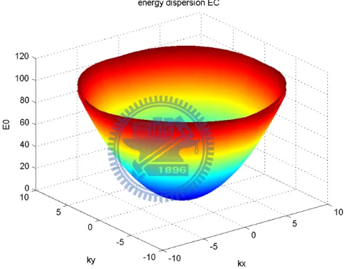
scales which are given by Fig. 2.4 and Fig. 2.5. On the other hand, the energy dispersion in linear k DSOI system

ε = k2± (βκ2)k

is like in the RSOI system

ε = k2_{± αk}

but the spin orbit couple strength in the later case is stronger ( α À ˜β = βκ2₎

βκ2

α =

¡

27eVA3¢(0.209nm )2

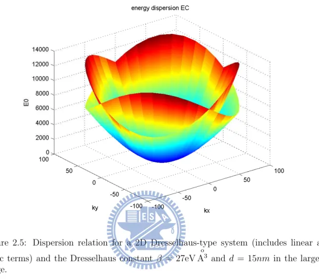
The twofold denervate branch (η = ±) is unapparent due to the small k contribution that we found from Fig. 2.4. In contrast, the degeneration is more apparent in Fig. 2.5 if k becomes larger gradually in the larger k range. In the specific incident plane angle Eq. (2.35) is reduced to Eq. (2.5). We can use the special cases to know what differential contribution from linear and cubic k although the cubic k contribution is smaller. At the same time, the DSOI linear k result can be compared with the RSOI result [16].

Figure 2.4: Dispersion relation for a 2D Dresselhaus-type system (includes linear and cubic terms) and the Dresselhaus constant β = 27eVAo3 _{and d = 15nm.}

Figure 2.5: Dispersion relation for a 2D Dresselhaus-type system (includes linear and cubic terms) and the Dresselhaus constant β = 27eVAo3 _{and d = 15nm in the larger k}

range.

On the other hand, we obtain three roots by solving the energy dispersion in cubic-k system Eq. (2.35) for a given energy ε and incident angle ϕk. For the example, the

incident angle ϕk is π₃ and the helicity is positive so that we can evaluate the roots of the

energy dispersion in Fig. 2.6.

The roots of the energy dispersion Eq. (2.35) where ϕk= π₃ and η = +. The right pattern

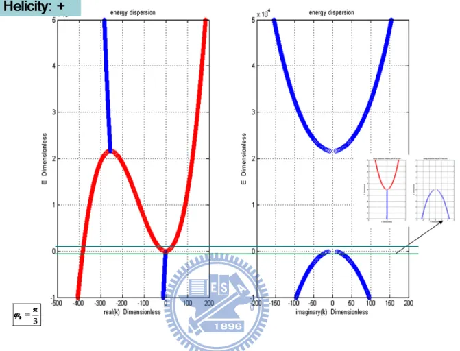
is the real part of k and the left pattern is the imagine part of k. In the central region of the real k and k imagine pattern show that the three roots in the region are all pure real values. Apparently, the momentum k we have to neglect is only the smallest one due to the corresponding much fast oscillation and then the others are exactly we must consider. By the way, the energy ε in the top and bottom regions of the real k and imagine k pattern are not the incident energy so that here we don’t discuss them. Similarly, if the energy

dispersion has negative helicity, we also can use the manner to obtain the momentums in the same way. The smaller pattern of Fig. 2.6 is the energy dispersion of the incident plane wave where the incident energy ε which we consider is located in the energy region. But just like the energy dispersion

ε = k2_{+ ηβ} 1k s κ4_{+ [} β3 2β1 k2_sin(2ϕ k)]2− β3 β1 k2_κ2_sin2_(2ϕ k)

we have derived before, the incident wave angle ϕk can determine the number of roots

of the energy dispersion. However, the roots of the energy dispersion in linear-k DSOI system Eq. (2.5) or in cubic-k DSOIsystermEq. (2.35) we need are both two roots.

Figure 2.6: The roots of the energy dispersion Eq. (2.35) where ϕk = π₃ and η = +.

The right pattern is the real part of k and the left pattern is the imagine part of k. In the central region of the real k and k imagine pattern show that the three roots in the region are all pure real values. Apparently, the momentum k we have to neglect is only the smallest one due to the corresponding much fast oscillation and then the others are exactly we must consider.

2.4

BIA in spin splitting in 2D systems

For two dimension systems,we can estimate the BIA-induced spin splitting. We obtain a spin splitting ∆ε(*k) = ±β1k s κ4_{+ [} β3 2β1 k2_sin(2ϕ k)]2− β3 β1 k2_κ2_sin2_(2ϕ k) (2.59)

to the origin shape (β1 = β3 = β) and Eq. (2.59) becomes ∆ε(k) = ±βk r κ4_{+ [}1 4k2− κ2]k2sin 2_(2ϕ k) (2.60a) ≈ ±β · κ2_k2₋ 1 2κ 3_sin2_(2ϕ k) + a ¡ k5¢ ¸ . (2.60b)

where*k = k cos(ϕk)ˆx + k sin(ϕk)ˆy. We have used κ to replace with the expectation value

hkzi of the wave vector along z-direction. For small

*

k the BIA spin splitting is linear in

*

k and independent of the direction of *k. For larger values of *k the BIA spin splitting

becomes anisotropic, with energy surfaces that have a fourfold rotational symmetry. Note also that for ϕk = 0

³_*

k k [100]´and ϕk = π₄

³_*

k k [110]´ , Eq. (2.60) is exact [2]. Within

our approach we thus have zero BIA spin splitting for ϕk = π₄ and k2 = 2κ2.

2.5

Connection between linear-k DSOI and ROSI

sys-tems

For a 2DEG system, linear-k DSOI Hamiltonian is like RSOI Hamiltonian. We can make a coordinate rotation about DSOI Hamiltonian

HD = β (σxkx− σyky) (2.61)

and then the rotated DSOI Hamiltonian to compare with RSOI Hamiltonian

HR= α(σxky − σykx) (2.62)

where α is the Rashba spin orbiting constant and β is the Dresselhaus spin orbiting constants. Suppose, for instance, the [x0_{, y}0_{] system is rotated by angle θ Fig. 2.7, relative}

system and [x, y] system in matrix notation:    x 0 y0    =    cos(θ) sin(θ) − sin(θ) cos(θ)       x y    . (2.63)

Figure 2.7: the [x0_{, y}0_{] system is rotated by angle θ, retaliative to the [x, y] system.}

In the same way, Dresselhaus type Hamiltonian in [x0_{, y}0_{] system is}

H0

D = β (kx0σ_x0 − k_y0σ_y0)

and then it is transformed into [x0_{, y}0_{] system after coordinate rotation. Similar to}

Eq. (2.63), we can use the same rotation matrix in momentum kx0(k_y0) and Pauli

ma-trix σx0(σ_x0). The detailed derivation of the coordinate rotation between linear-k DSOI

and RSOI Hamiltonians are shown in the appendix. After a coordinate rotation, the linear-k DSOI Hamiltonian in [x, y] system is given by

H0

We can chose a special rotating angle π

4 and then the corresponding rotated Hamiltonian

H0

D(

π

4) = HD = β (kxσy + kyσx) (2.65) is like ROI Hamiltonian Eq. (2.62) so that we can make a competition between them. It means that the propagating with their momentum k making a angle ϕk = π₄ with

respect to the ˆx axis in linear k Dresselhaus SOI system whose propagating process is

compellable. We can discuss the spin density or the probability density distribution in this case comparing the Rashba result.

Scattering from a cylindrically

symmetric potential in a Dresselhaus

SOI system

The main focus in this chapter is discussed the scattering process. We first present the spin dependent scattering calculation including cylindrical wave representations of the incoming wave and the outgoing wave and then for a given m these equations involving Hankel functions can be transformed into a m × m matrices result from independence of the angle. We can determine the unknown coefficients by solving this boundary condition problem.

In contrast, the scattering process in linear-k DSOI system can be solved analytically so that the total function and the spin density both have analytical forms. The spin density distribution is evaluated exactly and it is helpful to analyze the cubic-k DSOI case. For a given total wave function, spin density will be studies. Finally, we drive particle continuity equation in Dresselhaus SOI Hamiltonian to find the particle current.

3.1

Cubic-k Dresselhaus SOI

3.1.1

Coupled cylindrical wave representations of the incoming

wave

First, we choose the propagating direction of the incident plane wave along ˆx-direction

with the angle ϕk respecting to the ˆx axis in Drsselhaus-type SOI system. Then, in

cylin-drical coordinate, incident plane wave with the incident energy ε, a ratio <, momentum

γ and helicity η = + can be expansion of partial waves

ψincoming = 1 2√2 ∞ X m,m0_=−∞    i m_H(2) m (γr)eim(ϕ−ϕk) <incim 0 H_m(2)0(γr)eim 0_(ϕ−ϕ k)    . (3.1)

For the scattering process in the Dresselhaus-type system we can take ψ as a eigenbasis

ψ = A     P m

Jm(γr)eimϕeimδ

P m0 (η<)Jm0(γr)eim 0_ϕ eim0_δ     (3.2) where < = e−iδ v u u t− (iκ2ei2δ +ββ31 γ2 2 sin(2δ)) (iκ2_e−i2δ₋ β3 β1 γ2 2 sin(2δ)) (3.3) , A is a unknown constant and

ε = γ2_{+ ηβ} 1γ s κ4_{+ (}β3 β1 γ2 2)2sin 2_{(2δ) − κ}2β3 β1 γ2_sin2_{(2δ). (3.4)}

due to the central cylindrical symmetric potential.

The total wave function outside the scattering region (r > R) has the form

where ψincoming = c    g1(γ, r, δ) g2(γ, r, δ)    (3.6) and ψoutgoing = Z _2π 0 dδa(δ)    f1(γ, r, δ) f2(γ, r, δ)    + Z _2π 0 dδ0b(δ0)    f1(γ 0_{, r, δ}0₎ f2(γ0, r, δ0)    . (3.7)

(postive helicity : γ , δ negative helicity : γ0_{, δ}0₎

Here f1(f2) are the first kind Hankel functions and g1(g2) are the second kind Hankel

functions. From Eq. (3.5) to Eq. (3.7), it can show that if an incident wave has a specific helicity ψin,+, no incoming cylindrical wave with negative helicity and nonzero coefficient

b(δ0_{) lead to outgoing waves with flipped helicity (outgoing wave must have both η = ±).}

For a given incident plane wave Eq. (3.1), we look at the incoming part that the all coefficients in Eq. (3.6) can be determined and use <incto replace with < where <inc is a

function of ϕk in order to avoid to confuse the incoming wave with the outgoing wave.

ψincoming = 1 2√2 ∞ X m,m0_=−∞    i m_H(2) m (γr)eim(ϕ−ϕk) <incim 0 H_m(2)0(γr)eim 0_(ϕ−ϕ k)    (3.8) ε = γ2_{+ β} 1γ s κ4_{+ [} β3 2β1 γ2_sin(2ϕ k)]2 − β3 β1 γ2_κ2_sin2_(2ϕ k) (3.9) <inc = − v u u t κ2e−i(ϕk)+ 2ββ31iγ 2_sin(2ϕ k)ei(ϕk) κ2_ei(ϕk)− β3 2β1iγ 2_sin(2ϕ k)e−i(ϕk) (3.10) Boundary conditions will be established in the later section for the solving of unknown coefficients of outgoing wave Eq. (3.7). And we simplify the outgoing wave part in the next section.

3.1.2

Coupled cylindrical wave representations of the outgoing

wave

The continuous integrationR₀2πdδ in Eq. (3.7) can be treated as the discrete summation

N

P

i=1

∆δ in representation of a matrix form to and then use it to solve the boundary problem in the numerical method. Here δ describes that the integration range of δ from 0 to 2π is divided into N pieces and each piece ∆δ = 2π/N. The summation is more close to the integration if N is larger enough. In the later section, we can determine N through the numerical result of the spin density and the probability of the total wave function. The integration approximation is estimated by

Z _2π 0 dδ → N X i=1 ∆δ and R₀2πdδ0 _→ PN i=1 ∆δ0 _(3.11)

The outgoing wave part of the total wave function Eq. (3.7) can be regarded as the discrete form ψoutgoing = N X n=1 ∆δa(δn)    f1(γn, r, δn) f2(γn, r, δn)    + N X n=1 ∆δ0_b(δ n)    f1(γ 0 n, r, δn0) f2(γn0, r, δn0)    (3.12) where ∆δ = 2π

N = ∆δ0 and δn = n∆δ = n∆δ0 = δ0n. The unknown constants a(δn) and

b(δn) are function of δn and then δn is the Nth piece of the angle δ. Substituting the

eigenbasis Eq. (3.2) into the Eq. (3.12), we have the outgoing wave function in the dis-crete form ψoutgoing = N P n=1 ∆δa(δn)     ∞ P m=−∞ Hm(1)(γnr)eim(ϕ+δn) (<n) ∞ P m0_=−∞ H_m(1)0(γnr)eim 0_(ϕ+δ n)     + PN n=1 ∆δ0_b(δ0 n)     ∞ P m=−∞ Hm(1)(γ_n0r)eim(ϕ+δ 0 n) (<0 n) ∞ P m0_=−∞ H_m(1)0(γ_n0r)eim 0_(ϕ+δ0 n)     (3.13)

The equation shows that consider a incident plane wave with positive helicity after scat-tering by central symmetric potential ( hard wall disk) whose incoming wave part is the same as before scattering but the outgoing wave part including both positive and negative helicity lead to spin flipping. For a reference, if the incident wave has only negative he-licity, then the helicity of the incoming wave part is still negative. At the same time, the rules of γ and γ0_{, as well as the probability amplitudes a(δ) and b(δ}0_{) must be interchanged.}

We can easily deduce the outgoing wave function into the convenient form with the representation am(δn) = am and bm0(δ_n) = b_m0 and then it becomes

ψoutgoing = N X n=1 ∆δ     ∞ P m=−∞

[anHm(1)(γnr)eim(ϕ+δn)+ bnHm(1)(γn0r)eim(ϕ+δn)] ∞ P m0_=−∞ [an(<n)Hm(1)0(γ_nr)eim 0_(ϕ+δ n)+ b n(<0n)H (1) m0(γ_n0r)eim 0_(ϕ+δ n)]     (3.14) Here the correspond energy dispersion and the ratio are

ε = γ2 n+ β1γn s κ4_{+ (}β3 β1 γ2 n 2 )2sin 2_(2δ n) − κ2 β3 β1 γ2 nsin2(2δn) , (3.15) <n = e−iδn v u u t− (iκ2ei2δn+ ββ31 γ2 n 2 sin(2δn)) (iκ2_e−i2δn− β3 β1 γ2 n 2 sin(2δn)) (3.16) and ε = (γ_n0)2− β1γn0 s κ4_{+ (}β3 β1 (γ0 n)2 2 )2sin 2_(2δ n) − κ2β3 β1 (γ0 n)2sin2(2δn) , (3.17) <0_n = −e−iδn v u u t− (iκ2ei2δn+ ββ31 (γ0 n)2 2 sin(2δn)) (iκ2_e−i2δn− β3 β1 (γ0 n)2 2 sin(2δn)) (3.18)

; Eq. (3.15) and Eq. (3.16) corresponding to helicity η = + , while Eq. (3.17) and Eq. (3.18) correspond to η = −. In the case of helicity η = +, for a given energy ε, momentum γn can be get from the energy dispersion in each δn. And then if momentum

is known, we also obtain the correspond ratio <nby solving the equation which is function

of η and δnEq. (3.16). The negative helicity case is the same as the negative helicity case ,

so all parameters is known for a given energy expect for the probability anand bnwhich we

can determine by the boundary condition. After detailed calculation process in section 3.1 and this section, from the incoming wave part in Eq. (3.8) and the outgoing wave part in Eq. (3.14), the total wave function with the incident angle ϕkoutside the disk Eq. (3.5)

is given by ψtotal(r, ϕ, ϕk) =             N P n=1 ∞ P m=−∞

∆δ[anHm(1)(γnr)eim(ϕ+δn)+ bnHm(1)(γ0nr)eim(ϕ+δn)]

+ 1 2√2 ∞ P m=−∞ im_H(2) m (γr)eim(ϕ−ϕk) N P n=1 ∞ P m0_=−∞ ∆δ[an(<n)Hm(1)0(γnr)eim 0_(ϕ+δ n)+ b n(<0n)H (1) m0(γ_n0r)eim 0_(ϕ+δ n)] + 1 2√2 ∞ P m0_=−∞ (<inc)im 0 H_m(2)0(γr)eim 0_(ϕ−ϕ k)             (3.19) The total wave function ϕk outside the scattering region (r ≥ R) for a given incident

angle must be zero which is independent of the angle ϕ at r = R due to the boundary condition of the cental symmetric potential ( ”hard ” wall disk).

ψtotal(R, ϕ, ϕk) =             N P n=1 ∞ P m=−∞

∆δ[anHm(1)(γnR)eim(ϕ+δn)+ bnHm(1)(γ_n0R)eim(ϕ+δn)]

+ 1 2√2 ∞ P m=−∞ im_H(2) m (γR)eim(ϕ−ϕk) N P n=1 ∞ P m0_=−∞ ∆δ[an(<n)H_m(1)0(γnR)eim 0_(ϕ+δn) + bn(<0n)Hm(1)0(γ_n0R)eim 0_(ϕ+δn) ] + 1 2√2 ∞ P m0_=−∞ (<inc)im 0 H_m(2)0(γR)eim 0_(ϕ−ϕ k)             = 0

(3.20) In Eq. (3.20) the summation P∞

m=−∞

we can define a finite range from −m to m to represent an infinite range just like Eq. (3.11) . At the same time, we make N in Eq. (3.11) equal 2M + 1 so that the first low of the total wave function is given by

M X m=−M Ã_{2M +1} X n=1 ∆δeim(ϕ+δn)_[a nfmn+ bnfmn0 ] + gmeim(ϕ−ϕk) ! (3.21) where fmn = Hm(1)(γnR) , fmn0 = H (1) m (γ_n0R) and gm = i m 2√2H (2) m (γR) .

And each piece ∆δ is equal to 2π

2M +1 corresponding δn = n∆δ = n2M +12π . In the same way,

the second low has the similar form

M X m0_=−M Ã_{2M +1} X n=1 ∆δeim0_(ϕ+δ n)_[a n(<n)fm0_n+ b_n(<0_n)f_m0 0_n] + (<_inc)g_m0eim 0_(ϕ−ϕ k) ! (3.22) where eiθn_f m0_n= (<_n)H_m(1)0(γ_nR) , eiθ 0 nf0 m0_n= (<0_n)H_m(1)0(γ_n0R) and g_m0 = i m0 2√2H (2) m0(γR) . Then

the total wave functions on the bound (r = R) reduce to a simply form as following

ψtotal(R, ϕ, ϕk) =     M P m=−M µ 2M +1_P n=1 ∆δeim(ϕ+δn)_[a nfmn+ bnfmn0 ] + gmeim(ϕ−ϕk) ¶ M P m0_=−M µ_{2M +1} P n=1 ∆δeim0_(ϕ+δ n)[a n(<n)fm0_n+ b_n(<0_n)f_m0 0_n] + (<_inc)g_m0eim 0_(ϕ−ϕ k) ¶     = 0 . (3.23) We use the orthogonal relation on the summations of the two component matrix since the ”hard” wall boundary is ϕ independent. Taking into the orthogonal relation on ϕ, the first low Eq. (3.21) have no ϕ dependence, we have

2M +1_X n=1 ³ eim00_δ n_[f m00_na_n+ f_m0 00_nb_n] ´ = − 1 ∆δGm00 (3.24)

where Gm00 = g_m00eim 00_(−ϕ

k)and we can do the same orthogonality on Eq. (3.22). Eq. (3.23)

can be transformed into a big matrix which is given by    F11 F12 F21 F22       A B    =    G G0    (3.25) where F11=       e−iM δ1f −M 1 . . . e−iM δ2M +1f−M (2M +1) ... . .. ... eiM δ1f M 1 · · · eiM δ2M +1fM (2M +1)       , (3.26) F12=       e−iM δ1f0 −M 1 . . . e−iM δ2M +1f−M (2M +1)0 ... . .. ... eiM δ2M +1f0 M 1 · · · eiM δ2M +1fM (2M +1)0       , (3.27) F21=       e−iM δ1(< 1)f−M 1 . . . e−iM δ2M +1(<2M +1)f−M (2M +1) ... . .. ... eiM δ1(< 1)fM 1 · · · eiM δ2M +1(<2M +1)fM (2M +1)       , (3.28) and F22=       e−iM δ1(<0 1)f−M 10 . . . e−iM δ2M +1(<02M +1)f−M (2M +1)0 ... . .. ... eiM δ2M +1(<0 1)fM 10 · · · eiM δ2M +1(<02M +1)fM (2M +1)0       . (3.29)

The unknown matrix elements

A =       a−M 1 ... aM 2M +1       (3.30)

and B =       b−M 1 ... bM 2M +1       (3.31)

can be solved in the numerical method for a given

G =       G−M ... GM       and G0 ₌       (<inc)G−M ... (<inc)GM       .

Appendix gives the detailed derivation of the matrix in Dresselhaus-type SOI system. The numerical result of Eq. (3.30) and Eq. (3.31) can be used to obtain the total wave function Eq. (3.23) so that the spin density is determined. Also, we can observe the spin density pattern via the incident angle ϕk in the summation.

3.2

Linear-k Dresselhaus SOI

3.2.1

Coupled cylindrical wave representations

From the section 2.2, we know that the direction of the propagating of the incident plane wave along the ˆx axis in linear-k Dresselhaus SOI system. Then, in cylindrical coordinate,

partial waves ψin,+ = ∞ X m=−∞ im 2√2    h Hm(2)(γr) + Hm(1)(γr) i eim(ϕ) (i) h H_m−1(2) (γr) + H_m−1(1) (γr) i ei(m−1)(ϕ)    . (3.32)

and m is the total angular momentum which is conserved during the scattering. The energy eigenstate of the linear-k DSOI Hamiltonian can be written as

ψ_m =          eimϕh_a mHm(1)(γr) + cmHm(1)(γ0r) + i m 2√2H (2) m (γr) i ei(m−1)ϕh_ia mHm−1(1) (γr) − cmiHm−1(1) (γ0r) + i m 2√2(i)H (2) m−1(γr) i          (3.33) where ε = γ2_{+ β} 1κ2γ = γ02− β1κ2γ0.

The first and third terms have positive helicity while the second terms have the negative helicity. Here H(1,2)_{refers to the Hankel functions of the first and second kind respectively,}

and H(1)_[H(2)_{] is an outgoing (incoming) cylindrical wave. The most general eigenstates}

is a superposition of ψm, where the coefficients am and cm are determined by boundary

conditions. On the other hand, dm is determined by the initial condition in Eq. (3.32),

so we can obtain dm = i

m

2√2. It means that the incident plane wave has η = +, then

by comparing Eq. (3.33); the incoming wave (the second kind of the Hankel function) only has positive helicity, so dm can be obtained. For a ”hard ” wall boundary (i.e.

ψ_m = 0 at r = R), the coefficient can be given by

am = − i m 2√2 Hm(1)(˜γ0)Hm−1(2) (˜γ)+H (2) m (˜γ)Hm−1(1) (˜γ0) Hm(1)(˜γ)Hm−1(1) (˜γ0)+H (1) m (˜γ0)Hm−1(1) (˜γ) , cm = i m 2√2 Hm(1)(˜γ)H(2)m−1(˜γ)−H (2) m(˜γ)Hm−1(1) (˜γ) Hm(1)(˜γ)H(1)m−1(˜γ0)+H (1) m(˜γ0)Hm−1(1) (˜γ) , (3.34)

where we define ˜γ ≡ γR and ˜γ0 _{≡ γ}0_{R . The total wave function is the summation of}

partial wave can be represented by

ψtotal =

X

m

ψm . (3.35)

The Rashba scattering model has been investigated in [16].

To produce the recursion relation of the total wave function, we simplify Eq. (3.33)

ψ_m =    e imϕ_A +m ei(m−1)ϕ_B +m    (3.36) where A+m = amHm(1)(γr) + cmHm(1)(γ0r) + Hm(2)(γr) B+m = iamHm−1(1) (γr) − cmiHm−1(1) (γ0r) + iH (2) m−1(γr) . (3.37)

We would obtain the relation of the coefficients

a−m+1 = i−2m+1am c−m+1 = −i−2m+1cm (3.38) and B+,−m+1 = (−1)miA+,m B∗ +,−m+1 = −(−1)miA∗+,m . (3.39)

from the coefficient Eq. (3.34) if we have the properties of Hankel functions.

H−m(z) = (−1)mHm(z) (3.40)

The spin density of the total wave function in Eq. (3.32) for linear-k DSOI system can be obtained in analytical form if we use the recursion relation in Eq. (3.39). However,

the cubic-k DSOI system has to be solved in numerical method. The analytical form of the spin density is much more powerful which can be compared with the Rashba SOI scattering case [28].

3.3

Scattering of the scattering state

The scattering of the scattering state is composed of two kinds of outgoing waves (helicity

η = ± ) which resulted from scattering upon a hard disk. We change the helicity of

incident plane wave which is from the previous case and then the scattering process is analogical. But the quantity of spin density is slightly different.

3.4

Spin density of the scattering state

In the section we focus on the spin density of the scattering state both in linear-k DSOI and cubic-k DSOI systems. The spin density distribution is very important since we observe the polarization around the disk from the distribution. Moreover, for a given incident angle ϕk, we can obtain a spin density distribution. For the specific incident

angle, it can be compared with the one in the Rashba SOI system. At the same time, it is important is to know the cubic-k contribution by comparing the in linear-k DSOI with cubic-k DSOI systems. And then from the energy dispersion in cubic-k DSOI systems which was derived in section 2.2, we know that the scattering process is the same due to the same energy dispersion when the incident angle ϕk is equal to 2nπ (n is integer). In

contrast, at the other incident angle, the cubic-k SOI contribution is considerable. Here we must use the numerical method to deal with the spin density in cubic-k DSOI system, but the spin density can be obtained analytically in linear-k DSOI system.

The spin density on linear-k DSOI can be evaluated lightly since the total wave func-tion can be expressed in analytical form Eq. (3.33). By the definifunc-tion, the spin density