狀態相依跳躍風險與美式選擇權評價：黃金期貨市場之實證研究 - 政大學術集成

全文

(1)國立政治大學金融學系博士學位論文. 指導教授：廖四郎博士. 狀態相依跳躍風險與美式選擇權評價：政治. 大. 立黃金期貨市場之實證研究. ‧ 國. 學 ‧. State-Dependent Jump Risks and American Option Pricing:. Nat. n. al. er. io. sit. y. An Empirical Study of the Gold Futures Market. Ch. engchi. i n U. v. 研究生：連育民撰. 中華民國一百零三年六月.

(2) State-Dependent Jump Risks and American Option Pricing: An Empirical Study of the Gold Futures Market. 立. 政 by 治大 Yu-Min Lian. ‧. ‧ 國. 學. Nat. y. Supervisor. n. er. io. al. sit. Szu-Lang Liao. Ch. engchi. i n U. v. Department of Money and Banking National Chengchi University Taipei, Taiwan 114 R.O.C. June 2014.

(3) 中文摘要本文實證探討黃金期貨報酬率的特性並在標的黃金期貨價格遵循狀態轉換跳躍擴散過程時實現美式選擇權之評價。在這樣的動態過程下，跳躍事件被一個複合普瓦松過程與對數常態跳躍振幅所描述，以及狀態轉換到達強度是由一個其狀態代表經濟狀態的隱藏馬可夫鏈所捕捉。考量不同的跳躍風險假設，我們使用 Merton 測度與 Esscher 轉換推導出在一個不完全市場設定下的風險中立黃金期貨. 治政價格動態過程。為了達到所需的精確度，最小平方蒙地卡羅法被用來近似美式黃大立 ‧ 國. 學. 金期貨選擇權的價值。基於實際市場資料，我們提供實證與數值結果來說明這個動態模型的優點。. ‧. Nat. io. sit. y. 關鍵詞：美式黃金期貨選擇權、狀態轉換跳躍擴散過程、Merton 測度、Esscher. n. al. er. 轉換、最小平方蒙地卡羅法. Ch. engchi. I. i n U. v.

(4) Abstract. This dissertation empirically investigates the characteristics of gold futures returns and achieves the valuation of American-style options when the underlying gold futures price follows a regime-switching jump-diffusion process. Under such dynamics, the jump events are described as a compound Poisson process with a log-normal jump amplitude, and the regime-switching arrival intensity is captured by. 治政 a hidden Markov chain whose states represent the大 economic states. Considering the 立 ‧ 國. 學. different jump risk assumptions, we use the Merton measure and Esscher transform to derive risk-neutral gold futures price dynamics under an incomplete market setting.. ‧. To achieve a desired accuracy level, the least-squares Monte Carlo method is used to. sit. y. Nat. io. n. al. er. approximate the values of American gold futures options. Our empirical and. i n U. v. numerical results based on actual market data are provided to illustrate the advantages of this dynamic model.. Ch. engchi. Keywords: American gold futures option; Regime-switching jump-diffusion process; Merton measure; Esscher transform; Least-squares Monte Carlo method. II.

(5) Acknowledgements. First and foremost, I would like to thank my my supervisor Prof. Dr. Szu-Lang Liao who introduced me to the field of financial engeering, gave me valuable advice and support and who created the ideal environment for productive research at the Department of Money and Banking in National Chengchi University. Amongst the many people who gave me opportunity to discuss my ideas and provided valuable. 治政 feedback, I would like to thank particularly Dr. Mi-Hsiu 大 Chiang, Dr. Shih-Kuei Lin, 立 ‧ 國. 學. Dr. Chao-Chun Chen, Dr. Jui-Jane Chang, and my fellow students. I would also like to thank the participants at the various conferences and seminars where I presented. ‧. my work for their questions, comments and suggestions. At last, but not least, I. sit. y. Nat. io. n. al. er. express my thanks to my family for their support, particularly my parents for being. i n U. v. there for me at all times during my education and beyond.. Ch. engchi. III.

(6) Contents 中文摘要........................................................................................................................ I. Abstract ......................................................................................................................... II. Acknowledgements ...................................................................................................... III. Contents .......................................................................................................................IV. 政治大. List of Tables ................................................................................................................VI. 立. ‧ 國. 學. List of Figures ............................................................................................................ VII. ‧. 1. Introduction ................................................................................................................ 1. y. Nat. n. al. er. io. sit. 2. Model Framework and Pricing Method ..................................................................... 9. i n U. v. 2.1 Markov-modulated Poisson process ........................................................ 9. Ch. engchi. 2.2 Gold futures price modeling .................................................................. 11. 2.3 Least-squares Monte Carlo approach..................................................... 12. 3. Valuation of American Gold Futures Options in a Markov Regime-Switching Jump-Diffusion Economy ....................................................................................... 15. 3.1 Merton measure for the Markov regime-switching jump-diffusion process .................................................................................................. 16 IV.

(7) 3.2 Esscher transform for the Markov regime-switching jump-diffusion process .................................................................................................. 18. 3.3 Valuing American gold futures options.................................................. 22. 4. Empirical Analyses and Numerical Illustrations...................................................... 24. 4.1 Empirical results .................................................................................... 24. 4.2 Pricing performance ............................................................................... 34. 立. 政治大. 5. Conclusions and Future Extensions ......................................................................... 37. ‧ 國. 學. References .................................................................................................................... 39. ‧. Appendix A: Distributional properties of RSJM under Q M ....................................... 44. io. sit. y. Nat. n. al. er. Appendix B: Solving the Esscher parameters .............................................................. 47. Ch. engchi. i n U. v. Appendix C: Distributional properties of RSJM under Qθ ....................................... 49. V. m.

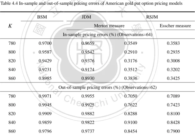
(8) List of Tables 4.1 Descriptive statistics of the gold futures returns .................................................... 25. 4.2 Estimated results of continuous-time models ........................................................ 30. 4.3 Distributional statistics for data and continuous-time models ............................... 31. 4.4 In-sample and out-of-sample pricing errors of American gold put option pricing. 政治大. models ................................................................................................................... 36. 立. ‧. ‧ 國. 學. n. er. io. sit. y. Nat. al. Ch. engchi. VI. i n U. v.

(9) List of Figures 1.1 Time series (top panel) and logarithmic returns (bottom panel) of daily gold futures prices ........................................................................................................... 3. 4.1 Graph of (a) gold futures prices, (b) logarithmic returns, (c) State probability, and (d) Jump probability.............................................................................................. 32. 4.2 Model autocorrelation of the squared logarithmic returns ..................................... 33. 立. 政治大. ‧. ‧ 國. 學. n. er. io. sit. y. Nat. al. Ch. engchi. VII. i n U. v.

(10) Chapter 1 Introduction Gold is a precious metal, which in recent years is considered to be an investment tool alternative to equity and bond markets. It provides similar functions as money in that it acts as a preserver of wealth, a medium of exchange and a unit of value. Unlike other commodities, gold is a special asset with renewable, relatively transportable,. 治政 universally acceptable and easily authenticated. The 大 unique and diverse drivers of 立 ‧ 國. 學. gold price behavior not highly correlate with changes in other financial assets. As a consequence, this precious metal can contribute in a saving role by acting as a type of. ‧. insurance against extreme movements and jumps in the value of traditional assets. sit. y. Nat. io. n. al. er. during times of economic and market stress (Capie et al., 2005; Baur and Lucey, 2010;. i n U. v. Baur and McDermott, 2010; Reboredo, 2013; Zagaglia and Marzo, 2013). Gold is a. Ch. engchi. liquid asset, continuously quoted on spot and futures markets and easy to trade. In addition to Beckers (1984) and Ball et al. (1985) empirically investigate the gold options market under the Black–Scholes framework, others, for instance, Ogden et al. (1990) study gold spot and futures options. It is well known that the presence of jumps in the underlying asset price can have significant implications on pricing derivatives, but these aforementioned papers do not address such jump phenomena.. 1.

(11) The increasing number of jump events, especially after the subprime financial crisis of 2008, has created large fluctuations in the gold futures prices and related derivatives (e.g., American gold futures options). For the market development, it is crucial in capturing the dynamic jump process appropriately and evaluate American gold futures options corresponding to the changing prices of gold futures.. Most exchange-traded option contracts are American style and therefore, many. 治政 numerical methods have been presented attempting 大to evaluate American options, 立 ‧ 國. 學. including the lattice (Cox et al., 1979), finite difference (Brennan and Schwartz, 1977; Hull and White, 1990), and Monte Carlo simulation methods (Boyle et al., 1997).. ‧. Increasing the number of steps comes at the cost of exponential growth in the size of. sit. y. Nat. io. n. al. er. the lattice pricing methods. Longstaff and Schwartz (2001) propose an algorithm for. i n U. v. pricing American options called least-squares Monte Carlo (LSM) approach. This. Ch. engchi. technique proceeds by simulating forward paths using the Monte Carlo simulation, and then performs backward iterations by applying least-squares approximation of the continuation function over a collection of basic functions. This algorithm is simple to implement within existing Monte Carlo frameworks, and has the additional advantages that the continuation functions are constructed explicitly and it is easy to calibrate to existing market prices. Therefore, we adopt this approach to evaluate. 2.

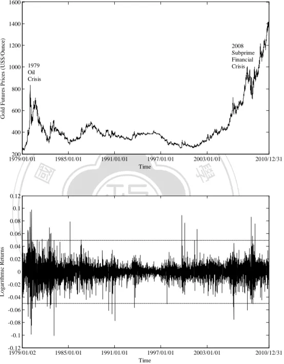
(12) American gold futures options.. 1600. 1200. 1000. 2008 Subprime Financial Crisis. 1979 Oil Crisis. 800. 600. 400. 立. 200 1979/01/01. ‧ 國. 0.02. y. al. n. 0. io. Logarithmic Returns. 0.04. Nat. 0.06. 2010/12/31. sit. 0.08. 2003/01/01. 1997/01/01 Time. ‧. 0.1. 1991/01/01. 學. 0.12. 1985/01/01. 政治大. er. Gold Futures Prices (US$/Ounce). 1400. -0.02 -0.04. Ch. engchi. i n U. v. -0.06 -0.08 -0.1 -0.12 1979/01/02. 1985/01/01. 1991/01/01. 1997/01/01 Time. 2003/01/01. 2010/12/31. Figure 1.1 Time series (top panel) and logarithmic returns (bottom panel) of daily gold futures prices Note that the dotted lines in the bottom panel denote the gold futures returns over ±5% in magnitude are jumps. The gold futures data is the one month forward contract attained from the continuous futures series from Datastream with switchovers at the first day of a new month. The futures contracts are the daily CMX-Gold-100-Oz.. 3.

(13) The top panel of Figure 1.1 draws some significant price jumps of gold futures in the daily data. 1 In particular, it shows that there are larger jumps (returns) in several time periods. In the oil crisis of 1979 and subprime financial crisis of 2008, for example, gold futures prices had larger jumps. The empirical data have revealed that the geometric Brownian motion (GBM) is not completely consistent with the reality, that is, the jumps do exist in the gold futures price realizations. Hence, incorporating. 政治大. sudden random shocks into a dynamic model is necessary and significant (Carr et al.,. 立. 2002; Eraker et al., 2003; Eraker, 2004; Maheu and McCurdy, 2004). In line with the. ‧ 國. 學. changing gold futures returns in the bottom panel of Figure 1.1, we could identify two. ‧. regimes of the gold futures market. The first state is defined as the relatively. y. Nat. io. sit. low-volatility regime and can be viewed as the ordinary state. The second state is. er. defined as the relatively high-volatility regime and can be regarded as the volatile. al. n. v i n C hthat, in the gold futures state. In addition, we also find e n g c h i U market, the bottom panel of Figure 1.1 exhibits different arrival rates of jump events in different time periods. It is an empirical fact that there exists the so-called jump and volatility clustering in the logarithmic return series of gold futures prices caused by a period of time of high (low) arrival rates tend to be followed by a period of time of continued high (low) arrival rates. Nevertheless, the existing jump-diffusion processes, such as in Merton (1976),. 1. The empirical data are from Datastream and cover the period from 01/01/1979 to 12/31/2010. 4.

(14) Amin (1993), and Kou (2002), are unable to address the phenomenon of volatility clustering. Duan et al. (2006) evaluate options when there are jumps in the pricing kernel and correlated jumps in asset prices and volatilities. The models capture leptokurtosis and volatility clustering but do not show the regime-switching phenomenon. Chan and Maheu (2002) propose a time-varying Poisson jump model to describe the jump dynamics of the stock prices in the discrete time circumstance. In. 政治大. the light of our empirical observations in Figure 1.1 with economic intuition, the. 立. change of gold futures prices represents that the economy stays in each state for a. ‧ 國. 學. period of time and then transitions to the other, as well as the jump intensity changes. ‧. over time according to the different regimes of the economy.. sit. y. Nat. io. n. al. er. In order to incorporate both unanticipated jump events and regime-switching. i n U. v. arrival rates in the oscillating gold futures market simultaneously, we model the gold. Ch. engchi. futures price dynamics using a regime-switching jump-diffusion model (RSJM) proposed by Chang et al. (2013). Under such a model, the jump events are described as a compound Poisson process with the log-normal jump amplitude setting applied by Merton (1976), and the regime-switching arrival intensity is governed by a continuous-time finite-state Markov chain. The states of the Markov chain can be interpreted as the hidden states of an economy. The regime-switching models are used. 5.

(15) to describe the asset price dynamics and are applied for option pricing. Elliott et al. (2007) investigate the option prices under a generalized Markov regime-switching jump-diffusion economy for the use of the Esscher transform employed by Elliott et al. (2005) and Elliott and Osakwe (2006) for valuing options under a regime-switching environment. Elliott and Siu (2011) incorporate structural changes in economic conditions in asset price dynamics and American option valuation. None of these. 政治大. discussions provide the empirical tests for the observed features and model fit of their. 立. dynamic processes. In this dissertation, we demonstrate that the dynamic model. ‧ 國. 學. describes the existence of jump events, leptokurtosis, asymmetry, and volatility. ‧. clustering for the gold futures returns, and illustrate the presence of regime-switching. y. Nat. n. al. er. io. models.. sit. arrival rates and jump clustering, and verify the superior empirical fit over competing. Ch. engchi. i n U. v. The market is incomplete in such a Markov regime-switching jump-diffusion economy, and we therefore need to select a pricing kernel for option valuation. Previous researches empirically illustrate that gold is either a zero or negative beta asset (McCown and Zimmerman, 2006; McCown and Zimmerman, 2007; Baur and Lucey, 2010; Baur and McDermott, 2010). This means that, under the CAPM assumptions, the jump component of the gold futures returns shows non-systematic or. 6.

(16) systematic risk. Thus, we make use of two specific approaches for choosing the martingale pricing measure to derive the risk-neutral gold futures price dynamics. First, we assume that the jump component of the gold futures returns presents non-systematic and diversifiable risk, that is, under the assumption that the jump risk is not priced, as in Merton (1976). Second, we relax this assumption to allow for the jump risk, regarding which as systematic and non-diversifiable. Then, the Esscher. 政治大. transform technique developed by Gerber and Shiu (1994, 1996) is considered to. 立. determine a risk-neutral pricing measure. After determining such martingale dynamics. ‧ 國. 學. of the gold futures prices, we use the LSM algorithm to approximate the values of. ‧. American gold futures options. Considering the jump events and economic states are. y. Nat. io. sit. unobserved when estimating the parameters of the RSJM, the model parameters are. er. estimated using the expectation maximization (EM) algorithm (Lange, 1995a, b) and. al. n. v i n C h estimators areUobtained using parameter engchi. the standard errors of. the supplemented. expectation maximization (SEM) algorithm (Meng and Rubin, 1991). From the empirically estimated parameters in the dynamic model and the LSM-simulated option prices, we show that the model is more accurate than competing models in pricing American gold futures put options.. The main results from this dissertation can be summarized as follows. First, we. 7.

(17) empirically analyze the gold futures returns for understanding the market operation and the risks involved. Our findings are valuable for gold futures price modeling and for other gold derivative asset pricing. Second, we derive the risk-neutral gold futures price dynamics via the Merton measure and Esscher transform under the different jump risk settings. Finally, we use actual market data to investigate the pricing performance of the LSM method for American gold futures put options and illustrate. 政治大. the importance of incorporating state-dependent jump risks into the dynamic price model on gold futures.. 立. ‧ 國. 學. The remainder of this dissertation is organized as follows. Chapter 2 presents the. ‧. model setting and numerical method. Chapter 3 illustrates the measure change of two. sit. y. Nat. io. n. al. er. specific approaches and the valuation of American gold futures options. Chapter 4. i n U. v. discusses the results of empirical analyses and numerical illustrations. Chapter 5. Ch. engchi. presents the conclusions of this dissertation.. 8.

(18) Chapter 2 Model Framework and Pricing Method The empirical data of Figure 1.1 demonstrate that the frequency of sudden random shocks can be significantly different under different regimes of the gold futures price. Based on these observations, it seems inadequate to assume that the jump arrival intensity follows a pure Poisson process, and we therefore use a Markov-modulated. 治政 Poisson process to model the jump risk components. 大 For valuing American gold 立 ‧ 國. 學. futures options, the LSM method is adopted to approximate the option values by simulation when the underlying gold futures price follows a continuous-time, Markov,. ‧. regime-switching jump-diffusion process.. io. sit. y. Nat. n. al. er. 2.1 Markov-modulated Poisson process. Ch. engchi. i n U. v. The Markov-modulated Poisson process Φ (t ) is a Poisson process in which the underlying state is governed by a hidden Markov chain X (t ) (Last and Brandt, 1995). More precisely, instead of the constant (average) arrival intensity under a Poisson process used in the Merton-type jump-diffusion model (JDM) (Merton, 1976), the jump component of the gold futures price is set to be a Markov-modulated Poisson process whereby the intensity process of jump events is different in different states.. 9.

(19) The regime-switching arrival intensity  X (t ) of Φ (t ) is modulated by X (t ) , with the transition function Pij (t ) on the finite state space X= {1, 2,..., I } . For i, j∈ X , we denote the transition rate  (i, j ) from state X (0) = i to state X (t ) = j of Φ (t ) as.   (i, j ), i  j ,   (i, j )    (i, j ), otherwise,   j , ji. . (2.1). 政治大. The notation   (  (i, j )) II represents the I × I matrix of the transition rate with. 立. I. ‧ 國. vi is the departure rate at which the. 學.  j1, ji ij  vi .. diagonal elements ii  . process leaves state i . Since the Markov chain has a finite number of states, the. ‧. Poisson arrival intensity takes discrete values corresponding to each state. From the. sit. y. Nat. io. n. al. er. Markov structure of X (t ) , Last and Brandt (1995) give the moment-generating. i n U. v. function for the joint distribution function of X (t ) and Φ(t ) via the Laplace. Ch. inverse transform as follows:. . P* ( , t ) .  P(n, t ) n ,. engchi. 0 ≤ ζ ≤1 ,. (2.2). n0. where ζ. is a complex number.. P(n, t )  ( Pij (n, t )) II. represents the I × I. transition probability matrix and Pij (n, t )  P( X (0)  i, X (t )  j , (t )  n) denotes the transition probability with n jump times from state X (0) = i to state X (t ) = j . 10.

(20) Here, P(n, 0) = (1{n =0} Dij ) , where Dij = 1 if i = j and 0, otherwise. Using the Kolmogorov. forward. equation,. the. derivative. of. P (n, t ). becomes. d P(n, t )  (  ) P(n, t )  1n1  P(n 1,t) . Thus, the unique solution of P* ( , t ) dt can be obtained as. P* ( , t )  exp    (1  ) t  ,. (2.3). 政治大. where   (X (t ) ) II denotes the I  I diagonal matrix of the arrival intensity with. 立. diagonal elements  i . The exponential power series, are given as e A . .  n0. An n!. ‧ 國. 學. for any I × I matrix A and A0 = ( Dij ) . Applying the Laplace inverse transform of. ‧. Equation (2.2) and the unique solution of Equation (2.3), we have the joint. n. al. er. io. sit. y. Nat. distribution of X (t ) and Φ(t ) at time t with the following equation:. P(n, t ) . n , P* ( , t ) n  0   n!. Ch. engchi. i n U. v. (2.4). 2.2 Gold futures price modeling Let. ( Ω, F , P ). be a complete probability space, where P is the physical probability. measure. For each t ∈ [ 0, T ] , we consider that the sample path for the gold futures price is continuous except on finite points in time, and the arrival intensity of jump events depends on the hidden states of an economy. The RSJM for the underlying 11.

(21) gold futures price at time t , F (t ) , can be written as.   (t ) dF (t )        dt   dW (t )  d  exp Yk  1 ,   k 1 F (t). . (2.5). where the appreciation rate µ and the volatility σ are constants and W (t ) is a Wiener process under P . Specifically, the jump risk components are indicated by the Markov-modulated Poisson process. Φ (t ). with the arrival intensity matrix. 政治大.   (X (t ) ) II , and the jump amplitude is supposed to follow a log-normal. 立. ‧ 國. {Yk : k = 1, 2,...}. are the jump amplitudes, which. 學. distribution, as in Merton (1976).. are assumed to be independently identically distributed non-negative random. ‧. variables with the density function fY ( y ) . If a jump event occurs at time k , the. sit. y. Nat. io. n. al. er. jump amplitude Yk is normally distributed with mean µ y and variance σ y2 . As a. i n U. v. consequence, the mean percentage jump amplitude of the gold futures price is. Ch. engchi.  1    E  exp Yk  1  exp  y   2y  1  Y (1) 1 . In Equation (2.5), we assume  2  that all random shock processes W (t ) , Φ (t ) , X (t ) , and Yk are mutually independent.. 2.3 Least-squares Monte Carlo approach. Longstaff and Schwartz (2001) show that an American option can be evaluated using. 12.

(22) the LSM technique to achieve a desired accuracy level. This advantage supports us to use the LSM approach for pricing American gold futures options under the RSJM, in contrast with the shortcomings of the lattice pricing methods. Let ω denote a sample path of the underlying asset price generated by the Monte Carlo simulation over a discrete set of τ exercise times 0  t1  t2    t  T . The continuous exercise property of an American option is approximated by taking sufficiently large. 政治大. τ . Let C (ω , s; t ,T ) denote the path of cash flows generated assuming the option is. 立. not exercised at or before time t and the option holder follows the optimal exercise. ‧ 國. 學. policy for all subsequent s ∈ ( t , T ] . At maturity, the investor exercises the option if it. ‧. is in the money. At time tk prior to expiration, the option holder must decide whether. y. Nat. io. sit. to exercise at that point or to continue and revisit the decision at the next time point.. er. Here, although the option holder knows the immediate exercise payoff, he has no. al. n. v i n C hcash flows fromUcontinuation. expected engchi. exact idea of the. According to the. no-arbitrage pricing theory, F (ω; tk ) , the continuation value at time tk for path ω , is formally given by.     F  ; t k   E  exp r  , t j ; tk  C  , t j ; tk , T  Ftk  ,  jk 1  Q. . . . (2.6). where r  , t j ; tk  is the risk-free discount rate, Q is a martingale pricing measure,. 13.

(23) and the expectation of the cash flows is taken conditional on the information set Ftk at time tk . Supposing the continuation value is estimated, we can decide whether it is optimal to exercise at time tk or continue by comparing the immediate exercise value with the estimate of the continuation value. The procedure is repeated until exercise decisions have been determined for each exercise point on every path. Thus by estimating the conditional expectation function for each exercise date, a complete. 政治大. specification of the optimal exercise strategy can be obtained along each path. Once. 立. the exercise strategy has been estimated, the valuation of an American option is. ‧ 國. 學. approximately achieved.. ‧. n. er. io. sit. y. Nat. al. Ch. engchi. 14. i n U. v.

(24) Chapter 3 Valuation of American Gold Futures Options in a Markov Regime-Switching Jump-Diffusion Economy The security economy described by Equation (2.5) is incomplete, meaning that under the assumption of no arbitrage opportunities in this market, there are infinitely. 治政 equivalent martingale measures with which to price 大options. Therefore, we need to 立 ‧ 國. 學. determine a risk-neutral pricing measure Q , under which the gold futures prices discounted at the risk-free rate are Q -martingales. In order to reflect the argument of. ‧. previous studies that gold is either a zero or negative beta asset (McCown and. sit. y. Nat. io. n. al. er. Zimmerman, 2006; McCown and Zimmerman, 2007; Baur and Lucey, 2010; Baur. i n U. v. and McDermott, 2010), we consider the different assumptions for a jump risk, and. Ch. engchi. then use the Merton (1976) measure and the Esscher transform adopted from Gerber and Shiu (1994, 1996) for the RSJM to select the martingale pricing measure such that risk-neutral gold futures price dynamics are obtained.. 15.

(25) 3.1 Merton measure for the Markov regime-switching jump-diffusion process. In this section, we follow the assumption of a diversifiable jump risk made by Merton (1976), which implies that no premium is paid for such a risk. We then use the Merton's approach for the RSJM to identify a risk-neutral pricing measure by changing the drift of the Wiener process but leaving the other ingredients unchanged.. 治政 To determine the martingale pricing measure, 大 we decompose the gold futures 立 ‧ 國. 學. logarithmic return Z (t )  log  F (t ) / F (0)  C (t )  J (t ) into a continuous diffusion. .  (t ). Y k 1 k. , for all. ‧.   1 part C (t )     2  t  W (t ) and a jump part J (t )    2. t ∈ [ 0, T ] . Here, let Ft Z and Ft X for the P -augmentation of the natural filtrations. y. Nat. n. al. er. io. sit. generated by Z (t ) and X (t ) , respectively. For each t ∈ [ 0, T ] , we define. v. = Ft Ft Z ∨ Ft X as the σ - algebra. In this case, the Radon–Nikodym derivative is. given by.  M (t ) . dQ M dP.  Ft. Ch. engchi. exp W (t ). i n U.   1  exp W (t )   2t  ,   2 E  exp W (t ) F Z  0  . (3.1). where Q M is the risk-neutral pricing measure (Merton measure) resulting from this.    r  approach. Under these assumptions, we can obtain that W M (t )  W (t )   t is    a Wiener process under Q M , which means that the investors receive a premium 16.

(26)    r   for the continuous diffusion risk at time t , and thus the Wiener process is    affected by the measure change. In addition, under Q M , we also have the distribution of the Markov-modulated Poisson process as. P M (t )  n X (t ), t  0  E   M (t )1 (t )n X (t ),t0   P((t )  n X (t ), t  0)  .  t n    ds  0 X ( s )  t    exp   X ( s ) ds , P - a.s.  0 n! . . . 政治大. 立. (3.2). ‧ 國. 學. which means that the investors receive a zero premium for the jump risk, and hence the transition probability matrix P M (n, t )  P(n, t ) and the arrival intensity matrix. ‧.  M   are unchanged by the measure change, that is, the risk-neutral properties of. sit. y. Nat. io. er. the jump component of the gold futures price are supposed to be the same as its. n. al. i n U. v. statistical properties. In particular, the independently identically distributed jump. Ch engchi are N µ , σ ) also unchanged. Appendix A shows the detailed  (. i.i.d .. amplitudes YkM. y. 2 y. proof. Accordingly, the risk-neutral process for the gold futures price dynamics under. Q M is. M (t )  dF (t )  M M  r   dt   dW (t )  d  exp YkM  1  ,  k 1 F (t) . . 17. . (3.3).

(27) 3.2 Esscher transform for the Markov regime-switching jump-diffusion process. In this section, we relax the model assumptions of Merton (1976), and then apply the Esscher transform (Gerber and Shiu, 1994, 1996) used by Elliott et al. (2005) and Elliott and Osakwe (2006) for the RSJM to determine a risk-neutral pricing measure.. ( Ω, F , P ,{F } ) , the Radon–Nikodym 治政 derivative of the Esscher transform can be expressed 大立   (t )   J exp Yk   exp  C W (t )  k 1       (t )   E  exp  C W (t ) F Z    J 0  exp E Yk         k 1  F0X . . . Nat. y. Ft. sit. m. ‧. dQ  (t )  dP m. t t∈[ 0,T ]. 學. ‧ 國. Under the given filtered probability space. n. al. where Qθ. m. er. io.   (t )  J    1  exp  C W (t )  ( C  ) 2 t  exp  J Yk   t  ,    2 .  iv n Ch U engchi. (3.4). k 1. is the Esscher measure and θ m ∈ R for m = {C , J } , in which θ C and. θ J are the Esscher parameters of the continuous diffusion part C (t ) and the jump part J (t ) for the gold futures logarithmic return Z (t ) , respectively. As a consequence, the mean percentage jump amplitude of the gold futures price becomes J   1    E exp  J Yk  1  exp  J  y  ( J  y ) 2  1  Y ( J ) 1 . Furthermore, the      2. concrete form of the Esscher transform density process   (t ) is an exponential m. 18.

(28) Ft -martingale.. According to the general theory of derivative pricing, the absence of arbitrage opportunities is equivalent to the existence of an equivalent martingale measure under which the discounted asset price processs is a martingale. For the no-arbitrage valuation of American gold futures options, there exists a risk-neutral pricing measure such that the Markov, regime-switching jump-diffusion process for the gold futures. 政治大. price is an Ft - martingale under this measure. Let the Esscher transform be defined. 立. ‧ 國. (3.5). n. al. er. io. sit. y. Nat. and. r     2. ‧. C . 學. by Equation (3.4). Then, the martingale condition is satisfied if and only if. 1  y   2y 2 . J  2 y. Ch. engchi. i n U. v. (3.6). Appendix B shows the detailed proof.. An equivalent martingale measure can be treated as the Esscher measure Qθ. m. with respect to the measure P . We begin with identifying the dynamic process for gold futures prices under the risk-neutral pricing measure Qθ . Let θ C and θ J be m. 19.

(29) the Esscher parameters of the risk-neutral Esscher measure. Then, under Qθ. m. and. conditional on Ft Z. (t ) W (t ) − θ Cσ t , W θ= m. (3.7). is a Wiener process. Furthermore, under Qθ , the transition probability matrix m. P (n, t ) of the continuous-time finite-state Markov chain X θ (t ) , the arrival m. m. intensity matrix Λθ m. 立. 學. . . P (n, t )  P(n, t ) Y ( J ) exp   t , m. n. J. (3.8). ‧. n. m.  N (µ. i.i.d .. y. sit er. io Ykθ. al. (3.9). y. Nat. 2 m  1   Y ( J )   exp  J  y   J  y   ,   2. and. m. are respectively given by. ‧ 國. jump amplitude Ykθ. 政治大. of the Markov-modulated Poisson process Φθ (t ) , and the. m. Ch. engchi. i n U. v. ). + θ J σ y2 ,σ y2 ,. (3.10). where W θ = (t ) W (t ) − θ Cσ t is changed by the Esscher transform, which means that m. the investors receive a premium −θ Cσ for the continuous diffusion risk at time t , and then the Wiener process is affected by the measure change. Through the change of measures, the risk-neutral transition probability matrix becomes P (n, t ) with m. 20.

(30) transition rate matrix  and arrival intensity matrix  . Under Qθ , the jump m. m. risk can be formulated by the Esscher transform intensity of the Markov-modulated Poisson process. The arrival intensity matrix   Y ( J ) is altered by the m. Esscher transform, which means that the investors receive a premium Y ( J ) for the jump risk at time t , and thus the arrival intensity is affected by the measure change. If Y ( J )  1 , the jump risk is not priced as in Merton (1976), and the arrival. 政治大. intensity and distribution are unaffected by the measure change. Under Qθ , if a. 立. jump event occurs at time k , the jump amplitude Ykθ. m. m. is normally distributed with. ‧ 國. 學. mean µ y + θ J σ y2 and variance σ y2 . Appendix C presents the detailed proof.. ‧. Using a pair of solutions of Esscher parameters given by Equations (3.5) and. sit. y. Nat. io. er. (3.6), we further get. n. al. Ch.    r   W  (t )  W (t )    t ,    m. . m. engchi.  2  2y   y   exp  2   , 8   2 y. i n U. v. (3.11). (3.12). and. Ykθ. m. i.i.d ..  1.  N  − 2 σ. 2 2 y ,σ y . . ,. (3.13). 21.

(31)  2  2y     r    y where   and exp  2   are the market prices of the continuous    8   2 y diffusion risk and jump risk at time t , respectively. In addition, under Qθ , the jump m. amplitude Ykθ. m. 1 2. is normally distributed with mean − σ y2 and variance σ y2 .. Consequently, the gold futures price dynamics under Qθ. m. is. m (t )   m dF (t )  m  exp Yk 1  ,  rdt   dW (t )  d   F (t)  k 1 .    . 立. (3.14). 政治大. where r      C  2     , for all t ∈ [ 0, T ] . m. J. ‧ 國. 學. 3.3 Valuing American gold futures options. ‧ y. Nat. io. sit. The valuation and optimal exercise of derivatives with discrete American-style. er. exercise features is one of the most important practical problems in option pricing.. al. n. v i n C h be found within the These types of derivatives could e n g c h i U commodity market. Assume that we are interested in pricing American put options on gold futures, where the risk-neutral gold futures price dynamics follow the stochastic differential Equations (3.3) and (3.14). The sample paths of such dynamic processes are generated by LSM simulations. For each path the optimal stopping point is determined using the estimator function with F ; t , t 1 , , t2 , t1   Et1  Z   aˆˆ  bˆ F (t1 )  c F 2 (t1 ) , where Z represents the discounted cash flow of an option. In line with the option 22.

(32) pricing theory, an optimal exercise policy will generate exactly one cash flow for each path. The American gold put options are then priced by discounting the resulting cash flows back to time zero, and averaging the discounted cash flows over all paths.. 立. 政治大. ‧. ‧ 國. 學. n. er. io. sit. y. Nat. al. Ch. engchi. 23. i n U. v.

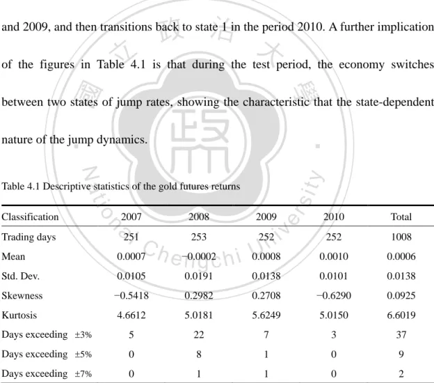
(33) Chapter 4 Empirical Analyses and Numerical Illustrations To investigate that the gold futures price follows the RSJM, we perform a strict empirical analysis for the gold futures returns. Applying the estimated parameters from the RSJM, this dissertation further provides some numerical illustrations using actual option market data to assess the impacts of both Merton measure and Esscher. 治政 transform on state-based jump-event premia. We also 大 present a comparative analysis 立 ‧. ‧ 國. 學. between alternative stochastic processes with respect to their pricing accuracy.. 4.1 Empirical results. sit. y. Nat. io. n. al. er. The dataset used in the descriptive analysis of Table 4.1 consists of the daily gold. i n U. v. futures prices. 2 Analyzing returns from different periods makes us to examine the. Ch. engchi. potential effect of different jump behaviors over time. The skewness and kurtosis coefficients suggest a leptokurtic distribution with positively skewed returns in the gold futures market. In 2008 and 2009, we can observe extreme movements and jumps in the daily returns, respectively. These can be regarded as the volatile state (state 2), whereas other periods can be viewed as the ordinary state (state 1). Taking. 2. The daily data are from Bloomberg and cover the period from 01/02/2007 to 12/31/2010. 24.

(34) the gold futures returns that are over ±5% in magnitude as an example, Table 4.1 shows that the mean frequency of the jumps in the entire period is 2.25, where the mean frequencies of the jumps in state 1 and state 2 are 0 and 4.5, respectively. State 1, therefore, is deduced as being below the long-term average jump activity. State 2 is inferred as being above the long-term average jump activity. As shown in Table 4.1, the period 2007 is in state 1, but the regime transitions to state 2 in the periods 2008. 政治大. and 2009, and then transitions back to state 1 in the period 2010. A further implication. 立. of the figures in Table 4.1 is that during the test period, the economy switches. ‧ 國. 學. between two states of jump rates, showing the characteristic that the state-dependent. ‧. nature of the jump dynamics.. y. Nat. Mean Std. Dev.. 2008. 2009. 253 252 i v n C U 0.0007 h e −0.0002 0.0008 ngchi. n. Trading days. 2007. a251 l. er. io. Classification. sit. Table 4.1 Descriptive statistics of the gold futures returns. 2010. Total. 252. 1008. 0.0010. 0.0006. 0.0105. 0.0191. 0.0138. 0.0101. 0.0138. Skewness. −0.5418. 0.2982. 0.2708. −0.6290. 0.0925. Kurtosis. 4.6612. 5.0181. 5.6249. 5.0150. 6.6019. Days exceeding ±3%. 5. 22. 7. 3. 37. Days exceeding ±5%. 0. 8. 1. 0. 9. Days exceeding ±7%. 0. 1. 1. 0. 2. Note: The descriptive statistics are reported for the gold futures returns from 2007 to 2010. This table shows the number of days each year in which the gold futures yield a logarithmic return series over ±3% , ±5% , and ±7% in magnitude.. 25.

(35) The previous analysis of Table 4.1 sheds doubts on the validity of the GBM assumption. Motivated by these findings, we examine the ability of alternative stochastic processes for modeling the gold futures prices. In the empirical analyses, we employ the Black–Scholes model (BSM) as a benchmark for the actual data analyzed. For simplicity, we assume that the hidden Markov chain X (t ) has two states: state 1 and state 2. This means that, an economy switches between the ordinary. 政治大. and volatile states. The transition probability matrix of the two-state Markov chain. 立P  = . ‧ 國. 12. P22 . P11 1 − P11  . Due to the economic state is hidden 1 − P P22   22. 學. P X (t ) is given by  11  P21. at time zero, the stationary distribution can be evaluated by the transition probability.. ‧. Therefore, the stationary distributions of state 1 and state 2 are π1 =. Nat. y. v2. v1 + v2. and. sit. n. al. er. io. π 2 = v1 v + v , respectively. Given the gold futures price dynamics defined in 1 2. i n U. v. Equation (2.5), we express the logarithmic return in discrete time as follows:. Ch.  N1 ( ∆t ) Y if ~ ~  k∑=1 k R(t ) =µ + σ Z +  N ( ∆t ) 2  ∑ Yk if  k =1. engchi X (t ) = 1. ,. (4.1). X (t ) = 2. ~ 1   where µ =  µ − σ 2 − Λκ  ∆t with Λ= κ 2  . ( p11λ1 + p22λ2 )(φY (1) − 1) ) , = σ σ ~. ∆t ,. Z ~ N (0,1) , Yk ~ N ( µ J , σ J2 ) , and N i (∆t ) is a Poisson process with the intensity rate. λi in the interval time ∆t when the Markov chain X (t ) remains in state i . The. 26.

(36) states and the jump arrivals are unobserved. We apply the EM algorithm (Lange, 1995a, b) to calculate the maximum likelihood estimations. In the first step, given the observed return data R and the former one-period parameters Θ( k −1) , we compute the conditional expectation of the log complete-data likelihood function as. = Γ ( Θ , Θ( k −1) ) E log Pr( R, X , N | Θ) | R, Θ( k −1)  . Then, for the second step, we maximize the Γ -function to use the parameter set as = Θ( k ) arg max Γ ( Θ , Θ( k −1) ) .. 政治大. By the iteration and recursive computation of these two steps, the parameters. 立. converge the Γ -function to the local maximum in the incomplete-data likelihood. ‧ 國. 學. function. Applying the code of the EM algorithm and the complete-data information. ‧. matrix, we get the standard errors of parameter estimators by the SEM algorithm. y. Nat. techniques. al. to. test. the. generalized. autoregressive. er. io. simulation. sit. (Meng and Rubin, 1991). Khalaf et al. (2003) combine bounds and Monte Carlo conditional. n. v i n Cclass heteroskedasticity (GARCH) with nuisance parameters. To determine h eofnmodels gchi U whether the JDM outperforms the BSM, and whether the data fit the RSJM better than the JDM, we apply the likelihood ratio test as follows:. asy. = LRΤ 2 ( ln L1 (Θ) − ln L0 (Θ) ) → χ d2,1−α ,. (4.2). where Lm (Θ) represents the likelihood function under the hypothesis H m for m = {0,1} , and d denotes the difference of the parameters between the H 0 and 27.

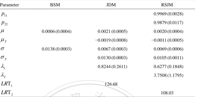
(37) H1 constraints. If LRΤ > χ d2,1−α , H 0 is rejected. The respective null hypotheses are that the BSM and JDM hold.. The estimated parameters and corresponding standard errors (in parentheses) for each one of the alternative stochastic processes, and the likelihood ratios under study are reported in Table 4.2. The results provide several interesting findings. In the case of the JDM vs. RSJM, we can determine the value of d by the difference in the number of. 治政 parameters between these two models. 大立. At the confidence level of. ‧ 國. 學. 2 1−α = 0.95 , the critical value for the aforementioned test is χ 4,0.95 = 9.49 . As shown. in Table 4.2, we can observe that the RSJM outperforms the JDM by the likelihood. ‧. ratio LRΤ2 of 108.03 > 9.49 at the 5% statistical significance level, implying that the. sit. y. Nat. io. n. al. er. addition of the Markov-modulated Poisson process clearly dominates the pure Poisson. i n U. v. process, that is, there exists the regime-switching jump feature due to the. Ch. engchi. state-dependent nature of the RSJM. By a similar procedure, we find that the JDM 2 clearly dominates the BSM by the likelihood ratio LRΤ1 of 126.68> χ 3,0.95 = 7.82. at the 5% statistical significance level, as shown in Table 4.2. In addition, these two transition probabilities of the gold futures market for the RSJM are almost 1, emphasizing that the economy stays in each state for a period of time and then transitions to other. Chang et al. (2013) indicate when the sum of these two transition. 28.

(38) probabilities is nearly 2, the autocorrelation of volatility (volatility clustering) is most significant. Table 4.2 shows that the sum of these two values is nearly 2, and we therefore find the volatility clustering is substantial, as in Chang et al. (2013). The mean and standard deviation of the gold futures returns for the RSJM are 0.0020 and 0.0069, respectively. The additional jump component prescribes a drift of −0.0011 and a volatility of 0.0105. The arrival intensity is found to be 0.6277 in state 1 and 3.7508. 政治大. in state 2, which clearly demonstrates different arrival rates in different states. These. 立. findings indicate that the gold futures price has a GBM structure with. ‧ 國. 學. Markov-modulated Poisson processes, that is, the jumps are subject to. ‧. regime-switching movements that cannot be explained by existing jump-diffusion. y. Nat. io. sit. processes, such as in Merton (1976), Amin (1993), and Kou (2002). They are. er. consistent with the findings in the descriptive analysis of Table 4.1, namely the. al. n. v i n C the non-normality of returns and U jump rates according to the h eexistence n g c hof ichanging economic states.. 29.

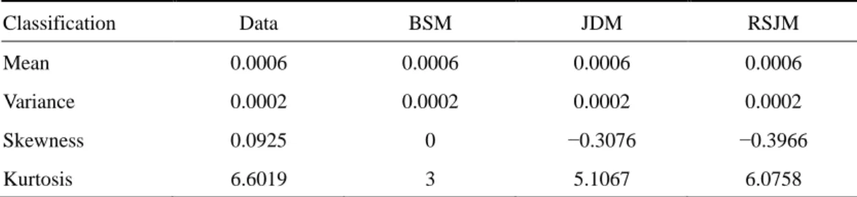
(39) Table 4.2 Estimated results of continuous-time models Parameter. BSM. JDM. RSJM. p11. 0.9969 (0.0028). p22. 0.9879 (0.0117). µ. 0.0006 (0.0004). µy σ σy. 0.0138 (0.0003). λ1 λ2. 0.0021 (0.0005). 0.0020 (0.0004). −0.0019 (0.0008). −0.0011 (0.0005). 0.0067 (0.0003). 0.0069 (0.0006). 0.0130 (0.0003). 0.0105 (0.0011). 0.8244 (0.2611). 0.6277 (0.1848) 3.7508 (1.1795). LRΤ1. 126.68. LRΤ2. 108.03 治政 Note: This table presents the empirical results of dynamic models, reporting the estimated parameters 大 and corresponding standard errors. The estimation settings for the BSM and JDM/RSJM are 立 determined via the maximum likelihood (ML) approach and EM algorithm, respectively. The standard. ‧ 國. 學. errors of parameter estimators for the BSM and JDM/RSJM obtained by the ML approach and SEM algorithm, respectively, are reported in parentheses. LRΤ1 represents the likelihood ratio test for. ‧. maximum likelihood functions with the null hypothesis that there is no jump event, that is, the dynamic model is BSM. LRΤ 2 shows the likelihood ratio test for maximum likelihood functions with the null. sit. y. Nat. hypothesis that there is no switching regime, that is, the dynamic model is JDM. Performance is. io. n. al. er. evaluated in terms of both the statistical accuracy and likelihood ratio test.. i n U. v. Table 4.3 presents the mean, variance, skewness, and kurtosis for the original. Ch. engchi. data and alternative stochastic processes. We further compare these model-determined values with empirical results. To investigate the leptokurtic and asymmetric features in gold futures returns, we use the formulas for the skewness and kurtosis of the JDM (Becker, 1981; Ball and Torous, 1983) and of the RSJM (Chang et al., 2013). As shown in Table 4.3, the mean and variance for the original data and alternative stochastic processes are the same. Comparing with the original data, the RSJM is. 30.

(40) better than BSM and JDM in terms of kurtosis.. Table 4.3 Distributional statistics for data and continuous-time models Classification. Data. BSM. JDM. RSJM. Mean. 0.0006. 0.0006. 0.0006. 0.0006. Variance. 0.0002. 0.0002. 0.0002. 0.0002. Skewness. 0.0925. 0. −0.3076. −0.3966. Kurtosis. 6.6019. 3. 5.1067. 6.0758. Note: This table reports the distributional statistics for the original data and continuous-time models.. 政治大. Figure 4.1 (a) plots the dynamic process of daily gold futures price data. Figure. 立. 4.1 (b) apparently exhibits different arrival rates with changing volatility over the test. ‧ 國. 學. period. The time-varying volatility is captured by the RSJM in the form of. ‧. regime-switching behavior, that is, the fluctuating periods of high and low arrival. Nat. io. sit. y. rates. Using the Baum-Welch algorithm adopted by Chang et al. (2013), as shown in. er. Figure 4.1 (c), we find that the first 150 and the last 450 days of the period seem to. al. n. v i n predominantly characterizedCbyha low arrival rate U e n g c h i (the probability of state 1 is close to. 1), while the other days are characterized by a high jump intensity (as in state 2). Our test period ends with a period of high arrival rates, corresponding to the U.S. subprime financial crisis of 2008. Figure 4.1 (d) shows the probability of jumps in a period, when there exists jumps, the probability is nearly 1. Compared with the Figure 4.1 (b), the aforementioned turmoil is an example of such jump-sensitive periods.. 31.

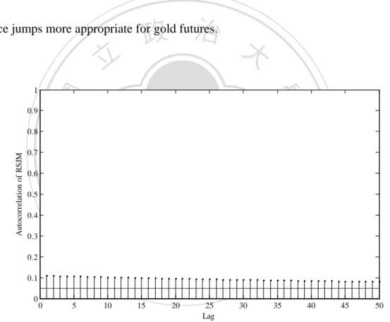
(41) Logarithmic Returns. 0.1. 1200 1000 800. 600 2007/01/022008/01/022009/01/022010/01/042010/12/31 Time (a) 1 0.8 0.6 0.4 0.2. 0 -0.05 -0.1 2007/01/032008/01/022009/01/022010/01/042010/12/31 Time (b) 1 0.8 0.6 0.4. 政治大. 0 2007/01/032008/01/022009/01/022010/01/042010/12/31 Time (c). 立. 0.05. The Probability of Jumps. 1400. The Probability of State 1. Gold Futures Prices (US$/Ounce). 1600. 0.3 2007/01/032008/01/022009/01/022010/01/042010/12/31 Time (d). Figure 4.1 Graph of (a) gold futures prices, (b) logarithmic returns, (c) State probability, and (d) Jump. ‧ 國. 學. probability. Note that the dotted lines in (b) denote the gold futures returns over ±5% in magnitude are jumps. (c). zero.. ‧. shows the probability of being in state 1, whereas the economy is in state 2 when the probability is. sit. y. Nat. io. n. al. er. Regarding the so-called volatility clustering, we make use of the autocorrelation. i n U. v. function of the squared asset returns calculated by Chang et al. (2013) to investigate. Ch. engchi. this phenomenon. Figure 4.2 shows a substantially positive autocorrelation in the squared logarithmic returns of gold futures in which the trend steadily declines as the lag length increases. The RSJM therefore captures not only the existence of volatility clustering but also the magnitude and decay of this phenomenon. Under the RSJM framework, the volatility clustering occurs from the jump clustering caused by the jump arrival intensity changes over time according to the states of an economy. These. 32.

(42) empirical results suggest that the RSJM provides the adequate description for the gold futures returns. It is an evidence that the model addresses the previously mentioned empirical characteristics, including the presence of jumps, leptokurtosis, asymmetry, and volatility clustering phenomena. The RSJM overcomes the shortcomings of GBM and jump-diffusion processes (Merton, 1976; Amin, 1993; Kou, 2002) for modeling the underlying asset price. This dynamic model will be general enough to cater for. 政治大. price jumps more appropriate for gold futures.. 立 0.8 0.7. sit. io. 0.4. n. al. er. 0.5. y. Nat. 0.6. ‧. ‧ 國. 0.9. Autocorrelation of RSJM. 學. 1. 0.3 0.2. Ch. 0.1 0. 0. 5. 10. 15. engchi 20. 25 Lag. i n U 30. Figure 4.2 Model autocorrelation of the squared logarithmic returns. 33. v. 35. 40. 45. 50.

(43) 4.2 Pricing performance. In this section, we evaluate the pricing performance of in-sample and out-of-sample periods using actual option market data 3 from the Commodity Exchange (COMEX). As a benchmark, we apply the BSM to price American put options on gold futures. The one-year U.S. treasury bill rate is used as a proxy for the risk-free rate. The relative mean square errors (RMSEs) are adopted for model evaluation. Due to actual. 治政 data limitations, an analysis across moneyness levels 大is not possible. The parameters 立 ‧ 國. 學. of each model are calibrated over periods of four years and then the estimated parameters are used to evaluate the pricing performance of in-sample and. ‧. out-of-sample periods for each option.. io. sit. y. Nat. er. The pricing errors presented in Table 4.4 correspond to RMSEs across both. al. n. v i n Cdata in-sample and out-of-sample U in-sample analysis of the option h eanalyzed. n g c hOni the pricing models in terms of RMSEs. The results show that the American gold put options are more accurately priced using the RSJM under the Esscher measure. For K = 780 and K = 800 , the pricing errors of the RSJM under the Esscher measure. are just slightly higher than those under the Merton measure in terms of RMSEs.. 3 The option data are from Bloomberg. These data correspond to the gold futures prices and cover the period between 10/01/2010 and 03/31/2011 with the expiration date 05/25/2011.. 34.

(44) Taking the strike price K = 860 as an example, the largest improvement offered by the RSJM under the Esscher measure over the Merton measure is 0.0411 in the reduction of RMSEs. Turning now to the out-of-sample analysis, we find a similar picture. The results show that the RSJM under the Esscher measure is again more accurate than under the Merton measure in pricing American gold put options. For K = 780 , the pricing error of the RSJM under the Esscher measure is just slightly. 政治大. higher than that under the Merton measure in terms of RMSEs. When K = 840 , the. 立. improvement is largest for the RSJM between the Esscher and Merton measures with. ‧ 國. 學. a reduction of 0.0672 in terms of RMSEs.. ‧. Through the analysis of in-sample and out-of-sample pricing errors with different. sit. y. Nat. io. n. al. er. strike prices K , these numerical illustrations indicate that pricing errors under the. i n U. v. RSJM are all smaller than those competing models in terms of RMSEs. Specifically,. Ch. engchi. the reduction of the RMSEs between the JDM and RSJM is more substantial than that of the RMSEs between the BSM and JDM. One can infer that for this reason, the Markov component contributes more to the superior pricing performance rather than the pure jump process. The numerical results show that the RSJM is more accurate than the BSM and JDM in pricing American gold put options. In other words, whether the Merton measure or Esscher transform is employed to derive the risk-neutral gold. 35.

(45) futures price dynamics, the RSJM strongly outperforms the BSM and JDM. Overall, the evidence presented seems to suggest that it is worth accounting for state-dependent jump risks when pricing American put options on gold futures. Once more data become available, it is necessary to engage a more extensive comparative analysis between alternative stochastic processes, not only with respect to their pricing accuracy but also in terms of their hedging performance.. 政治大. Table 4.4 In-sample and out-of-sample pricing errors of American gold put option pricing models BSM. 0.3549. 0.9587. 0.9542. 0.2910. 0.2935. 0.9429. 0.9376. 0.3176. 0.3008. 0.9231. 0.9174. 0.3512. 0.3202. 0.8985. 0.8930. 0.3836. 0.3425. y. sit. io. 860. 0.9659. 0.3583. er. 840. 0.9700. Nat. 820. Esscher measure. In-sample pricing errors (%) (Observations=64). ‧. 800. RSJM Merton measure. ‧ 國. 780. JDM. 學. K. 立. 820. 0.9909. 0.9882. 0.8288. 0.8100. 840. 0.9859. 0.9822. 0.9100. 0.8428. 860. 0.9796. 0.9737. 0.8454. 0.7900. n. 0.7089. 800. a lOut-of-sample pricing errors (%) (Observations=62) v i 0.9971 0.9955 0.7050 n Ch e 0.9925 n g c h i U 0.7622 0.9945. 780. 0.7423. Note: This table presents the RMSEs of various option pricing models. We calibrate each model in the period from 01/03/2007 to 12/31/2010 and then use the estimated parameters to evaluate the in-sample performance in the period from 10/01/2010 to 12/31/2010 as well as the out-of-sample performance in the period from 01/03/2011 to 03/31/2011. The RMSEs are estimated by minimizing the sum of the squared pricing errors between the LSM-simulated prices and the market prices (divided by the market prices) for each option. The RMSE (pricing error) expressed in percentage. Pricing performance is evaluated for the aggregate sample on the basis of the RMSEs.. 36.

(46) Chapter 5 Conclusions and Future Extensions According to the empirical analysis of the gold futures returns, we verify the existence of unanticipated jump events with different jump rates of gold futures prices in different time periods. The empirical results show that the gold futures price is better approximated by a continuous-time, Markov regime-switching jump-diffusion process.. 治政 Compared with the standard jump-diffusion processes, 大 the main advantage is that we 立 ‧ 國. 學. incorporate state-dependent jump risks into the dynamic model. This stochastic process also appropriately characterizes the leptokurtosis, asymmetry, and volatility. ‧. clustering across the empirical data analyzed. In the light of the empirically favored. sit. y. Nat. io. n. al. er. RSJM for the gold futures price under the different jump risk considerations, we adopt. i n U. v. the Merton measure and Esscher transform to derive the risk-neutral gold futures price. Ch. engchi. dynamics. After determining such dynamic processes, the values of American gold futures options are approximated using the LSM method. In this dissertation, we empirically investigate the in-sample and out-of-sample pricing performance of the LSM algorithm for American gold futures options with alternative stochastic processes, including GBM, JDM, and RSJM. The numerical results indicate that whether the Merton measure or Esscher transform is employed to derive the. 37.

(47) risk-neutral gold futures price dynamics, the RSJM strongly outperforms the BSM and JDM. As a consequence, we find that the Markov-modulated Poisson process is more accurate than the pure Poisson process when valuing American gold futures put options, and jump risks implied by the RSJM have a more significant impact on the option prices. To some extent, the comparison has indicated the importance of incorporating state-dependent jump risks into the gold futures price model.. 治政 This dissertation has several possible extensions 大 and potential improvements. 立 ‧ 國. 學. First, due to the discrete nature of jump risks, the riskless hedging with jump risks under an incomplete gold market remains an important challenge. Second, we might. ‧. employ an alternative distribution instead of a log-normal distribution used in the. sit. y. Nat. io. n. al. er. jump amplitude. Third, it is interesting to examine how the changing transition rate. i n U. v. impacts the transition probability under the measure change. Fourth, more simple, yet. Ch. engchi. powerful numerical algorithms are required to evaluate the American-style options. As a potential future work, we might consider incorporating other Markov regime-switching market parameters, such as interest rates, the appreciation rate and the volatility of the underlying asset price, the jump amplitude of a compound Poisson process, into the dynamic model studied in this dissertation. Comparing the effect of risk premia on the option prices may be a new interesting topic.. 38.

(48) References Amin, K. I., 1993. Jump diffusion option valuation in discrete time. The Journal of Finance 48, 1833–1863.. Ball, C. A., Torous, W. N., 1983. A simplified jump process for common stock returns. Journal of Financial and Quantitative Analysis 18, 53–65.. Ball, C. A., Torous, W. N., Tschoegl, A. E., 1985. An empirical investigation of the. 政治大. EOE gold options market. Journal of Banking and Finance 9, 101–113.. 立. Baur, D. G., Lucey, B. M., 2010. Is gold a hedge or a safe haven? An analysis of. ‧ 國. 學. stocks, bonds and gold. Financial Review 45, 217–229.. ‧. Baur, D. G., McDermott, T. K., 2010. Is gold a safe haven? International evidence.. y. Nat. n. er. io. al. sit. Journal of Banking and Finance 34, 1886–1898.. i n U. v. Beckers, S., 1981. A note on estimating the parameters of the diffusion jump model of. Ch. engchi. stock returns. Journal of Financial and Quantitative Analysis 16, 127–140.. Beckers, S., 1984. On the efficiency of the gold options market. Journal of Banking and Finance 8, 459–470.. Boyle, P., Broadie, M., Glasserman, P., 1997. Monte Carlo methods for security pricing. Journal of Economic Dynamics and Control 21, 1267–1321.. Brennan, M., Schwartz, E., 1977. The valuation of American put options. Journal of Finance 32, 449–462. 39.

(49) Capie, F., Mills, T. C., Wood, G., 2005. Gold as a hedge against the dollar. Journal of International Financial Markets, Institutions and Money 15, 343–352.. Carr, P., Geman, H., Madan, D., Yor, M., 2002. The fine structure of asset returns: an empirical investigation. Journal of Business 75, 305–332.. Chan, W. H., Maheu, J. M., 2002. Conditional jump dynamics in stock market returns. Journal of Business & Economic Statistics 20, 377–389.. 政治大 evidence for a Markov-modulated jump diffusion model of equity returns and 立. Chang, C., Fuh, C. D., Lin, S. K., 2013. A tale of two regimes: theory and empirical. derivative pricing implications. Journal of Banking and Finance 37, 3204–3217.. ‧ 國. 學. Cox, J. C., Ross, S. A., Rubinstein, M., 1979. Option pricing: a simplified approach.. ‧. Journal of Financial Economics 7, 229–263.. sit. y. Nat. n. al. er. io. Duan, J. C., Ritchken, P., Sun, Z., 2006. Approximating GARCH-jump models,. i n U. v. jump-diffusion processes, and option pricing. Mathematical Finance 16, 21–52.. Ch. engchi. Elliott, R. J., Chan, L., Siu, T. K., 2005. Option pricing and Esscher transform under regime switching. Annals of Finance 1, 423–432.. Elliott, R. J., Osakwe, C.-J. U., 2006. Option pricing for pure jump processes with Markov switching compensators. Finance and Stochastics 10, 250–275.. Elliott, R. J., Siu, T. K., Chan, L., Lau, J. W., 2007. Pricing options under a generalized Markov-modulated jump-diffusion model. Stochastic Analysis and Applications 25, 821–843. 40.

(50) Elliott, R. J., Siu, T. K., 2011. A risk-based approach for pricing American options under a generalized Markov regime-switching model. Quantitative Finance 11, 1633–1646.. Eraker, B., Johannes, M., Polson, N., 2003. The impact of jumps in volatility and returns. Journal of Finance 58, 1269–1300.. Eraker, B., 2004. Do stock market and volatility jump? Reconciling evidence from spot and option prices. Journal of Finance 59, 1367–1404.. 政治大 Gerber, H. U., Shiu, E. S. W., 1994. Option pricing by Esscher transforms (with 立 discussions). Transactions of Society of Actuaries 46, 99–191.. ‧ 國. 學. Gerber, H. U., Shiu, E. S. W., 1996. Actuarial bridges to dynamic hedging and option. ‧. pricing. Insurance: Mathematics and Economics 18, 183–218.. sit. y. Nat. n. al. er. io. Hull, J., White, A., 1990. Valuing derivative securities using the explicit finite. i n U. v. difference method. Journal of Financial and Quantitative Analysis 25, 87–100.. Ch. engchi. Khalaf, L., Saphores, J.-D., Bilodeau, J.-F., 2003. Simulation-based exact jump tests in models with conditional heteroskedasticity. Journal of Economic Dynamics and Control 28, 531–553.. Kou, S. G., 2002. A jump-diffusion model for option pricing. Management Science 48, 1086–1101.. Lange, K., 1995a. A gradient algorithm locally equivalent to the EM algorithm. Journal of the Royal Statistical Society 57, 425–437. 41.

(51) Lange, K., 1995b. A quasi-Newton acceleration of the EM algorithm. Statistica Sinica 5, 1–18.. Last, G., Brandt, A., 1995. Marked point processes on the real line: the dynamic approach. Springer-Verlag, New York.. Longstaff, F. A., Schwartz, E. S., 2001. Valuing American options by simulation: a simple least-squares approach. Review of Financial Studies 14, 113–147.. 政治大 components for individual stock returns. Journal of Finance 59, 755–793. 立. Maheu, J. M., McCurdy, T. H., 2004. News arrival, jump dynamics and volatility. ‧ 國. 學. McCown, J. R., Zimmerman, J. R., 2006. Is gold a zero-beta asset? Analysis of the investment potential of precious metals. Unpublished working paper, Oklahoma. ‧. City University. Available from http://ssrn.com/abstract=920496.. sit. y. Nat. n. al. er. io. McCown, J. R., Zimmerman, J. R., 2007. Analysis of the investment potential and. i n U. v. inflation-hedging ability of precious metals. Unpublished working paper,. Ch. engchi. Oklahoma City University. Available from http://ssrn.com/abstract=1002966.. Meng, X. L., Rubin, D. B., 1991. Using EM to obtain asymptotic variance-covariance matrices: the SEM algorithm. Journal of the American Statistical Association 86, 899–909.. Merton, R. C., 1976. Option pricing when underlying stock returns are discontinuous. Journal of Financial Economics 3, 125–144.. Ogden, J. P., Tucker, A. L., Vines, T. W., 1990. Arbitraging American gold spot and 42.

(52) futures options. Financial Review 25, 577–592.. Reboredo, J. C., 2013. Is gold a safe haven or a hedge for the US dollar? Implications for risk management. Journal of Banking and Finance 37, 2665–2676.. Zagaglia, P., Marzo, M., 2013. Gold and the U.S. dollar: tales from the turmoil. Quantitative Finance 13, 571–582.. 立. 政治大. ‧. ‧ 國. 學. n. er. io. sit. y. Nat. al. Ch. engchi. 43. i n U. v.

(53) Appendix A: Distributional properties of RSJM under. QM. Proof. Based on Equation (3.1), apply the Girsanov theorem and by the Itô's rule, we.    r  immediately get that W M (t )  W (t )   t is a Wiener process under Q M . We    then denote the moment-generating function of the random variable Yk by. Y (1)  E exp Yk     1 . This does not depend on the index k. because. 政治大. {Yk : k = 1, 2,...} all have the same distribution. Then, we have. 學. ‧ 國. 立.       (t )   n  E exp  Yk   P (t )  0  E exp  Yk  (t )  nP (t )  n  k 1   k 1     n1 . . I.  i Y (1).  exp t  ,. n. n0 i1 j 1. y. I. n. al. . Pij n, t . sit.  E exp Yk   P n, t  . io. n 0. n. er. . . ‧. . Nat. . . Ch. engchi. i n U. v. (A.1). where π i denotes the stationary distribution in state i . This limiting distribution can be computed by  jj i .  k1,k j kj  j. Furthermore, we note that. I. along with the constraint.  (t ).  k1 Yk t.  j1  j  1 . I. is a martingale at time t . Given. Φ (t ) = n , the Radon–Nikodym derivative of the transition probability can be written. as. 44.

(54) M dQ prob .. dPprob..  ( t )n.  1,. (A.2). then we get dP M (n, t )  dP(n, t ) , where P M (n, t ) denotes the transition probability matrix under Q M . Moreover, we use Equation (2.2) and its unique solution given by Equation (2.3). Letting P M (n, t )  P(n, t ) , we can get. . P. M*. ( , t ) . P. . M. (n, t ) . n0. n.  P(n, t ) n  P* ( , t ). 政治大 n0. 立. ‧ 國. 學.  exp    (1  ) t  ,. (A.3). ‧. Therefore, the transition rate matrix  of the transition probability matrix P M (n, t ). Nat. Finally, we investigate the jump amplitude, where. al. Y1 , Y2 ,, Yn  are independently. er. io. sit. y. and the arrival intensity matrix  M   are unchanged by the measure change.. n. v i n C hvariables. Thus, U identically distributed random e n g c h i the Radon–Nikodym derivative of each specific jump amplitude can be set as. dQYM dPY.  1,. (A.4). Ft X. then we obtain. dQYM. 2   Yk   y   M  dPY  exp   . Under Q , if a jump event 2 2  2 y  2 y  . 1. occurs at time k , the jump amplitude YkM is normally distributed with mean µ y 45.

(55) and variance σ y2 . Furthermore, under Q M , the density function of each specific jump amplitude YkM is fYM ( y )  fY ( y ) , and therefore the density function is unchanged by the change of measures.. 立. 政治大. ‧. ‧ 國. 學. n. er. io. sit. y. Nat. al. Ch. engchi. 46. i n U. v.

(56) Appendix B: Solving the Esscher parameters Proof. Let Eθ. m. denote the mathematical expectation operator with respect to the. Esscher measure Qθ. m. equivalent to P . It is possible to select the risk-neutral. Esscher measure as the measure Qθ. m. such that the discounted gold futures price. process is a Qθ -martingale. This is obtained by determining the Esscher parameters m. θ C and θ J as solutions of E  exp rt  F (t ) F0   F (0) . Applying Equation (3.4), m. we have. 政治大. F (0)  exp rt  E. m. 學. ‧ 國. 立.  dQ m      F (t ) F0   exp rt  E  F t F ( ) 0  dP      . ‧ y. Nat.  (t )    dQ m   1  2    F (0) E  exp   r    t  W (t )  Yk         2 dP     k 1. n. al. er. io. sit. . v i n Ch e n g c h i U . 2  2   1 1 1  F (0) exp   r   2  t  1   C   t   C   t    2 2 2 . J     1 J   exp       t  ,   . (B.1). From the mutual independence of random shocks W (t ) , Φ (t ) , and Yk , and then the martingale condition holds if and only if the Esscher parameters θ C and θ J satisfy.   r    C  2  0. (B.2). 47.

(57) and. 1  y   2y   J  2y  0 , 2. (B.3). for all t ∈ [ 0, T ] . Therefore, we can define a pair of solutions of Esscher parameters for the martingale condition by Equations (3.5) and (3.6).. 立. 政治大. ‧. ‧ 國. 學. n. er. io. sit. y. Nat. al. Ch. engchi. 48. i n U. v.

(58) Appendix C: Distributional properties of RSJM Qθ. under. m. Proof. By Equation (3.4), apply the Girsanov theorem and from the mutual independence of random shocks W (t ) , Φ (t ) , and Yk , we can obtain that W θ= (t ) W (t ) − θ Cσ t is a Wiener process under Qθ . Next, we denote the m. m. moment-generating. function. of. the. random. variable. 政治大. by. Yk. J Y ( J )  E  exp  J Yk      1 . This does not depend on the index k because  . 立. {Yk : k = 1, 2,...}.      (t )   E exp  J Yk   P (t )  0  E exp  J  k 1     n1 . . . n0. . I. sit. a l. . I. er. n. E  exp  J Yk  P(n, t )   . n. . io. . . y. Nat. .   Yk  (t )  nP (t )  n   k 1 n. ‧. ‧ 國. 學. all have the same distribution. Then, we have.  i Y (i vJ ) C h n0 i1 j1 U n engchi. n. Pij (n, t ). .  exp   t , J. (C.1). where π i denotes the stationary distribution in state i . This limiting distribution can be computed by  jj i .  k1,k j kj  j I. Specifically, we note that  J. along with the constraint.  (t ).  k1 Yk  t J.  j1  j  1 . I. is a martingale at time t . Given. Φ (t ) = n , the Radon–Nikodym derivative of the transition probability can be set as. 49.

(59) dQprob. m. dPprob.. . n.  ( t )n. .  Y ( J ) exp   t , J. (C.2). . . then we get dP (n, t )  dP(n, t ) Y ( J ) exp   t , where Pθ (n, t ) denotes n. m. J. m. the transition probability matrix under Qθ . We use Equation (2.2) and its unique m. . . solution given by Equation (2.3). Letting P (n, t )  P(n, t ) Y ( J ) exp   t , n. m. J. we can get. P.  * m. 政治大 ( , t )   P(n, t )  ( ) exp  t     P(n, t )  ( ) exp  t  立 . n. J. J. . n. J. Y. n0. J. n0. . 學. ‧ 國. n. Y. .  exp    (1  )Y ( J ) t ,. (C.3). ‧. where the transition rate matrix  of the transition probability matrix P (n, t ) is. Nat. sit. y. m. unaffected by the Esscher transform. Under Qθ , the jump risk can be formulated by. io. er. m. 2 m  1 the Esscher transform intensity   Y ( J )   exp  J  y   J  y   . Finally,   2. n. al. Ch. engchi. we investigate the jump amplitude, where. i n U. v. Y1 , Y2 ,, Yn  are independently. identically distributed random variables. Hence, the Radon–Nikodym derivative of each specific jump amplitude can be written as. dQY dPY. m.  Ft X. exp  J Yk    E  exp  J Yk  X   F0  . ,. (C.4). 50.