依據製程能力指標 Cpmk 應用複式抽樣方法於供應商選擇

(1)

國立交通大學

工業工程與管理學系

碩士論文

依據製程能力指標

C

_pmk

應用複式抽樣方法於

供應商選擇

Bootstrap Approach for Supplier Selection Based on

Process Capability Index

C

_pmk

研究生：邱勝亮

指導教授：彭文理博士

吳建瑋博士

(2)

依據製程能力指標

C

_pmk

應用複式抽樣方法於

供應商選擇

Bootstrap Approach for Supplier Selection Based on

Process Capability Index

C

_pmk

研究生：邱勝亮 Student : Sheng-Liang Chiu 指導教授：彭文理博士 Advisor : Dr. W. L. Pearn 吳建瑋博士 Dr. Chien-Wei Wu

國立交通大學

工業工程與管理學系

碩士論文

A Thesis

Submitted to Department of Industrial Engineering and Management

College of Management

National Chiao Tung University

in partial Fulfillment of the Requirements

for the Degree of

Master

in

Industrial Engineering

May 2007

Hsinchu, Taiwan, Republic of China

(3)

依據製程能力指標

C

_pmk

應用複式抽樣方法於

供應商選擇

研究生：邱勝亮指導教授：彭文理博士

吳建瑋博士

國立交通大學工業工程與管理學系碩士班

摘要

製程能力指標是藉由一個指標值來衡量製程的能力與產品的品質，過去學者對於以製程能力指標來衡量兩家供應商製程的問題已經提出了一些方法。然而，依據製程能力指標 C_pmk 於供應商選取的問題目前尚未被研究。這個指標的建構結合了 C_pk 與 C_pm 兩個指標的優點，同時考量到製程良率以及製程損失的特性。本篇論文的研究目的就是在兩家相互競爭的供應商之間選出一家具有較好製程能力的供應商，並建立了一個依據 C_pmk 指標的決策程序供使用者於決策時使用。本研究是應用複式抽樣的方法針對兩供應商之製程間的檢定統計量來估計信賴下界，藉由比較四種複式抽樣信賴區間的錯誤機率和篩選檢定力後，結果發現以偏誤校正的比例複式抽樣法 (BCPB) 在相同的樣本數下有較穩定的錯誤機率以及比較顯著的篩選檢定力。所以在這四種複式抽樣方法中，BCPB 之複式抽樣法為表現比較好的方法。最後，為了實務應用上的便利，我們提供一個供應商選取程序作為選取決策之參考。關鍵字：製程能力分析、供應商選擇、複式抽樣法、錯誤機率、篩選檢定力。 i

(4)

Bootstrap Approach for Supplier Selection Based

on Process Capability Index

C

_pmk

Student: Sheng-Liang Chiu

Advisor：

.

Dr. W. L. Pearn

Dr. Chien-Wei Wu

Department of Industrial Engineering and Management

National Chiao Tung University

Abstract

Process capability indices (PCIs) intended to provide single-number assessments of ability to meet specification limits on quality characteristics. Many individuals have indicated various approaches for supplier selection or process comparison problem based on PCIs. However, the method of supplier selection based on process capability index C_pmk is not yet investigated. The index is constructed by combining the yield-based index C_pk and the loss-based index C_pm, taking into account the process yield as well as the process loss. The principal purpose of this thesis is to determine the more capable process between two competing suppliers and provide the supplier selection procedure based on C_pmk

index for practical applications. In this study, we apply the bootstrap method, a data-based simulation technique, to construct lower confidence bound for the statistics between two suppliers. A comparison among four bootstrap methods is also analyzed by evaluating the error probability and the selection power. The result indicates that the BCPB method is the better approach among four bootstrap methods for process comparison due to its stable error probability and larger selection power with a fixed sample size. Finally, for convenience of applications, a practical step-by-step testing procedure for engineers is implemented to refer to supplier selection decisions.

Key words: bootstrap method, error probability, process capability indices, selection power, supplier selection.

(5)

誌謝

這篇碩士論文的完成，首先要感謝我的指導教授彭老師，老師在做

研究上一向要求嚴謹，也因為這樣的態度，才能有顯著的學術成就。

在對待學生上，除了對我們論文的要求外，寶貴的人生經驗談與做事、

做學問的態度，是我兩年內最大的收穫。

此外，建瑋學長，感謝給了我許多論文上的建議，還不辭辛苦的

往返台中，新竹兩地，鍾老師在口試上也幫了我很多的忙。博班的學

長、學姊們，MB517、519、516 的研究室夥伴們，很高興和大家一起相

處，使我這兩年過得多采多姿。

最後，謝謝我的爸爸、媽媽，讓我可以在舒適、安逸的環境學習，

希望他們保持身體健康，天天快樂。

iii

(6)

Abstract (Chinese)

... i

Abstract

... ii

誌謝

... iii

List of Table

... v

List of Figure

... vi

Notations

... x

1. Introduction

... 1 1.1 Motivation ... 1 1.2 Research Objectives ... 1 1.3 Research Structure ... 2

2. Literature Review

... 4

2.1 Process Capability Indices... 4

2.2 The Method of Selecting the Better Supplier Based on PCIs ... 5

2.3 Process Yield Based on C_pmk Index... 6

3. Selection Method

... 8

3.1 Difference Test on Comparing Two C_pmk Indices... 8

3.2 Ratio Test on Comparing Two C_pmk Indices ...10

3.3 Bootstrap Methodology...10

4. Performance Comparison of Four Bootstrap Methods

...14

4.1 Simulation Layout Setting...14

4.2 Error Probability Analysis...16

4.3 Selection Power Analysis ...19

5. Supplier Selection Based on BCPB Method

...22

5.1 Sample Size Determination with Designated Selection Power...22

5.2 Selection Procedure of Two Competing Suppliers...24

6. Application

Example

...26

6.1 Application Example of FPC ...26

6.2 Data Analysis and Supplier Selection ...28

7. Conclusions

...31

References

...32

Appendix A. Error probability analysis information

...34

Appendix B. Power analysis information

...38

(7)

List of Table

Table 1. Bounds on %NC and C_a for C_pk =C_pmk =C ... 7

Table 2. C values and ranges of μ ...14 _a Table 3. Parameter values for two manufacturing suppliers used in the simulation study under C_pmk₁ =C_pmk₂ =1.00...15

Table 4. The results of error probability analysis for difference test ...18

Table 5. The results of error probability analysis for ratio test...18

Table 6. Simulation results of the four bootstraps methods for the difference and ratio statistics ...19

Table 7. Sample size required of BCPB method for the difference statistics under 0.05 α= , with power = 0.90, 0.95, 0.975, 0.99, C_pmk₁ =1.00, ...22 2 1.05(0.05)1.50 pmk C = Table 8. Sample size required of BCPB method for the ratio statistics under 0.05 α= ,with power = 0.90, 0.95, 0.975, 0.99, C_pmk₁=1.00, ...23 2 1.05(0.05)1.50 pmk C = Table 9. Sample size required of BCPB method for the difference statistics under 0.05 α= , with power = 0.90, 0.95, 0.975, 0.99, C_pmk₁ =1.33, ...23 2 1.43(0.05)1.83 pmk C = Table 10. Sample size required of BCPB method for the ratio statistics under 0.05 α= ,with power = 0.90, 0.95, 0.975, 0.99, C_pmk₁=1.33, ...23 2 1.43(0.05)1.83 pmk C = Table 11. Sample data of supplier I ...28

Table 12. Sample data of supplier II ...29

Table 13. The outcome of Shapiro-Wilk test ...30

Table 14. The sample statistics for two suppliers ...30

Table 15. The error probability of four bootstrap methods for the difference and ratio test with 16 combinations of (Ca1,σ2) and (Ca2,σ2) under 1 pmk C =C_pmk₂=1 ...34

Table 16. Selection power of the four bootstrap methods for the difference and ratio statistic for on-target process with μ1 =μ2 = and sample size 0 =10(10)200...38

n Table 17. Selection power of the four bootstrap methods for the difference and ratio statistic for off-target process with μ1 =μ2 =0.4 and sample size =10(10)200...44

n

(8)

List of Figure

Figure 1. Illustration of research structure ... 3

Figure 2. Four processes with C_pmk =1.00...15

Figure 3. Error probability of four bootstraps under C_pmk₁=C_pmk₂ =1.00...17

Figure 4. Error probability of four bootstraps under C_pmk₁/C_pmk₂ =1.00...17

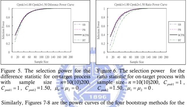
Figure 5. The selection power for the difference statistic for on-target process with sample size n=10(10)200, C_pmk₁ =1, C_pmk₂=1.50, μ₁ =μ₂ =0 ...20

Figure 6. The selection power for the ratio statistic for on-target process with sample size =10(10)200, n C_pmk₁=1, C_pmk₂=1.50, μ₁=μ₂ =0 ...20

Figure 7. The selection power for the difference statistic for off-target process with sample size n=10(10)200, C_pmk₁ =1, C_pmk₂=1.50, μ₁ =μ₂ =0.4 ...20

Figure 8. The selection power for the ratio statistic for off-target process with sample size = 10(10)200, n C_pmk₁=1, C_pmk₂=1.50, μ₁ =μ₂ =0.4 ...20

Figure 9. The sample size curve for the difference statistic under α=0.05, with power = 0.90, 0.95, 0.975, 0.99, C_pmk₁ =1.00, C_pmk₂ =1.15(0.05)1.50 ...24

Figure 10. The sample size curve for the ratio statistic under α=0.05,with power = 0.90, 0.95, 0.975, 0.99, C_pmk₁ =1.00, C_pmk₂ =1.15(0.05)1.50 ...24

Figure 11. The sample size curve for the difference statistic under α=0.05, with power = 0.90, 0.95, 0.975, 0.99, C_pmk₁ =1.33, C_pmk₂ =1.48(0.05)1.83..24

Figure 12. The sample size curve for the ratio statistic under α=0.05, with power = 0.90, 0.95, 0.975, 0.99, C_pmk₁ =1.33, C_pmk₂ =1.48(0.05)1.83 ...24

Figure 13. Coverlay Type - Single Sided FPC ...27

Figure 14. 0.5 mm SMT FPC Connector —— Straight ...27

Figure 15. The layout of the SMT type of 0.5 mm FPC Connector and 0.3 mm thickness FPC ...27

Figure 16. Histogram of supplier I data ...29

Figure 17. Histogram of supplier II data ...29

Figure 18. Normal probability plot for supplier I ...30

Figure 19. Normal probability plot for supplier II ...30

Figure 20. The difference statistic with sample size =10(10)200, , , n C_pmk₁=1 2 1.05 pmk C = μ₁=μ₂ =0 ...50

Figure 21. The ratio statistic with sample size =10(10)200, , , n C_pmk₁ =1 2 1.05 pmk C = μ₁=μ₂ =0 ...50 vi

(9)

Figure 22. The difference statistic with sample size n=10(10)200, C_pmk₁=1, 2

pmk

C =1.10, μ₁=μ₂ =0 ...50 Figure 23. The ratio statistic with sample size =10(10)200, n C_pmk₁ =1,

2

pmk

C =1.10, μ₁=μ₂ =0 ...50 Figure 24. The difference statistic with sample size n=10(10)200, C_pmk₁=1,

2

pmk

2

pmk

C =1.15 , μ₁ =μ₂ =0 ...51 Figure 26. The difference statistic with sample size n=10(10)200, C_pmk₁=1,

2

pmk

2

pmk

2

pmk

2

pmk

2

pmk

C =1.30, μ₁=μ₂ =0 ...52 Figure 31 . The ratio statistic with sample size =10(10)200, n C_pmk₁=1,

2

pmk

2

pmk

2

pmk

2

pmk

2

pmk

2

pmk

2

pmk

2

pmk

2

pmk

C =1.50, μ1=μ2 = ...53 0

(10)

Figure 40. The difference statistic with sample size =10(10)200, , , n C_pmk₁=1 2 1.05 pmk C = μ1=μ2 =0.4...54 Figure 41. The ratio statistic with sample size =10(10)200, ,

,

n C_pmk₁ =1

2 1.05

pmk

C = μ1=μ2 =0.4...54 Figure 42. The difference statistic with sample size n=10(10)200, C_pmk₁=1,

2

pmk

C =1.10, μ1=μ2 =0.4 ...54 Figure 43. The ratio statistic with sample size =10(10)200, n C_pmk₁ =1,

2

pmk

C =1.10, μ1=μ2 =0.4 ...54 Figure 44. The difference statistic with sample size n=10(10)200, C_pmk₁=1,

2

pmk

2

pmk

C =1.15, μ1=μ2 =0.4 ...55 Figure 46.The difference statistic with sample size n=10(10)200, C_pmk₁ =1,

2

pmk

2

pmk

2

pmk

2

pmk

2

pmk

2

pmk

2

pmk

2

pmk

2

pmk

2

pmk

2

pmk

2

pmk

C =1.45, μ1=μ2 =0.4 ...57

(11)

Figure 58. The difference statistic with sample size n=10(10)200, C_pmk₁=1, 2

pmk

2

pmk

C =1.50, μ1=μ2 =0.4 ...57

(12)

Notations

T : target

LSL : the lower specification limits preset by the process engineers USL : the upper specification limits preset by the process engineers

d : the half specification width

m : the midpoint between the upper and the lower specifications limits μ _{: the population mean}

2

σ : the population variation

σ : the population standard deviation %NC : the fraction of Non-Conformities

n : the number of the sample size drawn from suppliers

B : the number of bootstrap resamples

N : simulation replicated times

1 ˆ

pmk

C : the Cˆpmk1 of bootstrap resamples from supplier I

2 ˆ

pmk

C : the Cˆ_pmk₂ of bootstrap resamples from supplier II

θ : the difference or the ratio of two suppliers’ C_pmk index ˆ

θ : the estimator of θ *

ˆ

θ : the associated ordered bootstrap estimate of θ *

ˆ

θ : the sample average of the B bootstrap estimates *

(13)

1. Introduction

1.1 Motivation

Over past decades, there are remarkable developments in the field of process capability indices (PCIs). PCIs are intended to provide single-number assessments of ability to meet specification limits on quality characteristics (Kotz and Johnson (2002)). On the other hand, the trend of vertical integration between suppliers and manufacturers has been developed. Supplier selection problem plays a critical role in modern manufacturing environment. It has been proposed that process capability index is the most precise and effective assessment for the determination of the better supplier.

Many individuals have indicated various approaches for supplier selection or process comparison problem based on PCIs. For the index C_p, Tseng and Wu (1991) and Chou (1994) used modified likelihood ratio and likelihood ratio test respectively to compare processes. For the index C_pk, Chen ant Tong (2003) constructed the biased corrected percentile bootstrap (BCPB) confidence interval of (C_pk₁−C_pk₂) to select the better of two suppliers and Daniels et al. (2005) accessed the Bonferroni method to select suppliers. For the index C_pm, Huang and Lee (1995), Pearn et al. (2004) and Chen and Chen (2004a) suggested looking for the smallest _γ2 ₌_{E X T}₍ ₋ ₎2 ₌_σ2₊₍_μ₋_T₎2_{, two-phase selection procedure} and ratio test method respectively for supplier selection. Although a lot of investigation on supplier selection based on PCIs has been done so far, discussion relative to the subject based on the index C_pmk has not been concentrated on. With the merit of combining process yield and process loss, more studies need to be conducted for the method of supplier selection based on C_pmk index.

1.2 Research Objectives

The purpose of this thesis is to determine the more capable process between two competing suppliers based on C_pmk index. Owing to the complexity of sampling distribution, we apply the bootstrap method, a data-based simulation technique, to construct lower confidence bound for the statistics between two suppliers. A comparison among four bootstrap methods is also analyzed by evaluating the error probability and the selection power. After the analysis of the

(14)

simulation outcome, this study provides sample size tables for conducting hypothesis test and the supplier selection procedure based on C_pmk index for current manufacturing industries.

1.3 Research Structure

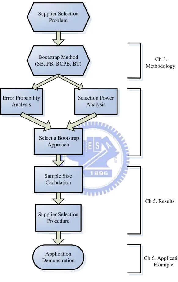
In this section, it has been shown a brief review of our research about bootstrap approach for supplier selection based on process capability index C_pmk. A summary of the substance for each chapter is presented below; and further, the research structure is illustrated in Figure 1.

Ch1. Introduction: Serve as an orientation for readers to understand summary knowledge about PCIs and bootstrap.

Ch2. Literature review: A review of the characteristics and formulations of PCIs in the first part. For the second part, review papers about supplier selection based on PCIs has been summarized.

Ch3. Selection Method: Introduce the approach of formulating hypothesis tests and bootstrap sampling methodology.

Ch4. Performance Comparison of Four Bootstrap Methods: Apply simulation technique to compare four bootstrap methods based on error probability and selection power analysis.

Ch5. Supplier Selection Based on BCPB Method: According to the results of performance comparison in Chapter 4, sample size tables and selection procedure are provided.

Ch6. Application Example: Take an example from FPC industry to illustrate supplier selection method in this thesis.

Ch7. Conclusion: Take a broad look at our findings for the specific supplier selection problem.

(15)

Supplier Selection Problem Bootstrap Method (SB, PB, BCPB, BT) Error Probability Analysis Selection Power Analysis Select a Bootstrap Approach Sample Size Caclulation Supplier Selection Procedure Application Demonstration Ch 3. Methodology Ch 5. Results Ch 6. Application Example

Figure 1. Illustration of research structure.

(16)

2. Literature Review

2.1 Process Capability Indices

Process Capability Indices are intended to provide single-number assessments of ability to meet specification limits on quality characteristics (Kotz and Johnson (2002)). It has been proposed in the manufacturing industry to measure on whether a process is capable of reproducing items or not. A review in this section is going to describe some and current development in PCIs. The use of process capability indices began in United States during early 1980s. Many authors have promoted the use of various PCIs for evaluating a supplier’s process capability. Examples include Boyles (1991), Pearn et al. (1992), Kushler and Hurley (1992), Kotz and Johnson (1993), Vännman and Kotz (1995), Vännman (1997), Kotz and Lovelace (1998), Pearn et al. (1998), Kotz and Johnson (2002), Pearn and Shu (2003) and references therein. A general acceptance of the idea that PCIs can be used only after it have been established that a process is in statistical control and an assumption that the measured characteristics should have a normal distribution (at least, approximately). Four well-known capability indices have been defined respectively as (Juran (1974), Pearn et al. (1998), Kane (1986), and Hsiang and Taguchi (1985)):

6 p USL LSL C σ − = , | | 1 a m C d μ− = − , =min , | | 3 3 3 pk USL LSL d m C μ μ μ σ σ σ ⎧ − − ⎫₌ − − ⎨ ⎬ ⎩ ⎭ , 2 2 6 ( pm USL LSL C T σ μ ) − = + − ,

where μ is the process mean, is the upper specification limit, is the lower specification limit,

USL LSL

σ is the process standard deviation, T is target value,

(

)

2

d = USL LSL− , and m=

(

USL LSL+

)

2. The C_p index reflects product consistency by evaluating the overall process variability relative to the manufacturing tolerance. The index measures the degree of process centering, which can be regarded as a process accuracy index. The

a

C

pk

C index evaluates process variation and the location of the process mean to offset some of the weakness in C_p and , which is a yield-based index (see Boyles (1991)) providing lower bounds on process yield. The

a

C

pm

C index incorporate with the variation of production items with respect to the target value and specification limits preset in the factory. Since the design is based on the average process loss,

(17)

which has been called the Taguchi index.

Many process capability indices, such as C_p, C_a, C_pk and C_pm, have been proposed to provide numerical measures. Combining the advantages of these indices, Pearn et al. (1992) introduced a new capability index called C_pmk. It is

2 2 2 2 min , 3 ( ) 3 ( ) pmk C T T σ μ σ μ = _⎨ _⎬ + − + − ⎪ ⎪ ⎩ ⎭ USL μ μ LSL ⎧ ₋ ₋ ⎫ ⎪ ⎪_.

It is constructed by combining the yield-based index C_pk and the loss-based index C_pm, taking into account the process yield as well as the process loss. When the process mean μ depart from the target value T, the reduced value of

pmk

C is more significant than those of Cp, Cpk and Cpm. And it remains

sensitive to the shift of process variation. Clearly C_p ≥C_pk ≥C_pmk and

p pm pmk

C ≥C ≥C . The relation between C_pk and C_pm is less clearcut. If the process meets the capability requirement ‘ ’, then the process must meet both capability requirements ‘ ’ and ‘ ’ since

pmk C ≥ C C C pk C ≥ C_pm ≥ C_pm ≥C_pm_k and pk pm

C ≥C _k (Pearn and Lin (2002)). While C_pk remains the more widely used index, Cpmk is considered to be an advanced and useful index for processes with

two-sided specification limits.

2.2 The Method of Selecting the Better Supplier Based on PCIs

With the improvement of technology, it is more important to enhance quality and satisfy the customer’s requirements. Judging the better of suppliers is the critical issue. A review of the literature indicates that many approaches have been applied for supplier selection. Tseng and Wu (1991) considered the problem for available manufacturing processes based on the precision index k C_p under a modified likelihood ratio (MLR) selection rule. Chou (1994) used the likelihood ratio test (LRT) to compare two processes for the unilateral cases that two sample sizes are equal and developed F test to compare two suppliers based on C_p. Huang and Lee (1995) selected the supplier by searching the largest C_pm which are used to looking for the smallest _γ2 ₌_{E X T}₍ ₋ ₎2 ₌_σ2 ₊₍_μ₋_T₎2

2

. The purpose was to select a subset containing the processes from given independent process. Chen and Tong (2003) proposed a bootstrap re-sampling simulation method to construct the biased corrected percentile bootstrap (BCPB) confidence interval of (C_pk₁−C_p_k ) to select the better of two suppliers. Furthermore, Pearn et al. (2004) implemented this method which developed a two-phase selection procedure to select a better supplier and examine the magnitude of the difference between the two suppliers. Chen and Chen (2004a) judged the better of two processes based

(18)

on a confidence interval for the ratio C_pm₁/C_pm₂. Four methods are presented and compared. One based on the statistical theory given in Boyles (1991) and three based on the bootstrap, (referred to as SB, PB and BCPB). Chen and Chen (2004b) developed approximately F test to determine whether or not two processes are equally capable based on C_pm. Daniels et al. (2005) considered the Bonferroni, Modified Bonferroni, Difference, Ratio and General Confidence Interval methods to construct confidence intervals for performing these comparisons on C_pk and

pm

C . Chen and Chen (2006) applied the process incapability index C_pp to develop an evaluation model that assesses the quality performance of suppliers. However, difference and ratio test for supplier selection based on C_pmk have not been developed due to the complexity of its sampling distribution. This study applies the bootstrap re-sampling simulation to compare two processes based on

pmk

C .

2.3 Process Yield Based on Cpmk Index

For most supplier selection problem in manufacturing factories, increasing the product yield or reducing the percentages of non-conforming items is the primary concern for quality improvement. Motorola’s “Six Sigma” program essentially requires the process capability at least 2.0 to accommodate the possible 1.5σ process shift (see Harry (1988)), and no more than 3.4 ppm are defectives. The most natural measure is the proportion itself called the yield, which we refer to Yield defined as:

( ) ( ) ( )

USL LSL

Yield =

_∫

dF x =F USL −F LSL ,

where F x( ) is the cumulative distribution function of the measured characteristic X . If the process characteristic X follows _N_{( ,}_{μ σ}2₎_{, then the} fraction of nonconformities NC is:

%NC 1 USL μ μ LSL σ σ − − ⎛ ⎞ ⎛ ⎞ = − Φ_⎜ _⎟+ Φ_⎜ _⎟ ⎝ ⎠ ⎝ ⎠.

The index C_pk provides bounds on process yield for a normally distributed process. Given fixed value of C_pk, the bounds are 2 (3Φ C_pk) 1− ≤ yield ≤ Φ(3C_p_k)

(Boyles(1991)) or Φ −( 3C_pk) %≤ NC ≤ Φ −2 ( 3C_pk) for ≤0 C_a ≤ , where 1 is the cumulative distribution function (CDF) of the standard normal distribution

. For

( ) Φ ⋅ ( 0,1)

N C =_pk 1.00, one would expect that the fractions of defectives is no more than 2700 ppm. It is presently not clear whether or not the index C_pmk is related to the process yield, since the relationship between C_pmk and process

(19)

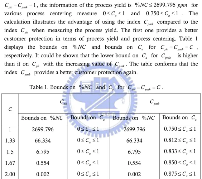
yield has not been developed. Pearn and Lin (2005) have provided a mathematically derivation of an upper bound formula on process yield in terms of the percentage of nonconformities. The bounds are:

0 %≤ NC ≤ Φ −2 ( 3C_pmk) for C_pmk ≥ 2 /3.

These results conform that the two indices, C_pk and C_pmk provide the same upper bounds on the percentage of nonconformities. For instance, given

, the information of the process yield is

1

pk pmk

C =C = %NC ≤2699.796 ppm for

various process centering measure 0≤C_a ≤ and 1 . The calculation illustrates the advantage of using the index

0.750≤C_a ≤1

pmk

C compared to the index C_pk when measuring the process yield. The first one provides a better customer protection in terms of process yield and process centering. Table 1 displays the bounds on %NC and bounds on for , respectively. It could be shown that the lower bound on for

a

C C_pk =C_pmk =C

a

C C_pmk is higher than it on C_pk with the increasing value of C_pmk. The table conforms that the index C_pmk provides a better customer protection again.

Table 1. Bounds on %NC and C_a for C_pk =C_pmk =C .

pk

C C_pmk

C

Bounds on %NC Bounds on C Bounds on %NC Bounds on a C a

1 2699.796 0≤C_a ≤ 1 2699.796 0.750≤C_a ≤ 1 1.33 66.334 0≤C_a ≤ 1 66.334 0.812≤C_a ≤ 1 1.5 6.795 0≤C_a ≤ 1 6.795 0.833≤C_a ≤ 1 1.67 0.554 0≤C_a ≤ 1 0.554 0.850≤C_a ≤ 1 2.00 0.002 0≤C_a ≤ 1 0.002 0.875≤C_a ≤ 1 7

(20)

3. Selection Method

3.1 Difference Test on Comparing Two Cpmk Indices

The process capability indices can be used to determine the more capable of competing processes. Since we have no direct observation of the entire processes, we do not know which process is more capable (Chou (1994)). In practice, real process measurements μ and _{σ are unknown. We could gather sample data}2 to determine index values. The indices calculated from the sample data cannot be immediately used to determine which supplier is better because sampling errors may lead to an uncorrected result. The difference hypothesis testing approach is used here to enhance reliability.

We investigate the selection problem for cases with two candidate processes based on the C_pmk index. Let π_i be the population assumed to be normally distributed with mean μ_i and variance 2

i

σ , i =1, 2, and are the independent random samples from

1, 2,..., i

i i in

x x x

i

π , i =1, 2. In most applications, if a new supplier II wants to compete for the orders by claiming that its capability is better than the existing supplier I, then the new S2 must furnish convincing information justifying the claim with a prescribed level of confidence. Thus, the supplier selection decisions would be based on the hypothesis testing comparing the two

pmk C values. It is 0: pmk1 pmk2 H C ≥C 1: pmk1 pmk2 H C <C .

If the test rejects the null hypothesis H C₀: _pmk₁ ≥C_pmk₂, then one has sufficient information to conclude that the new S2 is superior to the original S1, and the decision of the replacement would be suggested. In the difference hypothesis testing, this hypothesis test problem can be rewritten as

0: pmk2 pmk1 0

H C −C ≤

1: pmk2 pmk1 0

H C −C > . The test statistic is given by

ˆ=

θ ₍ ˆ ₂

pmk

C −Cˆ_pmk₁).

Then, we apply bootstrap methodology to obtain the confidence interval for

(21)

θ =C_pmk₂−C_pmk₁. The decision rule: if the lower confidence bound for the difference between two process capability indices C_pmk₂−C_pmk₁ is positive, then S2 has a better process capability than S1. Otherwise, we do not have sufficient information to conclude that the S2 has a better process capability than S1.

For a normally distributed process that is demonstrably stable (under statistical control), Pearn et al. (1992) considered the natural estimator of C_pmk

2 2 2 ˆ _min _, 3 ( ) 3 ( ) pmk n n C S X T S X T = _⎨ _⎬ + − + − ⎪ ⎪ ⎩ 2 ⎭ USL X X LSL ⎧ ₋ ₋ ⎫ ⎪ ⎪ , where 1 / n i i X =

∑

₌ X n and 2 2 1( ) n n i i S =

∑

₌ X −X /n are the MLEs of μ and _{σ , respectively. We note that}2

2 2

1

( ) n ( ) /

n i i

S + X T− =

∑

₌ X T− 2 _n

which is the major part of the denominator of ˆC_pmk, is the uniformly minimum variance unbiased estimator (UMVUE) of _σ2₊₍_μ₋_T₎2 ₌_{E X T}_⎡₍ ₋ ₎2_⎤

⎣ ⎦ is the

denominator of C_pmk.Under the assumption of normality, Pearn et al. (1992) obtained the r-thmoment and the first two moments, as well as the mean and the variance of ˆC_pmk for the common cases with T=m. Evidently, ˆC_pmk is a biased estimator of C_pmk. Chen and Hsu (1995) showed that the estimator ˆC_pmk is consistent, and asymptotically unbiased. Furthermore, Vännman (1997) provided a simplified C.D.F. form of the estimator ˆC_pmk. It may be expressed in terms of a mixture of the chi-square and the normal distribution. The explicit form of the C.D.F. for ˆC_pmk can, therefore, be expressed (using our notation) as

2 /(1 3 ) ( ) b n x b n t ₂ ˆ_pmk( ) 1 ₀ ₉ 2 ( ) ( ) C F x G t t n t x φ ξ φ ξ n dt + ⎛ − ⎞ ⎡ ⎤ = − ⎜_⎜ − _{⎟ ⎣}_⎟× + + − _⎦ ⎝ ⎠

∫

,

for x>0, where b d= /σ , ξ =(μ−T)/σ , G ⋅( )is the cumulative distribution function of the chi-squared distribution 2

1

n

χ ₋ , and φ( )⋅ is the probability density function of the standard normal distribution N(0,1). Based on the estimation of

pmk

C , Pearn and Lin (2002) implemented a testing hypothesis using the natural estimator of C_pmk,

H C₀: _pmk ≤C (Process is not capable.)

1: pmk

H C > C (Process is capable.)

(22)

and provided an efficient Maple computer program to calculate the p-values and critical values. Besides, Pearn and Shu (2004) developed an efficient algorithm to compute the lower confidence bounds on C_pmk based on the estimation. However, their investigations are all developed for evaluating whether a single supplier’s process conforms to a customer’s requirement. For the comparison

between two suppliers, it’s difficult to construct the exact confidence interval for

θ = C_pmk₂ −C_pmk₁ because of the complexity of the sampling distribution of 2

ˆ

pmk

C −Cˆ_pmk₁. Thus, we apply a nonparametric, data-based simulation technique for statistical inference.

3.2 Ratio Test on Comparing Two Cpmk Indices

Similarly, we apply a nonparametric, data-based simulation technique for hypothesis testing, due to the complexity of the sampling distribution of

2

ˆ _/

pmk

C Cˆpmk1. Besides the difference test, we construct the ratio test on comparing two C_pmk indices to make the decisions of supplier selection more reliable.

Equivalently, in the ratio testing approach, the test hypothesis problem can be rewritten as:

0: pmk2/ pmk1

H C C ≤1

1: pmk2/ pmk1

H C C > 1.

The test statistic is given by

ˆ=

θ (Cˆpmk2/Cˆpmk1).

We also apply bootstrap methodology to obtain the confidence interval for

θ =Cpmk₂/Cpmk1. Similarly, the decision rule is that if the lower confidence bound for the ratio between two process capability indices Cpmk₂/Cpmk1 is greater than 1, S2 has a better process capability than S1. Otherwise, if the lower confidence bound of the ratio statistic is less than 1, we would conclude that S1 has a better process capability than S2.

3.3 Bootstrap Methodology

Generally speaking, the bootstrap is a data-based simulation technique for statistical inference. The method introduced by Efron (1979, 1982) is a nonparametric, computational intensive but effective estimation method. The essence of the nonparametric bootstrap is that it does not rely on any

(23)

distributional assumptions about the underlying population. For the most common application of the method, it is usually used to estimate a population standard error and confidence interval. In our study, the method is appropriate to apply to construct estimated confidence interval due to the complexity of the sampling distributions of Cˆ_pmk₂ −Cˆ_pmk₁ and Cˆ_pmk₂/Cˆ_pmk₁. In order to select a better supplier accurately, our purpose for applying the bootstrap is to determine the lower confidence bounds of difference and ratio statistics precisely. In this method, B new samples, each of the same size, are drawn with replacement from the available sample. The statistic of interest in our case is to calculate *

( ) ˆ l θ , , 1,2, , l = … B _θˆ* ₌ * 2 ˆ (C_pmk − * 1 ˆ ₎ pmk C or * 2 ˆ (C_pmk / * 1 ˆ ₎ pmk C . Then, we generate a bootstrap distribution for the statistic Cˆ_pmk₂−Cˆ_pmk₁ or Cˆ_pmk₂/Cˆ_pmk₁.

The process of re-sampling bootstrap method is as follows. For , let two bootstrap samples of size drawn with replacement from the two original samples be denoted by

1 2 n =n =n n

{

* * *

}

11, 21,..., 1n x x x

{

* * *

}

21, 22,..., 2n x x x . The bootstrap sample statistics * 1 x , *, 1 s * 2 x , *, 2 s * 1 ˆ pmk C and * 2 ˆ pmk

C are computed. In theory, there are possible re-samples drawn. Due to the overwhelming computation time, it is not of practical interest to choose such samples. Eforn and Tibshirani (1986) indicated that a roughly minimum of 1,000 bootstrap re-samples is usually sufficient to compute reasonably accurate confidence interval estimates for population parameters. In our investigation, we take B = 3,000 bootstrap re-samples for accuracy purpose. Thus, we take a sample of size

= 100 and B = 3,000 to estimate n n n n n _θˆ*₌ * 2 ˆ (C_pmk − * 1 ˆ ₎ pmk C or * 2 ˆ (C_pmk / * 1 ˆ ₎ pmk C of

θ = C_pmk₂ −C_pmk₁ or C_pmk₂/C_pmk₁ , respectively, then order them from the smallest to the largest *

( ) ˆ l θ = * 2 ˆ (C_pmk − * 1 ( ) ˆ ₎ pmk l C or * 2 ˆ (C_pmk / * 1 ( ) ˆ ₎ pmk l C where . 1,2, , l = … B

Four types of bootstrap confidence intervals, including the standard bootstrap confidence interval (SB), the percentile bootstrap confidence interval (PB), the biased corrected percentile bootstrap confidence interval (BCPB), and the bootstrap-t (BT) method introduced by Efron (1981) and Efron and Tibshiraniwill (1986) are conducted in this paper. The generic notations ˆθ and

* ˆ

θ will be used to denote the estimator of θ and the associated ordered bootstrap estimate. Construction of a two-sided 100(1 2 )%− α confidence limit will be described. We note that a lower 100(1−α)% confidence limit can be obtained by using only the lower limit. The formulation details for the four types of confidence intervals are displayed as follows.

(24)

[A] Standard Bootstrap (SB) Method From the B bootstrap estimates *

( ) ˆ

l

θ , l =1,2, ,… B, the sample average and the sample standard deviation can be obtained as:

* ˆ θ * ( ) 1 1 B _ˆ l l B = θ =

∑

, 1 2 * * ( ) 1 1 _ˆ _ˆ [ ] 1 B l l S B θ θ θ = ⎛ _⎞⎟ ⎜ =⎜_⎜ ₋ − ⎟_⎟_⎟ ⎝

∑

⎠ * 2 _. The quantity _S*

θ is an estimator of the standard deviation of ˆθ if the distribution of ˆθ is approximately normal. Thus, the 100(1 2 )%− α SB confidence interval for θ can be constructed as:

* *

ˆ

[θ −z Sα θ, θˆ*+z Sα θ*],

where ˆθ is the estimated θ for the original sample, and zα is the upper α quantile of the standard normal distribution.

[B] Percentile Bootstrap (PB) Method From the ordered collection of *

( ) ˆ

l

θ , l =1,2, ,… B, the α percentage and 1− percentage points are used to obtained the α 100(1 2 )%− α PB confidence interval for θ,

* ( ) ˆ

[θ α_B , θˆ*((1−α) )B ].

[C] Biased-Corrected Percentile Bootstrap (BCPB) Method

While the percentile confidence interval is intuitively appealing it is possible that due to sampling errors, the bootstrap distribution may be biased. In other words, it is possible that bootstrap distributions obtained using only a sample of the complete bootstrap distribution may be shifted higher or lower than would be expected. A three steps procedure is suggested to correct for the possible bias (Efron (1982)). First, using the ordered distribution of _θˆ* _{, calculate the} probability *

0 [ˆ

p =P θ ≤θˆ ]₀ . Second, we compute the inverse of the cumulative distribution function of a standard normal based upon p₀ as 1

0 ( )0

z = Φ− p , 0

(2 )

L

p = Φ z −zα pU = Φ(2z0+zα). Finally, executing these steps to obtain the

100(1 2 )%− α BCPB confidence interval, * ( ) ˆ [θ _{p B}_L , * ( ) ˆ _] U p B θ . 12

(25)

[D] Bootstrap-t (BT) Method

By using bootstrapping to approximate the distribution of a statistic of the form (θ θˆ− )/Sθˆ, the bootstrap approximation in this case is obtained by taking bootstrap samples from the original data values, calculating the corresponding estimates _θˆ* _{and their estimated standard error, and hence finding the} bootstrapped T -values _T ₌₍_θˆ* ˆ)/S*

θ

− . The hope is then that the generated distribution will mimic the distribution of T. The 100(1 2 )%− α BT confidence interval for θ may constitute as

* * * ˆ ˆ [θ −t S_{α θ}, * * * ˆ 1 ˆ _{t S} _] α θ θ − ₋ , where _t*

α and t1*−α are the upper α and 1− quantiles of the bootstrap α

t-distribution respectively, i.e. by finding the values that satisfy the two equations

* ˆ [( P θ ˆ)/_S* _t*_] θ α θ α − > = and _P_[(_θˆ* * * 1 ˆ)/S_θ t _α] 1 θ ₋ α

− > = − , for the generated bootstrap estimates.

(26)

4. Performance Comparisons of Four Bootstrap Methods

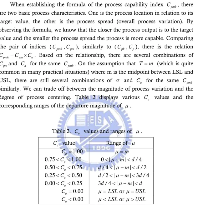
4.1 Simulation Layout Setting

When establishing the formula of the process capability index C_pmk, there are two basic process characteristics. One is the process location in relation to its target value, the other is the process spread (overall process variation). By observing the formula, we know that the closer the process output is to the target value and the smaller the process spread the process is more capable. Comparing the pair of indices (C_pmk ,C_pm), similarly to (C_pk ,C_p), there is the relation

pmk pm a

C =C ×C . Based on the relationship, there are several combinations of

pm

C and C_a for the same C_pmk. On the assumption that T m= (which is quite common in many practical situations) where m is the midpoint between LSL and USL, there are still several combinations of σ and C_a for the same C_pmk

similarly. We can trade off between the magnitude of process variation and the degree of process centering. Table 2 displays various values and the

corresponding ranges of the departure magnitude of

a

C

μ .

Table 2. C_a values and ranges of μ .

a C value Range of μ C =_a 1.00 μ =m 0.75<C_a <1.00 0 |< μ−m|<d/ 4 0.50<C_a <0.75 d/ 4 |< μ−m|<d/2 0.25<C_a <0.50 d/2 |< μ−m| 3 / 4< d 0.00<C_a <0.25 3 / 4 |d < μ−m|<d C =_a 0.00 μ =LSLor μ =USL C <_a 0.00 μ <LSL or μ >USL 14

(27)

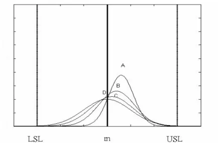
Figure 2. Four processes with C_pmk =1.00.

Table 3. Parameter values for two manufacturing suppliers used in the simulation study under C_pmk₁=C_pmk₂ =1.00.

Case# Cpmk1 μ1 C a1 σ1 Cpmk2 μ2 C a2 σ2 1 1 0.6 0.8000 0.5292 1 0.6 0.8000 0.5292 2 1 0.6 0.8000 0.5292 1 0.4 0.8667 0.7688 3 1 0.6 0.8000 0.5292 1 0.2 0.9333 0.9117 4 1 0.6 0.8000 0.5292 1 0 1.0000 1.0000 5 1 0.4 0.8667 0.7688 1 0.6 0.8000 0.5292 6 1 0.4 0.8667 0.7688 1 0.4 0.8667 0.7688 7 1 0.4 0.8667 0.7688 1 0.2 0.9333 0.9117 8 1 0.4 0.8667 0.7688 1 0 1.0000 1.0000 9 1 0.2 0.9333 0.9117 1 0.6 0.8000 0.5292 10 1 0.2 0.9333 0.9117 1 0.4 0.8667 0.7688 11 1 0.2 0.9333 0.9117 1 0.2 0.9333 0.9117 12 1 0.2 0.9333 0.9117 1 0 1.0000 1.0000 13 1 0 1.0000 1.0000 1 0.6 0.8000 0.5292 14 1 0 1.0000 1.0000 1 0.4 0.8667 0.7688 15 1 0 1.0000 1.0000 1 0.2 0.9333 0.9117 16 1 0 1.0000 1.0000 1 0 1.0000 1.0000

Figure 2 plots four processes with varied combinations of ( , )C_a σ with , LSL=-3, USL=3 and m=0, i.e.

1.00 pmk

C = ( , ) (0.8,0.5292)C_a σ = for process A,

σ =

( , ) (0.8667,0.7688)C_a for process B, ( , ) (0.9333,0.9117)C_a σ = for process C

(28)

and ( , ) (1,1)C_a σ = for process D (from right to left in plot). These four processes are equivalent according to C_pmk (i.e. C_pmk =1.00 for all four processes), and all have yields exceeding 99.73% but differ substantially with the magnitude of process variation and the degree of process centering. After setting the simulation environment, we make two investigations among the four bootstrap confidence limits to select a method which make our difference and ration testing more reliable. One is error probability analysis. We inspect the error probability from simulation results to know the magnitude of stability among four bootstrap methods. The other is selection power analysis. We choose a method with larger testing power by constructing the power curves. The sets of parameter values for two manufacturing suppliers used in the simulation study are given in Table 3. The selected parameters are chosen so as to investigate the performance of the methods for a wide range of index values and for both on-target and off-target processes. For each combination, a sample of size =100 was drawn with

B=3000 bootstrap replications, and the single simulation was then replicated

times. Further analysis will be shown in Sections 4.2 and 4.3.

n

3,000

N =

4.2 Error Probability Analysis

When deciding whether rejects the null hypothesis H or not, we might ₀

make a mistake. Generally speaking, hypothesis tests are usually evaluated and compared through their probabilities of making mistakes. In this section, we measure these error probabilities from four bootstrap methods to determine which methods of testing have smaller and stable error probabilities.

In our analysis of simulation, the error probability is the proportion of times that rejecting the null hypothesis H C₀: _pmk₁≥C_pmk₂ , while actually

0: pmk1 pmk2

H C ≥C is true. That is, we will calculate the proportion of times that the LCB of C_pmk₂ −C_pmk₁ is positive and the LCB of C_pmk₂/C_pmk₁ is larger than 1 when . While generating the simulation, a sample size

n=100 drawn with B=3000 bootstrap replications, the single simulation was

replicated N=3000 times and type I error

1 2 1.00

pmk pmk

C =C =

0.05

α = for each case given in Table 2. Usually, it is required that the probability of the error selection be less than a maximum value _{α , generally referred to as the}* _{α –condition. The frequency of}* error selection is a binomial random variable with N =3000 and . Thus, a 99% confidence interval for the error probability is

* _0.05 α = * * * 0.005 (1 )/ 0.05 2.576 (0.05 0.95)/3000 0.05 0.0103 Z N α ± × α −α = ± × × = ± . 16

(29)

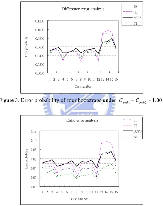
That is, one could be 99% confident that a “true 0.05% error probability” would have a proportion of range from 0.0397 to 0.0603. Thus, from the results of simulation for each case, we could depict confidence interval (0.0397, 0.0603). Figure 3 and Figure 4 show the error probability of four bootstrap methods for the difference and the ratio statistics with 16 combinations tabulated in Table 3, respectively.

Difference error analysis

0.0000 0.0200 0.0400 0.0600 0.0800 0.1000 SB PB BCPB 0.1200 1 2 3 4 5 6 7 8 9 10 11 12 13 14 15 16 Case number E rror proba bi lit y BT

Figure 3. Error probability of four bootstraps under C_pmk₁=C_pmk₂ =1.00.

Ratio error analysis

0.00 0.02 0.04 0.06 0.08 0.10 0.12 1 2 3 4 5 6 7 8 9 10 11 12 13 14 15 16 Case number E rr or p ro ba bi lity SB PB BCPB BT

Figure 4. Error probability of four bootstraps under C_pmk₁/C_pmk₂ = .001 . According to error probability analysis, it is shown that for the difference test, there are 7 combinations out of the 16 cases which were outside the interval (0.0397, 0.0610) for the SB, PB, BT methods. In contrast, 5 out of the 16 cases are beyond the interval for BCPB method. As for the ratio test, there are 11, 7 and 13

(30)

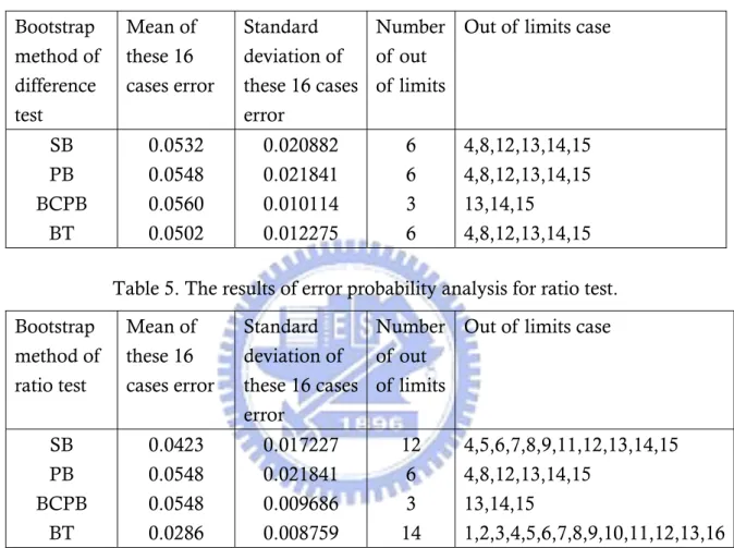
cases out of the 16 combinations outside the interval (0.0397, 0.0603) respectively. However, the BCPB method has only 5 out of 16 cases beyond these limits. Consequently, we know that the BCPB method has smaller and stable error probabilities for both difference and ratio test. Tables 4 and 5 show the results of error probability analysis for difference and ratio test.

Table 4. The results of error probability analysis for difference test. Bootstrap method of difference test Mean of these 16 cases error Standard deviation of these 16 cases error Number of out of limits

Out of limits case

SB 0.0532 0.020882 6 4,8,12,13,14,15

PB 0.0548 0.021841 6 4,8,12,13,14,15

BCPB 0.0560 0.010114 3 13,14,15

BT 0.0502 0.012275 6 4,8,12,13,14,15

Table 5. The results of error probability analysis for ratio test. Bootstrap method of ratio test Mean of these 16 cases error Standard deviation of these 16 cases error Number of out of limits

Out of limits case

SB 0.0423 0.017227 12 4,5,6,7,8,9,11,12,13,14,15

PB 0.0548 0.021841 6 4,8,12,13,14,15

BCPB 0.0548 0.009686 3 13,14,15

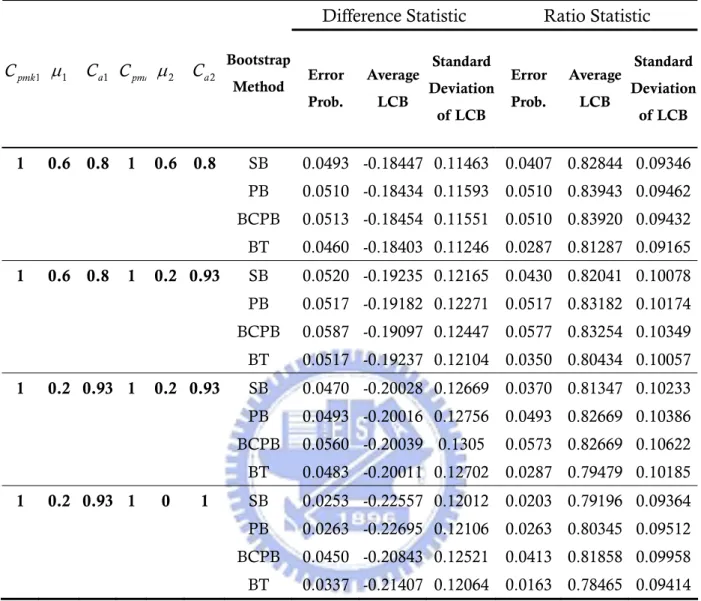
BT 0.0286 0.008759 14 1,2,3,4,5,6,7,8,9,10,11,12,13,16 In addition, an average lower bound and the standard deviation of the lower bound were calculated based on the N =3000 distinct trials. The complete data for error probability with 16 combinations of (C_a₁, )σ₁ and (C_a₂,σ₂) under

1

pmk

C =C_pmk₂=1 is tabulated in Appendix A. Error probability analysis information. Table 6 displays the particular four combinations of the average lower bound and the standard deviation of the lower bound for each of the four bootstrap confidence intervals.

(31)

Table 6. Simulation results of the four bootstrap methods for the difference and ratio statistics.

Difference Statistic Ratio Statistic

1 pmk C μ₁ C _a₁ C_pmk μ₂ C _a₂ Bootstrap Method Error Prob. Average LCB Standard Deviation of LCB Error Prob. Average LCB Standard Deviation of LCB 1 0.6 0.8 1 0.6 0.8 SB 0.0493 -0.18447 0.11463 0.0407 0.82844 0.09346 PB 0.0510 -0.18434 0.11593 0.0510 0.83943 0.09462 BCPB 0.0513 -0.18454 0.11551 0.0510 0.83920 0.09432 BT 0.0460 -0.18403 0.11246 0.0287 0.81287 0.09165 1 0.6 0.8 1 0.2 0.93 SB 0.0520 -0.19235 0.12165 0.0430 0.82041 0.10078 PB 0.0517 -0.19182 0.12271 0.0517 0.83182 0.10174 BCPB 0.0587 -0.19097 0.12447 0.0577 0.83254 0.10349 BT 0.0517 -0.19237 0.12104 0.0350 0.80434 0.10057 1 0.2 0.93 1 0.2 0.93 SB 0.0470 -0.20028 0.12669 0.0370 0.81347 0.10233 PB 0.0493 -0.20016 0.12756 0.0493 0.82669 0.10386 BCPB 0.0560 -0.20039 0.1305 0.0573 0.82669 0.10622 BT 0.0483 -0.20011 0.12702 0.0287 0.79479 0.10185 1 0.2 0.93 1 0 1 SB 0.0253 -0.22557 0.12012 0.0203 0.79196 0.09364 PB 0.0263 -0.22695 0.12106 0.0263 0.80345 0.09512 BCPB 0.0450 -0.20843 0.12521 0.0413 0.81858 0.09958 BT 0.0337 -0.21407 0.12064 0.0163 0.78465 0.09414

4.3. Selection Power Analysis

Power is broadly defined as the probability that a statistical significance test will reject the null hypothesis for a specified value of an alternative hypothesis. Another way to define it is the ability of a test to detect an effect, given that the effect actually exists. If a study that is inefficiently precise or lacks power to reject a false null hypothesis, it will waste time and money in practical situation.

Therefore, in this section, we conduct selection power analysis to compare the performance of those four bootstrap methods. It is essential to apply a method which is efficiently precise and with power in hypothesis testing. Further simulations of selection power analysis are implemented with sample sizes

=10(10)200 for and

n C_pmk₁ =1.00 C_pmk₂ =1.05(0.05)1.50. The selection power

computes the probability of rejecting the null hypothesis H C0: pmk1 ≥Cpmk2 while

(32)

actually H C1: pmk1 <Cpmk2 is true. For the difference statistic, the selection power computes the proportion of times that the LCB of C_pmk₂−C_pmk₁ is positive in the simulation. Similarly, for the ratio statistic, the selection power computes the proportion of times that the LCB of C_pmk₂/C_pmk₁ is larger than 1. Figures 5-6 are the power curves of the four bootstrap methods for the difference and ratio statistic for on-target process with sample size = 10(10)200, ,

,

n C_pmk₁=1.00

2 1.50

pmk

C = μ₁= , 0 μ₂ = , respectively. 0

Cpmk1=1.00 Cpmk2=1.50 Diference Power Curve

0 0.2 0.4 0.6 0.8 1 0 20 40 60 80 100 120 140 160 180 200 Sample Size Se le ct io n Po w er SB PB BCPB BT

Figure 5. The selection power for the difference statistic for on-target process with sample size n=10(10)200,

, 1 1

pmk

C = C_pmk₂=1.50, μ₁ =μ₂ =0 .

Cpmk1=1.00 Cpmk2=1.50 Ratio Power Curve

0 0.2 0.4 0.6 0.8 1 0 20 40 60 80 100 120 140 160 180 200 Sample Size Se le ctio n P ow er SB PB BCPB BT

Figure 6. The selection power for the ratio statistic for on-target process with sample size n =10(10)200, C_pmk₁ =1,

2

pmk

C =1.50, μ₁ =μ₂ =0 .

Similarly, Figures 7-8 are the power curves of the four bootstrap methods for the difference and ratio statistic for off-target process with sample size = 10(10)200,

, , n 1 1.00 pmk C = C_pmk₂ =1.50 μ₁=0.4, μ₂ =0.4, respectively.

Cpmk1=1.00 Cpmk2=1.50 Difference Power Curve

0 0.2 0.4 0.6 0.8 1 0 20 40 60 80 100 120 140 160 180 200 Sample Size S ele ctio n Po w er SB PB BCPB BT

Figure 7. The selection power for the difference statistic for off-target process with sample size n=10(10)200,

, 1 1

pmk

C = C_pmk₂=1.50, μ₁ =μ₂ =0.4 .

Cpmk1=1.00 Cpmk2=1.50 Ratio Power Curve

0 0.2 0.4 0.6 0.8 1 0 20 40 60 80 100 120 140 160 180 200 Sample Size S ele ctio n P ow er SB PB BCPB BT

Figure 8. The selection power for the ratio statistic for off-target process with sample size n = 10(10)200,

1 1

pmk

C = , C_pmk₂=1.50, μ₁ =μ₂ =0.4 .

(33)

According to Figures 5-8, it is shown that the PB and BCPB methods have larger selection power with fixed sample size in contrast with the SB and BT methods. In other words, we only need smaller required sample size for the PB and BCPB methods when conducting hypothesis test. By evaluating both error probability and selection power, the BCPB method has more stable error probability and larger selection power with fixed sample size. Consequently, we suggest that the BCPB method among four bootstrap methods is the better approach for further analysis. Besides Figures 5-8, the complete data and power curves are shown in Appendix B.

(34)

5. Supplier Selection Based on BCPB Method

5.1 Sample Size Determination with Designated Selection Power

It is a practical and important issue to determine an appropriate sample size for supplier selection problem in manufacturing industries. A study that lacks of power to reject a false null hypothesis is a waste of time and money. On the other hand, an investigation collects too many samples or has too much power to reject Ho is also wasteful for manufacturing. Thus, the requirement of appropriate sample size with designed selection power should be determined carefully before conducting the hypothesis test.

According to error probability and selection power, it has been suggested that the best of those four bootstrap methods in our study is the BCPB method. Thus, the simulation technique was applied to investigate the BCPB method with

=3,000 bootstrap replications, and the single simulation was then replicated

B

N =3,000 times. For practical application and engineers’ convenience, we

calculate the requirement of sample size for difference and ratio hypothesis test by using MATLAB program. For both of the two tests, it has been investigated with

1.00 and 1.33 for supplier I and 1

pmk

C = C_pmk₂ =1.15(0.05)1.50 and 1.48(0.05)1.83

for supplier II. The designated selection power = 0.90, 0.95, 0.975 and 0.99 which computes the probability of rejecting the null hypothesis H C0: pmk1 ≥Cpmk2 while actually H C1: pmk1 <Cpmk2 is true. Tables 7-10 display the sample size required of the BCPB method for the difference and ratio statistic with various selection powers.

Table 7. Sample size required of BCPB method for the difference statistics under α =0.05 , with power = 0.90, 0.95, 0.975, 0.99, ,

. Cpmk1 =1.00 2 1.15(0.05)1.50 pmk C = 1 pmk C _{1 1 1 1 1 1 1 1} 2 pmk C _{1.15 1.2 1.25} _{1.3 1.35} _{1.4 1.45 1.5} 90% 505 288 189 140 107 83 69 58 95% 627 365 246 174 138 107 87 74 97.50% 745 430 284 207 164 125 104 87 99% 918 538 369 263 200 158 130 115 22

(35)

Table 8. Sample size required of BCPB method for the ratio statistics under 0.05 α= , with power = 0.90, 0.95, 0.975, 0.99, , . 1 1.00 pmk C = 2 1.15(0.05)1.50 pmk C = 1 pmk C _{1 1 1 1 1 1 1 1} 2 pmk C _{1.15 1.2 1.25} _{1.3 1.35} _{1.4 1.45 1.5} 90% 504 293 199 143 109 83 72 58 95% 624 378 241 176 135 110 89 73 97.50% 765 446 291 214 156 127 105 88 99% 945 531 364 248 203 157 128 108

Table 9. Sample size required of BCPB method for the difference statistics under α =0.05 , with power = 0.90, 0.95, 0.975, 0.99, ,

. 1 1.33 pmk C = 2 1.48(0.05)1.83 pmk C = 1 pmk C _{1.33 1.33 1.33 1.33 1.33 1.33 1.33 1.33} 2 pmk C _{1.48 1.53 1.58 1.63 1.68 1.73 1.78 1.83} 90% 820 465 313 226 171 136 109 91 95% 1027 582 397 275 212 168 136 113 97.50% 1215 713 475 332 250 196 159 137 99% 1485 863 580 413 307 248 198 165

Table 10. Sample size required of BCPB method for the ratio statistics under 0.05 α= , with power = 0.90, 0.95, 0.975, 0.99, , . 1 1.33 pmk C = 2 1.48(0.05)1.83 pmk C = 1 pmk C _{1.33 1.33 1.33 1.33 1.33 1.33 1.33 1.33} 2 pmk C _{1.48 1.53 1.58 1.63 1.68 1.73 1.78 1.83} 90% 815 469 315 228 175 136 111 91 95% 1059 582 386 275 213 169 140 116 97.50% 1262 732 467 338 270 212 167 137 99% 1912 1032 692 538 420 362 198 166

For the convenience of observation, Figures 9-12 depict sample size curves based on the four sample size tables, respectively.

依據製程能力指標 Cpmk 應用複式抽樣方法於供應商選擇

國立交通大學

工業工程與管理學系

碩士論文

依據製程能力指標

C

應用複式抽樣方法於

供應商選擇

Bootstrap Approach for Supplier Selection Based on

Process Capability Index

C

研 究 生：邱勝亮

指導教授：彭文理 博士

吳建瑋 博士

依據製程能力指標

C

應用複式抽樣方法於

供應商選擇

Bootstrap Approach for Supplier Selection Based on

Process Capability Index

C

國 立 交 通 大 學

工 業 工 程 與 管 理 學 系

碩 士 論 文

A Thesis

Submitted to Department of Industrial Engineering and Management

College of Management

National Chiao Tung University

in partial Fulfillment of the Requirements

for the Degree of

Master

in

Industrial Engineering

May 2007

Hsinchu, Taiwan, Republic of China

依據製程能力指標

C

應用複式抽樣方法於

供應商選擇

研究生：邱勝亮 指導教授：彭文理 博士

吳建瑋 博士

國立交通大學工業工程與管理學系碩士班

摘要

Bootstrap Approach for Supplier Selection Based

on Process Capability Index

C

Student: Sheng-Liang Chiu

Advisor：

.

Dr. W. L. Pearn

Dr. Chien-Wei Wu

Department of Industrial Engineering and Management

National Chiao Tung University

Abstract

誌謝

這篇碩士論文的完成，首先要感謝我的指導教授彭老師，老師在做

研究上一向要求嚴謹，也因為這樣的態度，才能有顯著的學術成就。

在對待學生上，除了對我們論文的要求外，寶貴的人生經驗談與做事、

做學問的態度，是我兩年內最大的收穫。

此外，建瑋學長，感謝給了我許多論文上的建議，還不辭辛苦的

往返台中，新竹兩地，鍾老師在口試上也幫了我很多的忙。博班的學

長、學姊們，MB517、519、516 的研究室夥伴們，很高興和大家一起相

處，使我這兩年過得多采多姿。

最後，謝謝我的爸爸、媽媽，讓我可以在舒適、安逸的環境學習，

希望他們保持身體健康，天天快樂。

Contents

Abstract (Chinese)

Abstract

誌謝

Contents

List of Table

List of Figure

Notations

1. Introduction

2. Literature Review

3. Selection Method

4. Performance Comparison of Four Bootstrap Methods

5. Supplier Selection Based on BCPB Method

6. Application

Example

研究生：邱勝亮

指導教授：彭文理博士

吳建瑋博士

國立交通大學

工業工程與管理學系

碩士論文

研究生：邱勝亮指導教授：彭文理博士

吳建瑋博士

_∫