FREE-VIBRATION OF A THIN SPHERICAL-SHELL CONTAINING A COMPRESSIBLE FLUID

Free vibration of a thin spherical shell containing

a compressible fluid

Mingsian R. Bai and Kuorung Wu

Department of Mechanical Engineering, National Chiao Tung University, Hsin Chu 30050, Taiwan, Republic of China

(Received 28 April 1993; revised 22 November 1993; accepted 18 January 1994)

Free vibration of a thin spherical shell filled with a compressible fluid is investigated. The interactions at the interface between the elastic structure and the compressible fluid are taken into account. The objective of this study is to develop a hybrid .numerical technique for the free vibration analysis of sound-structure interaction problems. The boundary element method is employed for modeling the acoustic disturbances in the cavity, while the finite element method is used for modeling the structural dynamics of the shell. The formulations are then combined into a coupled numerical scheme for the total pressure-displacement field. Natural frequencies and mode shapes are calculated by using the singular value decomposition algorithm. Physical insights into the resonance phenomena associated with sound-structure interactions are derived .from the comparison between the results of the thin spherical shell, with and without the fluid loading effect.

PACS numbers: 43.40.Ey

INTRODUCTION

For an elastic structure filled with a compressible fluid,

interactions exist between the acoustic field of the fluid and

the vibration field of the structure. In most cases, the dy- namic response of a structure in contact with a fluid can be determined as if the structure were vibrating in vacuo be- cause the radiation loading exerted by the fluid is generally small enough to have a negligible effect on the structural vibrations. Radiation loading significantly ... mooroes the '- - mo- tion of a structure only under exceptional circumstances, e.g., when a volume of air is confined in a small enclosure, when the structure is relatively light, or when an elastic structure is submerged in a heavy fluid. On these occasions,

the elastic structure and the acoustical field cannot be

treated as uncoupled systems and must be solved simulta- neously.

There has been ongoing research on the subject of sound-structure interactions. To name a few, the sound- structure interaction problem was explored by Faran in 1951 who used the method of separation of variables to derive closed form solutions for acoustic fields scattered by

elastic

solid

cylinders

and spheres.

• Then,

Junger

used

an

analytical approach to solve acoustic fields scattered by

thin elastic

shells.

2 Instead

of analytical

approaches,

Chen

and Schweikert applied numerical methods to analyze fluid-structure interactions for arbitrarily shaped bodies

submerged

in an infinite

medium.

3 In 1977,

Zienkiewicz,

Kelly, and Bettess proposed a finite element method

(FEM)-based

formulation

for coupled

systems.

4 Then,

Wilton solved an exterior fluid-structure interaction prob- lem by coupling the boundary element method (BEM)

and the FEM.

• More recently,

an analysis

was

presented

by Wu for analyzing radiation and scattering problems as-

sociated

with submerged

elastic

axisymmetric

bodies.

6

category of exterior problems when the structures are sub- merged in fluids. This does not preclude the importance of interior sound-structure interaction problems, where the structures may contain fluids in their interiors. There are many situations in which the interior problems of sound- structure interactions may be of importance, such as ram- jet engines, nuclear reactors, and pressure vessels. Al- though the literature concerning the interior problems of sound-structure interactions is not as ample as that of the exterior counterpart, similar numerical techniques can still be applied to calculate the total response of a containing elastic structure. Of particular interest in this study is the development of a hybrid numerical method for the free vibration analysis of structures filled with compressible flu- ids. While the numerical technique is developed in a rather general form, a thin spherical shell container is chosen in the simulation to verify the algorithm not only because it interacts more strongly with the contained fluid compared with the thick shell, but also because its analytical solution is more tractable than the other odd-shaped structures. Nevertheless, the numerical simulation is conducted with- out taking the advantages of symmetry. The method de- veloped thus can be applied to problems of arbitrary ge- ometries where analytical solutions are in general not

available.

The objective of this research is twofold: first, to dem- onstrate the implementation of the coupled FEM-BEM technique; and, second, to explore the sound-structure in-

teraction behavior via an extensive numerical simulation.

The free vibration analysis has three steps. First, the acous- tic field enclosed by a rigid spherical boundary is analyzed by BEM. Next, the free vibration of a thin spherical shell in vacuo is analyzed by FEM. Finally, the free vibration of the containing thin spherical shell subjected to loading ef- fects is analyzed by the coupled BEM-FEM technique. An algorithm based on singular value decomposition (SVD) is

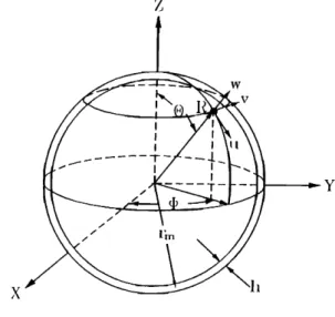
x.: fiel(! l•oii•l

FIG. 1. Schematic diagram for an interior boundary value problem of the

acoustic field in an enclosure.

W

V

developed

for efficiently

searching

for the natural

frequen-

cies and mode

shapes

of the coupled

system.

Physical

in-

sights

are derived

from the results

of the spherical

shell

with and without the fluid loading.

I. ANALYSIS OF THE ACOUSTICAL SYSTEM

From the theory of linear acoustics, a monochromatic sound field in an inviscid and compressible fluid is de-

scribed

by the Helmholtz

equation

7

(V2

+ k2)p(x)=0,

( 1 )

where

k=co/c is the wave number

(co

and c are, respec-

tively, the angular frequency and the speed of sound). The radius of the spherical enclosure is a. The interior acoustic field has the general solution

p(x,n,m ) = [Anm cos(m•b)

-3- Bnm sin(mr) ]P•n (cos O)jn(kr), (2) where A nm and Bnm are arbitrary constants to be deter- mined by boundary conditions, P•n is the associated Le- gendre polynomial (rn<n), and Jn is the spherical Bessel

function of the first kind of order n.

Alternatively,

the solution

of the interior boundary

value problem

of the acoustic

field of Fig. 1 can be ex-

pressed as the Kirchhoff-Helmholtz integral

a(xp)p(xp)

=

G(xp,Xq)

•nqp(Xq)

a

)

--p(Xq)

•q G(Xp,Xq)

dS,

(3)

1, x•,• V,

a(x•,)= fl(xp)/4rr, x•,•S

0, x• V'

[q•(xp) is the solid angle at the point xp],

8

G(xp,Xq)=exp(ikr)/4•r

is the free-space

Green's

func-

tion,

the position

vectors

xp and

Xq

denote

the field

point

and the source point, respectively, the distance

r=lxp--Xq[,

and the directional

directive

O/Onqmnq.

V

FIG. 2. The thin spherical shell and spherical coordinates.

with n e being

the outward

normal

to the surface

S.

With the field point taken to the boundary

S, Eq. (3)

becomes a boundary integral equation, which can further

be discretized into a matrix form 9

AP--BPn=0, (4)

where

P is the acoustic

pressure

vector

and Pn is the acous-

tic pressure gradient vector. Here, Eq. (4) constitutes the main equation for the acoustical subsystem. For some sub-

tle points

involved

in the numerical

implementation,

such

as fictitious

frequencies,

nonsmooth

boundaries,

and singu-

lar elements,

one may consult

the related

literature

(e.g.,

Ref. 9).

II. ANALYSIS OF THE STRUCTURAL SYSTEM

A. Analytical solution of the thin spherical shell in

vacuo

Consider a thin spherical shell of thickness h and ra- dius r m (h •rm), as shown in Fig. 2, with the material properties: the mass density Ps, the Young's modulus E,

and Poisson's ratio v. From the Love-Kirchhoff

theory

lø-12

of thin

shells,

the simplified

shell

equations

for

monochromatic motions based on axisymmetry are

Luuu

+ Luww+

fl2u

= 0,

(5)

Lwuu

+ Lwww

+ l•2w

= --q( 1 -- v 2) r2m/Eh,

(6)

2 2

where the nondimensional

frequency

1•2=co

r2m/C•,

%

= [E/( 1 -- v 2) pj 1/2

is the phase

velocity

of compressible

waves, q is the normal stress acting on the middle surface,

and the differential

operators

Luu, Luw, Lwu,

and Lww

are

defined as

Luu=(l_+_y2)((l_r12)1/2

•2 (1-T]2)1/2-+-(1-¾)

d2

)

, (7)

tuw=(1--V:•)

1/:•

[72(1--v)

-- (1

+v)l•-•+y

2

• V ,

(8)

d •2

1/2

Lwu

=-- [y2(1--•)--(l+•)]•(1--

)

-3-

•2V•

•-• ( 1

-- T]2)

1/2

,

(9)

2--2(1+v),

(10)

with

•-- 12•m,

V•--sin

0 •0 sin

0 •sin

2

0 O•

•'

(11)

:

d

d

v•=• (•-•:) d•'

The free vibration of the spherical shell can be analyzed in terms of P.(•), the Legendre polynomial of the first kind

of order n:

u(•/)=

_.=0

• Un(1--•12)

1/2dPn(*l)

_{d•/ '}

₍₁₂₎

w(•l)- • W.P.(•I).

(13)

n=0

Hence, the expansion coefficients U. and W. must satisfy

the relations

[f•2-- (1 + y2) (¾+,• n-- 1)JUn

- [•(v+z•-

•) + ( • +v) ] w•=o,

(•4)

A.[f(v+A.-

1)+(1 +v)JUn

-- [•2--2( 1 +v)--•Xn(v+X n-- 1 )] Wn=O,

(15)

where A. n (n + 1 ). The determinant of the coe•cients must vanish for nontrivial solutions of the unknowns Un and W.. This leads to the frequency equation

•4-[ 1 + 3v+A.+d(A.

1)(•. 1 +v) ]•2

- (•. 2) (1-•) + d(•.- 2) [ (•. 1)2-•] =0.

(16) Each mode associated with an index n > 0 corresponds to two distinct branches of resonant frequencies. However, for n=0 corresponding to what is called the breathing mode, only one real frequency exists. On the other hand, for nonaxisymmetric torsional modes, another frequency equation reads

n2-n2•=o,

(•7)

where

•. = [• ( n + 2 ) ( n - 1 ) ( 1 + • ) ( 1 - v ) ]•/2.

B. The numerical method (FEM)

Standard FEM formulation of an elastic structure

yields

the matrix

equation

for harmonic

motions,

13

(K+koC--w2M)U=R, (18)

where K, C, and M are, respectively, the stiffness matrix, damping matrix, and mass matrix; R is the external force vector; and U is the displacement vector. The matrices K,

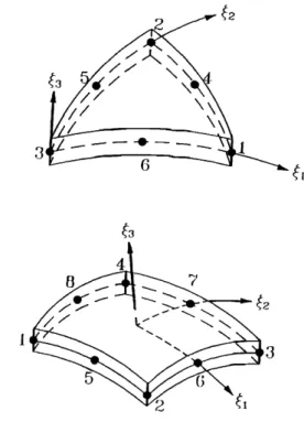
FIG. 3. The six-node and eight-node degenerate shell elements.

C, M, and R are assembled from the matrix for the element e as 13

K=

ZK

(e)--

•e

fIA

•tE•dV'

(19,

C

= Z c(e)---

•e

f [l.L•tl•

dV,

(20,

M--

•e

M(e)=

•e

L ps•tX•

dV,

and

R= Z R(e)

•tb dV+

•,Itq

dS+ Z Fi,

= Z e)

(e)

in which B is the strain-displacement matrix, E is the stress-strain matrix, N is the shape function matrix, b is the body force vector, q is the traction vector, F i is the con- centrated force vector, and Ps and p are the mass density and damping factor of the structure, respectively.

In principle, a three-dimensional elasticity problem can be modeled by solid elements that are, unfortunately,

not suited for the thin shell considered here because of its

exceedingly

large

aspect

ratios.

TM

In fact, spherical

shell

elements happen to be among the structural elements the most difficult clements to &sign in implementing FEM codes. Special types of six- and eight-node degenerate curved shell elements in Fig. 3 are thereby employed for the analysis of the thin spherical shell. The details can be

found in Refs. 15 and 16.

III. FREE VIBRATION ANALYSIS OF THE COUPLED SYSTEM

A. Analytical solution of the coupled system

A modal matching method is used for obtaining the analytical solution of the coupled fluid-shell system. Con- sider the forced vibration of the thin spherical shell sub- jected to a harmonic excitation pressure q=f(r/)exp(kot),

which can be expanded in terms of the Legendre polyno- mials Pn (r/) as

f(r/)= • fnPn(•7).

(23)

n=0

Substituting Eq. (23) into the equations of motion (5) and (6) gives

[112--(

1 q- y2) (vq-Xn--

1)]Un

-- [72(v+•n -- 1) + ( 1 +v) ] Wn=0,

(24)

An

[72(vq-An

- 1 )+ ( 1 +v)] Un

--[112--2( 1 +v)--y2•n(v+• n-- 1) ] Wn

= [ (1--v2)•/Eh ]f n .

(25)

For the sound-structure interaction problem, the excita- tion pressure q should be replaced by the negative of inter- face acoustic pressure --Pi:

irozWl=,

(26)

n=0

where

zn = ip•jn (kri)/j • (kri) denotes

the interface

acous-

tic modal impedance. Direct comparison of Eqs. (23) and

(26) reveals

that fn = pjcwjn(kri)/j}(kri)Wn. Thus the

frequency equation turns out to be

( l p•c

jn(kr')

)114

-(

1

p•c

Jn(kri)

)

+

(1 +y2) (gn_ 1 +v) 112

-- (gn--2) ( 1--v 2) +y2(gn-- 2) [ (gn-- 1)2--v

2 ] =0.

with the solutions of the shell in vacuo as the initial

guesses.

B. The interface conditions

In order to couple the matrix equations of the acous- tical and structural subsystems, the compatibility at the interface must be considered. First, the surface velocity of the structure and the particle velocity of the fluid at the interface along the normal direction must be equal. Sec- ond, the normal stress of the elastic structure must equal

the acoustic pressure at the interface. The compatibility of velocity and stress in tangential directions at the interface is not imposed because the fluid is assumed to be inviscid.

If the interaction force is treated as the excitation to

the structure, Eq. (18) can be modified into

( K q- icoC--co2M)

U = Rex

t -i- Rint,

(28)

where Rex t denotes the externally applied force vector and Rin t denotes an equivalent acoustic force vector acting on

the surface of the structure.

The major step of coupling the acoustical and struc- tural subsystems in Eqs. (4) and (28) is accomplished through the use of two coupling matrices L and T (Refs. 5

and 17):

Rin t = LP ( 29 )

and

Pn = -- ipffoTU.

(30)

The former represents the acoustic pressure and the latter represents the pressure gradient (or, equivalently, the par- ticle velocity) obtained from the Euler's equation along the

normal direction at the interface.

C. The coupled system matrices

As mentioned previously, when the interaction be- tween the fluid and the structure is not negligible, the dy- namic characteristics of the coupled system must be solved simultaneously. Various approaches can be utilized to form the coupled system equations. One may either substitute the acoustical system equations into the structural system equations (termed the structural variable approach), sub- stitute the structural system equations into the acoustical system equations (termed the acoustical variable ap- proach), or assemble both subsystem equations into a com- plete set of system equations (termed the mixed variable approach). In this study, the structural variable approach is adopted because it is less computationally expensive than the others. From Eqs. (4), (29), and (30), the interaction

force vector can be written as

Rin

t = -- ipffoLA-

1BTU.

Then, substituting Eq. (31 ) into (28) leads to

(31)

(K+iooC--co2M+ipffoLA-•BT)U=Rext.

(32)

In Eq. (31), let ipffoLA-iBT=icoRa--co2Rm

(R

a and

R m

are the added damping and mass matrices, respectively, which may alter the frequency response of the coupled

systemS).

A coupled

system

equation

in terms

of structural

displacements is then obtained:

[K +ko(C+ Rd) --co2(M

+ Rm)

]U=Rext.

[K-co2(Mq-Rm)

]U=0.

ß • Y Y Y

(a) (c)

•x

(b)

•x

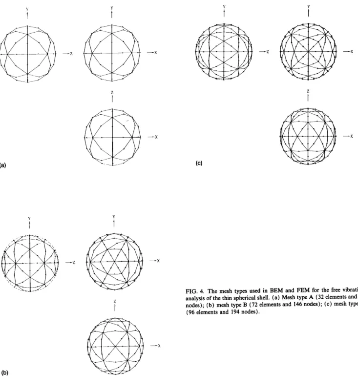
FIG. 4. The mesh types used in BEM and FEM for the free vibration analysis of the thin spherical shell. (a) Mesh type A (32 elements and 66 nodes)' (b) mesh type B (72 elements and 146 nodes)' (c) mesh type C

(96 elements and 194 nodes).

Eq. (34) is a nonstandard

eigenvalue

problem

since

the

added mass matrix a m is a function of frequency D. The numerical scheme of searching for natural frequencies and mode shapes

Searching

for natural

frequencies

and mode

shapes

of

the coupled

sound-structure

system

amounts

to solving

the

eigenvalue

problem

represented

by Eq. (34). Frequencies

that render

the system

matrix singular

correspond

to the

eigenvalues

and

the nontrivial

solutions

correspond

to the

eigenvectors.

This eigenvalue

problem

of the coupled

sys-

tem differs from that of the structure in vacuo in that the

latter is a standard

eigenvalue

problem

Ax=,;tx, but the

former is not. For such a nonstandard eigenvalue problem,

the eigenvalues

are embedded

in the coefficient

matrices,

which

obviously

poses

difficulties

for ordinary

numerical

eigenvalue

solvers.

It is thus

desirable

to develop

a numer-

ical scheme

for the eigenvalue

analysis

of the sound-

structure

interaction

problem.

To this end,

two approaches

termed the method of determinant search and the method

of singular

value

decomposition

(SVD) are employed.

Let •(to)=[K--w2(M+Rm)] ß In the method

of de-

terminant search, one seeks to determine the eigenvalues

by incrementally

varying

the angular

frequency

to such

that the matrix D(to) becomes singular. This amounts to finding the angular frequency toe, e= 1,2,..., such that the determinant of D(to) vanishes. In practical implementa- tion, one can locate only the local minima of the determi- nant of D(to) for the eigenvalues because it is virtually impossible for D(to) to become numerically singular.

On the other hand, the method of SYD involves searching for the frequencies at which the minimum sin- gular value of the coefficient matrix reaches local minima. From linear algebra, the following decomposition of the matrix fi exists: 18

(35)

Here h denotes the Hermitian transpose, U and V are both NX N unitary matrices and are composed of N orthogonal column vectors ui and vi, and ß is a diagonal matrix:

!tri•0, i--j, tri's

are singular

values,

•ij= {0, otherwise.

If the matrix D is almost singular, then the last one or more singular values must be nearly zero. In order to ex- tract the eigenvalues toe, the angular frequency to is incre- mentally varied with the step size Ato. Each D(to) corre- sponding to different to is processed by the SVD algorithm and the minimal singular value tr n is compared with those obtained from the other iterations. If the minimal singular value tr n of the matrix D(to) reaches a local minimum with respect to the angular frequency to, then this angular fre- quency to is accepted as a desired eigenvalue (although the minimal singular value tr n may not be numerically zero). Once a possible interval of eigenvalues has been located,

optimization

schemes

such

as the Golden

section

search

19

can then be used to efficiently calculate more accurate ei- genvalues. Parallel to searching for eigenvalues, the eigen- vectors (or mode shapes) are obtained without additional effort. This is accomplished by a simple observation: Whenever a singular value % vanishes, the fight singular vector vi of D can be regarded as a legitimate eigenvector. This feature of SVD for finding linearly independent eigen- vectors is particularly attractive when there are repeated eigenvalues (which are frequently encountered in problems of high degree of symmetry).

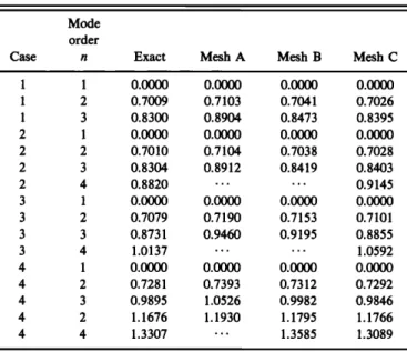
TABLE I. Nondimensional natural frequencies I1--tOrm/C p of the thin spherical shell. (E--1.9X10 TM Pa, ¾--0.3, ps--7700 kg/m3; case 1:

h/rm=O.002; case 2: h/rm-O.01' case 3: h/rm=O. 1; case 4: h/rm=0.2.)

Mode

order

Case n Exact Mesh A Mesh B Mesh C

1 1 0.0000 0.0000 0.0000 0.0000 1 2 0.7009 0.7103 0.7041 0.7026 1 3 0.8300 0.8904 0.8473 0.8395 2 1 0.0000 0.0000 0.0000 0.0000 2 2 0.7010 0.7104 0.7038 0.7028 2 3 0.8304 0.8912 0.8419 0.8403 2 4 0.8820 ... 0.9145 3 1 0.0000 0.0000 0.0000 0.0000 3 2 0.7079 0.7190 0.7153 0.7101 3 3 0.8731 0.9460 0.9195 0.8855 3 4 1.0137 ... 1.0592 4 1 0.0000 0.0000 0.0000 0.0000 4 2 0.7281 0.7393 0.7312 0.7292 4 3 0.9895 1.0526 0.9982 0.9846 4 2 1.1676 1.1930 1.1795 1.1766 4 4 1.3307 '" 1.3585 1.3089

0.002, 0.01, 0.1, and 0.2. In considering numerical accu- racy as well as efficiency, numerical integration is carried out by using 2 X 2 Gauss points in the middle surface (an increased number of Gauss points, say, 3 X 3, may result in an overstiff system, which is called the shell locking

phenomenonl3).

Table I summarizes

the analytical

solu-

tions and the numerical results of the natural frequencies

for the several lowest modes. It is evident that the error of the numerical results is reduced as the number of elements

is increased. In addition, case 4 shows the natural frequen- cies of some torsional modes which can only be obtained by sufficiently fine meshes (i.e., meshes B and C).

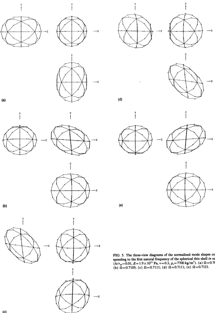
The mode shapes of the first natural mode (with mul- tiplicity 5) of the spherical shell with the thickness to ra- dius ratio 0.01 calculated by using SVD (based on the mesh type A) are shown in Fig. 5. It is observed from these figures that the spherical shell is deformed into a spheroi- dal shell. These calculated mode shapes will be compared with those of the containing thin spherical shell in the discussion of the coupled sound-structure system.

IV. NUMERICAL INVESTIGATIONS

A numerical simulation is undertaken to verify the developed BEM-FEM technique. The dynamic character- istics between the thin spherical shells (with and without the fluid loading) are compared. Quadratic triangular ele-

ments are used to construct the mesh on the interface for

both the BEM and FEM. The mesh configurations of the BEM and FEM used in the simulation are shown in Fig. 4. The mesh types A, B, and C consist of 32, 72, and 96 elements and 66, 146, and 194 nodes, respectively. A. The spherical shell in vacuo

The free vibration of the thin spherical shell is ana- lyzed by the FEM. The effects of the thickness to radius ratio and type of mesh on the results are investigated in the

simulation. The thickness to radius ratios selected are

B. The spherical shell filled with a compressible fluid In this section, a free vibration analysis is presented to explore the contributing factors that affect the interactions

between the structure and the fluid.

First, the effect of thickness to radius ratio is investi-

gated. Consider a spherical shell made of steel and filled with water. The material properties and physical dimen-

sions

are rm--1.0

m, E= 1.9X 10

TM

Pa, v=0.3, ps=7700.0

kg/m

3, p f--1000.0

kg/m

3, and c= 1460.0

m/s. Three

kinds of thickness to radius ratios, h/rm=O.002, 0.01, and 0.2, are chosen for the numerical simulation. The results of the minimum singular values are plotted against the non-

dimensional

natural

frequency/1

=torm/%

in Fig. 6 for the

case of thickness to radius ratio 0.01. The natural frequen- cies of the first two natural modes of the shell, with and without the fluid loading, obtained independently from the

Y Y Y Y z z --•x (a) (d) •x Y Y Y Y z z •x (b) (e) •x Y Y (c)

FIG. 5. The three-view diagrams of the normalized mode shapes corre- sponding to the first natural frequency of the spherical thin shell in vacuo (h/rm=O.01, E= 1.9X l0 ll Pa, v--0.3, ps--7700 kg/m3). (a) •--0.7072;

(b) 1•--0.7105; (c) 1•--0.7111; (d) 1•--0.7111; (e) 1•--0.7121.

2.0E+6

• 1.5E+6

'• I.OE+6

i

I

0.0 0.1 0.•2 0.3 0.4

0.5

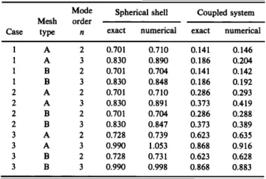
TABLE II. Nondimensional natural frequencies •--OJrm/C.p of the thin containing spherical shell filled with water. (E=l.9X10 ll Pa, v=0.3,

ps=7700 kg?m 3, pf--1000 kg/m 3, c= 1460 m/s; case 1:h/rm=O.002;

case 2:h?rm=O.01; case 3: h?rm=0.2.)

Mode Spherical shell Coupled system Mesh order

Case type n exact numerical exact numerical

1 A 2 0.701 0.710 0.141 0.146 1 A 3 0.830 0.890 0.186 0.204 1 B 2 0.701 0.704 0.141 0.142 1 B 3 0.830 0.848 0.186 0.192 2 A 2 0.701 0.710 0.286 0.293 2 A 3 0.830 0.891 0.373 0.419 2 B 2 0.701 0.704 0.286 0.288 2 B 3 0.830 0.847 0.373 0.389 3 A 2 0.728 0.739 0.623 0.635 3 A 3 0.990 1.053 0.868 0.916 3 B 2 0.728 0.731 0.623 0.628 3 B 3 0.990 0.998 0.868 0.883

• 6.0E+5

'• 4.0E+5

FIG. 6. Minimum singular values plotted against the nondimensional frequency f• of the containing spherical thin shell (h/rm=O.01,

E-- 1.9X 10 • Pa, v--0.3, ps--7700 kg/m 3, pf= 1000 kg/m 3, c= 1460

m/s). (a) Mesh type A; (b) mesh type B.

analytical and numerical methods are compared in Table II. From the results, it is observed that the natural frequen- cies of the coupled system are lower than those of the structure in vacuo. Significant decrease of natural frequen- cies occurs for very thin shell structures that interact strongly with the contained fluids. This can be attributed to the added mass effect resulting from the radiation reac-

tance of the interior acoustic field.

The multiplicity of an eigenvalue of the coupled sys- tem can be determined by the number of singular values which are closer to zero in comparison with the others. In some cases, repeated eigenvalues spill over within a small

interval of wave numbers. Great care has to be taken in

determining the multiplicity of eigenvalues which may be the sum of the multiplicities of several proximate local minima within a small interval located by SVD. Suffi- ciently small step size of wave number is generally required for finding a complete set of multiple eigenvalues. For ex-

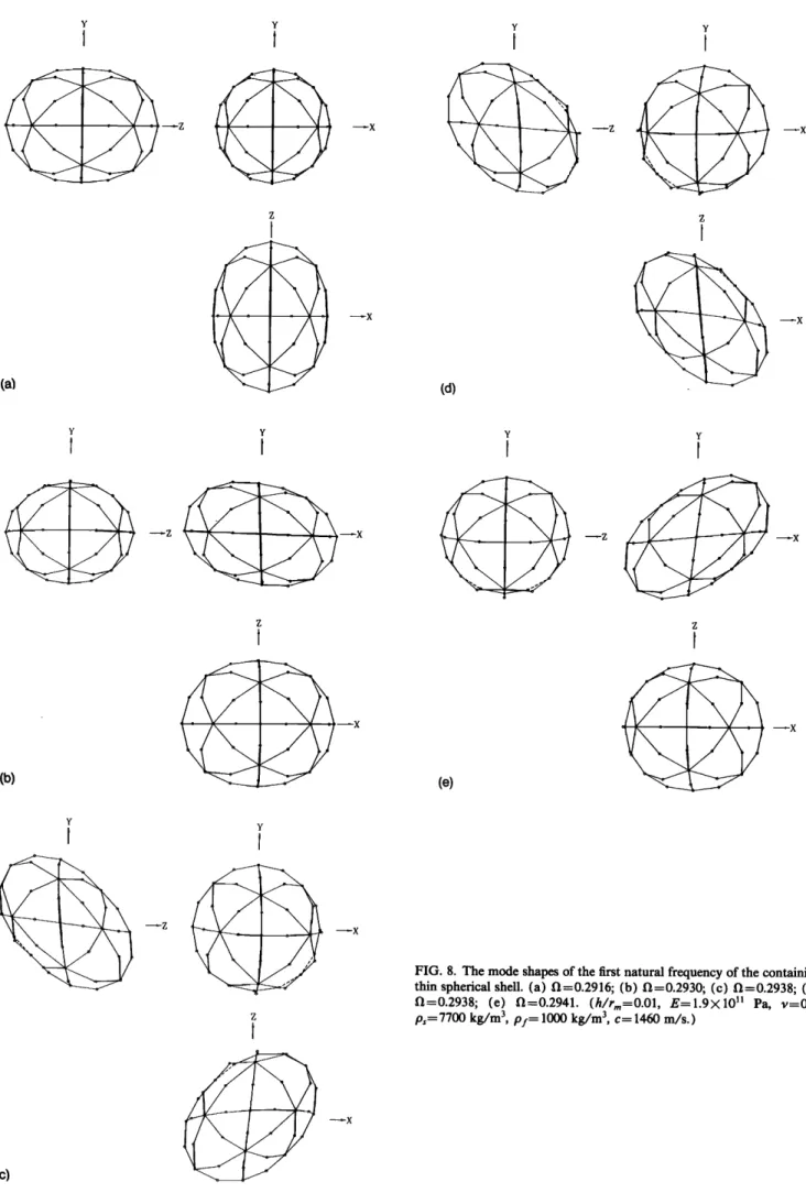
ample, the singular values in the neighborhood of the first natural frequency (approximately 0.29) of the containing shell with the thickness to radius ratio 0.01, calculated by using the mesh type A, are shown in Fig. 7. It can be seen from the number of singular value dips, the multiplicity of this natural frequency is 14- 1 4- 2 4- 1 = 5. The mode shapes of the same case are shown in Fig. 8. Comparison of the mode shapes in Fig. 5 with those in Fig. 8 shows great resemblance of the shell responses, with and without the fluid loading.

In addition to thickness to radius ratio, the effect of the material properties also plays an important role in the sound-structure interaction problems. In the following simulation cases, the thickness to radius ratio is maintained constant for comparing the interaction effects due to dif- ferent kinds of fluids. Consider a containing spherical shell having the following material properties: rm=l.0 m,

h/rm=O.01,

E=7.0X 10

•ø Pa, v=0.33, ps=2710.0

kg/m

3.

In order to evaluate interactions in a more quantitative

manner,

a coupling

index

2ø

G ( = pfc2S/(rn)

V, where

(rn)

is the average structural mass per unit area, S is the surface area, and V is the volume) is calculated for each case. Five kinds of fluids corresponding to five different orders of coupling (see Table III) are chosen for the simulation. Among these five cases, the first three cases are for air of low temperature and low pressure, high temperature and low pressure, and high temperature and high pressure sit- uations, respectively. The fluids of the last two cases are for pure water and mercury. The first two natural modes of the coupled systems are calculated for each case, by using the BEM-FEM algorithm. The analytical and numerical solu- tions of the natural frequencies of the shells with and with- out the fluid loading are compared in Table IV. As re- flected by the coupling index, it is found that the interaction between the shell and the fluid of very low density and sound speed is almost negligible. On the other hand, for air of high temperature and high pressure in case 3, significant changes of natural frequencies occur. This suggests that preventive measures must be taken against the damages caused by strong sound-structure interactions

I i i I I t I ! I I I. t t I 320 325 index number , 2 330 315 320 325 330 index number

(b)

index n•]mber index number

(c)

(d)

FIG. 7. Singular values of the containing thin spherical shell, corresponding to the first natural frequency. The y coordinate is plotted in the log scale.

(a) •=0.2916; (b) •=0.2930; (½) •=0.2938; (d) •=0.2941. (h/r,•=O.01, E= 1.9X l0 ll Pa, ¾=0.3, p,=7700 kg/m 3, pœ--1000 kg/m 3, c--1460

m/s.)

for thin-walled structures containing high temperature and high pressure gases, such as ramjet engines, pressure ves- sels, and nuclear reactors.

In summary, the structure and fluid can be approxi- mately treated as uncoupled systems for the situations of weak interactions. The natural frequencies of the fluid- loaded structure resemble the original structure in vacuo. On the other hand, the natural frequencies of the fluid- loaded structure are generally different from those of the original structure in vacuo for the situations of strong in- teractions. The shift of natural frequencies depends entirely on the degree of interactions, as reflected by the coupling

index.

V. CONCLUSIONS

A hybrid numerical technique based on BEM and FEM has been developed to extract the natural frequencies and mode shapes of coupled fluid-structure systems. While use of this technique is not limited to simple geometries,

the free vibrations of elastic thin spherical shells containing compressible fluids are investigated in a simulation because of the availability of analytical solutions. The physical in- sights derived from the simulation results can be summa-

rized as follows.

For situations of strong interactions (e.g., a thin spher- ical shell containing a liquid or a gas of high temperature and high pressure), the dynamic characteristics of the cou- pled fluid-structure system can be significantly different from the original subsystems because of the fluid loading, while for situations of weak interactions, the coupled sys- tem can approximately be regarded as uncoupled systems. From the comparison of the natural frequencies of the shell with and without the fluid loading, it can be observed that the more strongly the structure interacts with the fluid, the larger the shifts of natural frequencies. For instance, the thickness to radius ratio is an important parameter in con- sidering sound-structure interactions. Strong interactions may arise when a very thin shell is filled with a heavy fluid.

Y Y y y Z Z (d) Y y y y (b) z z (e) ---x Y Y ---z (c)

FIG. 8. The mode shapes of the first natural frequency of the containing thin spherical shell. (a) II--0.2916; (b) II--0.2930; (c) II--0.2938; (d) I1----0.2938; (e) I1----0.2941. (h/rm----O.01 , E--1.9><10 • Pa, ¾--0.3,

ps=7700 kg/m 3, pϥ 1000 kg/m 3, c---- 1460 m/s.)

TABLE III. Material properties and coupling indices

G=(pjc2/{m))S/V for cases 1-5. (h/rm=O.01, E=7.0X10 lø Pa,

v=0.33, ps--2710 kg/m3.) Case p f c G 1 1.21 346 5.4 X 10 3 2 1.21 520 1.2X 104 3 32.31 520 3.2 X 105 4 998 1480 8.1X 107 5 13 600 1450 1.1X 10 9

Unlike the natural frequencies, the mode shapes of the structure do not seem to be markedly changed inasmuch as

the sound-structure interaction is concerned. The mode

shapes of the fluid-loaded structure remain rather similar to those of the structure in vacuo with only slight differ- ences in the response amplitudes and torsional angles.

The method of SVD proves to be useful in searching for natural frequencies of the coupled system, although it appears somewhat computationally expensive. More effi- cient algorithms may be sought to deal with this nonstand- ard type of eigenvalue problems.

The numerical results illustrated in this paper are lim- ited to only a few of the lower-order natural frequencies, not only because the computation requires enormous CPU time, which is beyond the computer resources available, but also because the FEM codes for the thin spherical shell developed in this study do not seem robust enough for extracting higher-order modes. In any event, one ought to recognize the fact that these types of numerical methods

TABLE IV. Nondimensional natural frequencies f•=COrm/C p of the thin

containing spherical shell filled with different media. (h/rm=O.01,

E=7.0X 10 •ø Pa, v=0.33, ps=2710.0 kg/m3; case 1:pf=l.21 kg?m 3, c=346 m/s; case 2: p f--1.21 kg/m 3, c--520 m/s; case 3:pf=32.31 kg/m 3, c=520 m/s; case 4:pf=998 kg/m 3, c=1480 m/s; case 5: pf--13 600 kg/m 3, c-1450 m/s.)

Case

Mode Spherical shell Coupled system

order

n exact numerical exact numerical

1 2 0.689 0.687 0.694 0.696 1 3 0.818 0.863 0.820 0.867 2 2 0.689 0.687 0.682 0.696 2 3 0.818 0.863 0.809 0.847 3 2 0.689 0.687 0.639 0.646 3 3 0.818 0.863 0.759 0.782 4 2 0.689 0.687 0.181 0.186 4 3 0.818 0.863 0.239 0.258 5 2 0.689 0.687 0.0514 0.0529 5 3 0.818 0.863 0.0683 0.0753

are suited for only low-frequency analyses because of the limitation of resolution, e.g., the discretization spacing should not be greater than one half of the wavelength, as a rule of thumb. If high-frequency applications are of inter- est, one should resort to alternative approaches, such as the

statistical

energy

analysis

(SEA).21

Quantitative approaches for interpreting resonance phenomena of coupled sound-structure systems with ref- erence to the degree of interaction remain to be explored through numerical as well as experimental investigations in

the future.

ACKNOWLEDGMENT

The work was supported by the National Science Council in Taiwan, Republic of China, under the project

number NSC-80-040 l-E009-13.

•J. J. Faran, "Sound scattering by solid cylinders and spheres," J.

Acoust. Soc. Am. 23, 405-418 (1951).

2 M. C. Junger, "Sound scattering by thin elastic shells," J. Acoust. Soc.

Am. 24, 366-373 (1952).

3 L. H. Chen and D. G. Schweikert, "Sound radiation from an arbitrary body," J. Acoust. Soc. Am. 35, 1626-1633 (1963).

40. C. Zienkiewicz, D. W. Kelly, and P. Bettess, "The coupling of the

finite element method and boundary solution procedures," Int. J. Num. Eng. 11, 355-375 (1977).

5D. T. Wilton, "Acoustic radiation and scattering from elastic struc- tures," Int. J. Num. Meth. Eng. 13, 123-138 (1978).

6S. W. Wu, "A fast, robust, and accurate procedure for radiation and

scattering analyses of submerged elastic axisymmetric bodies," Ph.D. thesis, London University (1989).

7 A.D. Pierce, Acoustics (McGraw-Hill, New York, 1981).

8G. F. Roach, Green's Functions (Cambridge UP, New York, 1982). 9p. K. Banerjee and R. Butterfield, Boundary Element Methods in En-

gineering Science (McGraw-Hill, New York, 1981).

•øM. C. Junger and D. Feit, Sound, Structures, and Their Interaction

(MIT, Cambridge, MA, 1972).

•H. Kraus, Thin Elastic Shells (Wiley, New York, 1967).

•2A. H. Shah, C. V. Ramkrishnan, and S. K. Datta, "Three-dimensional and shell-theory analysis of elastic waves in a hollow sphere," J. Appl.

Mech. 36, 431 •.•.•. (1969).

•3R. D. Cook, D. S. Malkus, and M. E. Plesha, Concepts and Applications

of Finite Element Analysis (Wiley, New York, 1989).

•4j. W. Bull, Finite Element Applications to Thin-Walled Structures

(Elsevier Applied Science, New York, 1990).

•50. C. Zienkiewicz, R. I. Taylor, and J. M. Too, "Reduced integration

technique in general analysis of plates and shells," Int. J. Num. Meth. Eng. 3, 275-290 ( 1971 ).

•6W. Weaver, Jr., and P. R. Johnston, Finite Elements for Structural

Analysis (Prentice-Hall, Englewood Cliffs, NJ, 1984).

17I. C. Mathews, "Numerical techniques for three-dimensional steady-

state fluid-structure interaction," J. Acoust. Soc. Am. 79, 1317-1325 (1986).

•SB. Noble and W. Daniel, ,4pplied Linear/11gebra (Prentice-Hall, En-

glewood Cliffs, NJ, 1988).

•9j. S. Arora, Introduction to Optimum Design (McGraw-Hill, Singapore,

1989).

2øF. Fahy, Sound and Structural Vibration (Academic, London, 1985). 2• R. Lyon, Statistical Energy Analysis of Dynarnic Systems (MIT, Cam-

bridge, MA, 1975).