國
立
交
通
大
學
資訊科學與工程研究所
博 士 論
文
電腦視覺為基礎之多部位人體追蹤系統設計
Design of a Computer Vision-Based Multi-Part
Human Tracking System
研 究 生:趙善隆
指導教授:李錫堅 教授
電腦視覺為基礎之多部位人體追蹤系統設計
Design of a Computer Vision-Based Multi-Part
Human Tracking System
研究生: 趙善隆
Student: San-Lung Zhao
指導教授: 李錫堅
Advisor: Hsi-Jian Lee
國 立 交 通 大 學
資 訊 科 學 與 工 程 研 究 所
博 士 論 文
A Dissertation
Submitted to Department of Computer Science and Engineering College of Computer Science
National Chiao Tung University in partial Fulfillment of the Requirements
for the Degree of Doctor of Philosophy
in
Computer Science and Engineering June 2009
Hsinchu, Taiwan, Republic of China
i
電腦視覺為基礎之多部位人體追蹤系統設計
研究生: 趙善隆
指導教授: 李錫堅
國 立 交 通 大 學 資 訊 科 學 與 工 程 研 究 所
摘 要
本研究我們提出一個在錄影序列中之多部位的人體追蹤系統,首先我們利用一個背 景模型偵測並切割出錄影資料中之人體,由於背景影像通常成區塊變化,空間特性可用 來表示背景的外觀,為了要建立背景外觀的空間特性的模型,我們為成對的點上之組合 顏色建立混合高斯分布的模型。當人體被偵測及切割出來後,接著我們使用人體部位外 觀當作特徵並且使用粒子濾波器作為核心來追蹤此人體,我們採等化之顏色統計表當作 粒子濾波器中使用的外觀特徵以強化不同物體的鑑別率,為了建立可穩健區別目標物及 背景物體的追蹤器,我們同時使用目標的模型和背景模型來計算目標物的相似度,為了 對抗背景及目標物的外觀變化,背景模型及目標物模型都是可適應變化的。在一個粒子 濾波器中,當粒子數量很多時,特徵抽取的過程會有多餘的重複計算而沒有效率,為了 加速特徵抽取,我們為每張影像建立了數張累加的統計圖,每一個粒子的顏色統計表可 因此在常數時間中被計算出來。當追蹤人體的時候,我們會把人體切割為三個部位:頭、 軀幹、臀腳,這三個部位會分別被表示成為內縮的矩形並用粒子濾波器來追蹤,因為這 樣的處理,我們可以檢查這三個部位的一致性以減少可能的追蹤失敗,當追蹤過程中追 蹤狀態被更新後,我們會用支持向量機(SVM)來偵測追蹤錯誤並且判斷不正常的部位, 假如只有一個部位不正常,我們會校正這個不正常的部位並利用系統動態模型來追蹤此 部位,假如兩到三個部位不正常,我們就會從出此三個部位的預估位置重新初始化這三 個部位的追蹤。實驗結果顯示,我們提出的背景模型可以有效的偵測背景有改變時及物 體在原地移動時的移動物體區域,跟高斯背景模型和混合高斯背景模型比較,我們提出ii 的方法可以抽取出更完整的移動物體區域。人體追蹤的實驗顯示出,我們提出的三部位 人體追蹤及錯誤校正可以正確持續追蹤 95%的人高達 105 個畫面,考慮人體部位追蹤, 我們提出的系統可以持續追蹤頭部、軀幹、臀腳這三個部位 105 個畫面的正確率分別高 達 95%、83%、91%,和整個人體視為一個部位的追蹤作比較,正確率提升 20%,這個結 果顯示出這個系統是一個有效的追蹤系統。
iii
Abstract
The study presents a multi-part human tracking system in video sequences. First, we detect and extract humans in a video according to a background model. Since background images usually change in blobs, spatial relations are used to represent background appearances. To model the spatial relations of background appearances, the joint colors of each pixel-pair are modeled as a mixture of Gaussian (MoG) distributions. After the human is detected and extracted, we then track body parts of the human by using appearances of these parts as the features and using particle filters as the tracking kernel. In the particle filter, we adopt color histograms as the appearance features and use a specific histogram mapping to enhance the discriminability between different objects. To form a robust tracker that can distinguish target objects from background objects that have color distribution similar to those of target objects, we calculate the target similarity from both the target object model and the background model. To handle the appearance variations of background and target objects, both the models of the background scene and the target object are adaptable. In a particle filter, when the number of particles is large, the feature extraction is repeated redundantly and inefficiently. To speed up feature extraction, we create a cumulative histogram map from each image. The color histograms of each particle can then be extracted in constant time. When tracking a human, we decompose the human body into three parts: head, torso, and hip-leg, represent them by three shrunk rectangles, and track them by particle filters. In this way we can reduce possible tracking failures by checking the consistency of states among these three parts. After the tracking states are updated, we use support vector machines (SVM) to detect tracking failures and abnormal body parts. If a single part is abnormal, we adjust its position and use the system dynamic model to track the abnormal one. If two or three parts are abnormal, we re-initialize the tracking process of the three parts around their predicted
iv
positions. Experimental results show that the proposed background model can be used to efficiently detect the moving object regions when the background scene changes or the object moves around a region. By comparing with the Gaussian background model and the MoG-based model, the proposed method can extract object regions more completely. The experimental results of human tracking showed that the proposed three-part tracking system with failure detection and correction can track correctly about 95% persons until the 105th frame. With respect to the body parts, our system has about 95%, 83%, and 91% tracking rates for the head, torso, and hip-leg parts respectively until the 105th frame. The tracking rate of a human increases 20% comparing with that of the whole-body tracker. These rates show the effectiveness of the proposed system.
v
誌謝
本論文的完成,首先必須感謝我的指導教授李錫堅老師,由於他長期以來的教誨及 指導,才能完成我的研究。其次我要感謝的是所有口試委員:陳稔教授、蔡文祥教授、 范國清教授、廖弘源教授、黃仲陵教授及余孝先老師,由於諸位老師給予的寶貴建議與 指正,使的本論文的內容更加完整。 感謝對我的研究方向及研究態度有著重要啟發的實驗室學長們:曾逸鴻教授、蔡俊 明教授、盧文祥教授、陳俊霖博士、楊希明學長、鄭紹余學長。另外還要感謝在實驗室 跟我共同研究的同學及學弟們:王舜正、游以正、陳映舟、黃仁贊、吳杭芫、呂偉成、 張倍魁、林欣頡、林俊隆、劉一葦、陳思源、曹育誠、陳威甫、陳大任、郭文傑、林鍵 彰,在研究的內容及日常生活上,實驗室同伴們都對我有著莫大的幫助,由於大家長期 的陪伴,讓我能夠繼續我的研究。 感謝在我到花蓮時提供我許多協助的朋友及學弟妹們,尤其要感謝許展榮先生在我 剛到花蓮時,熱心陪我找住所及帶我了解花蓮的環境,感謝邱奕廉和林柔依對我多次到 花蓮時交通和居住上的幫助,感謝歐陽儒及陳文祥對我花蓮生活上的幫助,在花蓮幫助 過我的朋友太多了,難以一一列舉,由於花蓮朋友們的幫助,我才能順利度過研究的最 後難關,因此由衷感謝這些朋友們。 當然還要特別感謝一路支持我的家人們,由於父母親及岳父岳母一直以來給我的支 持,讓我更堅定要完成研究的信念。當然更要感謝我的妻子菱芝一直以來對我的包容與 鼓勵,在我許多次要放棄研究時,都是因為妻子的鼓勵我才能繼續堅持下去。 最後誠摯的以此研究成果獻給所有幫助過我的人們。 趙善隆 九十八年鳳凰花開時於新竹vi
目錄
摘 要 ... i Abstract ... iii 誌謝 ... v 目錄 ... viList of Figures ... ix
List of Tables ... xi
1. Introduction ... 1
1.1 Background Subtraction ... 1
1.2 Human Tracking ... 3
1.3 Organization of This Dissertation ... 7
2. Related Works ... 8
2.1 Background Subtraction ... 8
2.2 Human Tracking ... 13
3. A Spatially-Extended Background Model ... 19
3.1 Joint Background Model ... 19
3.1.1 Spatial Relation in Images ... 19
3.1.2 Calculation of Background Probabilities ... 20
3.1.3 Estimation of Bivariate Color Distributions ... 22
3.2 Saptially-Dependent Pixel-Pairs Selection ... 26
4. A Particle Filter with Discriminability Improved Histogram Model ... 27
vii
4.1.1 Prediction ... 27
4.1.2 Particle Weighting ... 29
4.1.3 Particle Selection ... 30
4.2 Target Object Similarity ... 31
4.2.1 Specific Histogram Mapping ... 32
4.2.2 Target Appearance Model ... 33
4.2.3 Background Appearance Model ... 34
4.2.4 Similarity Measurement ... 34
4.3 Cumulative Histogram Map ... 36
4.4 Dynamic Number of Particles Adjustment ... 38
5. Three-Part Human Tracking and Consistency Checking ... 40
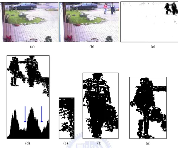
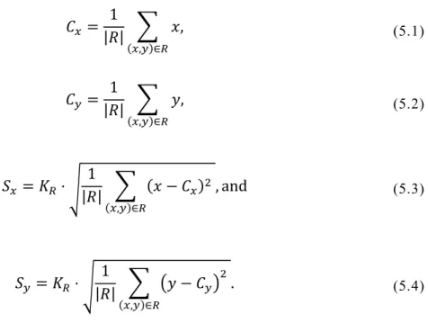
5.1 Human Extraction ... 40
5.2 Human Part Decomposition ... 42
5.3 Tracking Failure Detection ... 44
5.4 Tracking Failure Adjustment ... 46
5.4.1 Failure from Inter-Person Occlusion ... 47
5.4.2 Failure from Background Object Occlusion ... 48
6. Experimental Results ... 50
6.1 A Spatially-Extended Background Model ... 50
6.2 Adaptive Color-Based Particle Filter ... 59
6.2.1 The TCU Video Set ... 62
6.2.2 The CAVIAR Video Set ... 64
6.2.3 Specific Histogram Mapping ... 65
6.3 Tracking Failure Adjustment ... 68
viii
6.3.2 Analysis of Tracking Accuracy ... 69
6.3.3 Multi-person tracking ... 73
6.3.4 Tracking failure analysis ... 74
7. Conclusions and Future Works ... 75
ix
List of Figures
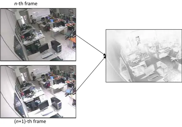
Fig. 1.1 Left column: two consecutive images in different illumination conditions. Right
image: intensity differences between the left two images. ... 2
Fig. 1.2 Example of the three body parts used on tracking a person. ... 4
Fig. 1.3 The system flow diagram of the three-part human tracker. ... 6
Fig. 2.1 An example of a slowly moving person. ... 10
Fig. 2.2 Sketches of a person whose clothes colors are similar to the door color in front of different background scenes. ... 11
Fig. 3.1 Color samples of three pixels in 1000 frames. ... 22
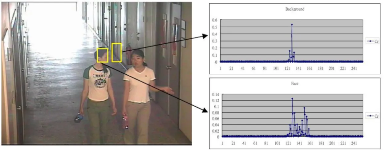
Fig. 4.1 A sample image and the histogram of the Cr channel in the two rectangles. ... 31
Fig. 4.2 The two histograms of the Cr channel in Fig. 4.1 quantized into eight bins. ... 31
Fig. 4.3 An example of the similarity measurement by using the color histograms of target person and background image. ... 35
Fig. 5.1 Foreground subtraction images. ... 41
Fig. 5.2 An example of human parts decomposition of a person. ... 43
Fig. 5.3 Examples of two types of tracking failure. ... 47
Fig. 6.1 Foreground detection results of an image captured by Cam1. ... 51
Fig. 6.2 Foreground detection results of an image captured by Cam2. ... 52
Fig. 6.3 Foreground detection results of an image captured by Cam3. ... 53
Fig. 6.4 Foreground detection results of the images captured by the three cameras. ... 55
Fig. 6.5 Test samples and the manually labeled ground truth masks used for estimating the ROC curves. ... 56
Fig. 6.6 The ROC curve of test images captured by Cam1. ... 57
x
Fig. 6.8 The ROC curve of test images captured by Cam3. ... 58
Fig. 6.9 Sample images of the four scenes in the TCU video set. ... 60
Fig. 6.10 Sample images and the tracking results of a target person. ... 61
Fig. 6.11 The trajectories of a target person. ... 62
Fig. 6.12 he tracked body parts using different color histogram models. ... 66
Fig. 6.13 The tracking results captured in an open space in front of a house. ... 67
Fig. 6.14 The tracking results in a corridor. ... 69
Fig. 6.15 Tracking rates without and with failure detection. ... 70
Fig. 6.16 The tracking results with failure adjustment and inter-person occlusion detection. . 71
xi
List of Tables
Table 1 Average Center Deviation by Different Similarity Measuement ... 63 Table 2 Tracking Speed by Different Similarity Measuement (fps) ... 63 Table 3 Average Center Deviation on The Caviar Video Set by Different Similarity
Measuement ... 64 Table 4 Tracking Speed on The Caviar Video Set by Different Similarity Measuement (fps) 64
1
1. Introduction
Human tracking is a fundamental and important step for many visual surveillance applications, such as security guard, patient care, and human-computer interaction. A human tracking system can be divided into two modules, human segmentation and human tracking. The human segmentation module detects and segments a person in a frame. After the person is detected and segmented, the human tracking module then locates the positions of the person in the following frames.
1.1 Background Subtraction
In an indoor environment, people are usually considered to be the only foreground objects, which are defined as ego-motion objects. If the images with only background objects can be captured in advance, the positions of a human can be detected by comparing the current image with the background images. However, background images vary when camera positions, background object positions, and illuminations change. Tracking objects in general environments will become very complicated.
In many surveillance applications especially in indoor environments, camera positions are generally fixed. Illumination variations and background object motion may change the captured images significantly. Examples of the motions include placing a book on a desk and moving a chair to another position. The positions of the objects are usually changed by people or other external forces. After the motion stops, these objects remain in the same position for a certain period; these motions are usually not repeated. In an indoor environment, the illumination of objects is not affected by continuous light changes, such as sun rise, sun set, or weather changes. Ignoring these continuous changes, brightness variations such as turning lights on or off, as shown in Fig. 1.1, and opening a window are assumed to be abrupt. Several
2
researchers [1] assumed that brightness variations due to illumination changes are uniform. The right-hand side image in Fig. 1.1 shows the intensity differences after the lights were turned on. We observe that brightness variations in different pixels are not uniform. It is difficult to process this kind of variations. Several other researchers [1-4] assumed that illumination changes are not repeated like the motion of freely movable objects. However, light sources can be repeatedly turned on or off several times over a period of time. The appearance changes on the illuminated regions will also be repeated.
To model the non-repeated background changes, we can use an online updating scheme to adapt to the background appearances in recently captured images [1-17]. When the appearances of a pixel repeatedly change, they can be modeled as a Mixture of Guassians (MoG) [9]. The online updating MoG model is useful for modeling rapidly repeated
n‐th frame
(n+1)‐th frame
Fig. 1.1 Left column: two consecutive images in different illumination conditions. Right image: intensity differences between the left two images.
3
background appearances such as waves on water surface, but does not works well in long-term repeated appearances such as door opening and closing. In consecutive images, the repeated appearances of background objects usually appear in blobs in fixed places, while the appearances of foreground objects usually change their places and do not form fixed blobs. In this study, we extend the MoG model by using the spatial relations among pixels to model the background appearances.
The objective of our system is to extract moving object from a sequence of images. The system is divided into two modules: background modeling and foreground detection. The first module creates a background model to represent possible background appearances. The parameters of the model are learned and updated automatically from recently captured images. In the background model, the distributions of background features are assumed to be mixtures of Gaussians [9]. Since background appearances are changed in blobs, the features used in the MoG should be able to represent spatial relations in the blobs. To represent the spatial relations, we estimate the joint color distributions of pixel-pairs in a short distance. Since estimating the distributions of all pixel-pairs is costly and not all pixel-pairs provide enough information to model background, we first calculate the dependence of colors in each pixel-pair. A pixel-pair with a higher color dependency implies that the two pixels provide more information to represent the appearance changes in blobs. Highly dependent pixel-pairs are then selected to model the spatial relation of background. In the second module, the background model that has already been updated from recent images is used to calculate the background probability of each pixel of the current image. The probability is then used to decide whether the pixel belongs to the foreground or background. Connected foreground pixels are extracted to form foreground regions.
4
To track an object in a sequence of frames, we can model appearances of the object and then use the model to predict its position in the sequence. However, in a complex environment, detecting a target object using the appearance model in video sequences is not easy since the appearances of the object are variable due to occlusion, illumination variations, or orientation changes. In general, the movements of an object in consecutive frames are assumed smooth. Therefore, if we can locate the target object in several frames, the appearance model and movement model of the target object obtained from these frames can be used to track the object in the following frames.
In this study, we aim to create the trajectory of a human and predict his positions for safeguarding, that is, to detect an intruder approaching a building or a designated place. Since a human is not a rigid object, his appearance might be greatly affected by his motion. We decomposed the human body into three parts: head, torso, and hip-leg, since the three parts usually have different appearances and can be distinguished as shown in Fig. 1.2. The images show that the colors of the head part contain mostly skin colors and hair colors, which are
Fig. 1.2 Example of the three body parts used on tracking a person. The three body parts are shrunk and the limbs are excluded to reduce the affection from human motion.
5
usually different from the colors of the other two parts. The colors of the torso and hip-leg parts consist mainly of those of the clothes, which may be similar, as shown in the fourth and fifth images of Fig. 1.2. To separate the three parts, we have to use other features such as height ratios.
With respect to the features used, we adopted color histograms proposed by Perez et al. [18] and Nummiaro et al. [19] to model the appearances of the three body parts. In the initialization phase, we adopted the background subtraction method according to a Gaussian background model to extract a human and then extract the histograms of the body parts from the human region. We then tracked the humans by using their appearances as the features and tracked the three parts by particle filters to reduce possible failures due to appearance changes by checking the consistency of states among these three parts. Since the appearance model of each person in recent frames was usually unique and temporally context-dependent, the model can be used to distinguish different persons and track them independently. However, when modeling the color histogram in the whole color space, histogram matching was time-consuming due to the high dimensional features used. The method proposed by Nummiaro et al. [19] quantized the color histogram into an 8 8 8 or 8 8 4 three-dimensional one. The method proposed by Perez et al. [18] modeled colors in HSV color space by two histograms. The intensity channel was modeled as a histogram and the other two channels as another two-dimensional histogram. The histograms were quantized into several bins to improve the speed and reduce the effect of noise. However, in these models, two objects with very few dissimilarities were not easily distinguished. In our research, we propose a specific histogram mapping for histogram feature extraction to improve the ability of discriminating the objects with similar color distributions. Since the camera in our system is fixed, the background scene can be assumed less changed in consecutive frames. To improve the discriminability between the target object and background
6
objects, we combined the adaptive background model with the adaptive color histogram model of the target object.
When adopting the color histograms as the features used in a particle filter, we need to extract the histogram feature for each particle. It is generally very inefficient to extract the features for a large number of particles. In this research, we will create a cumulative histogram map (CHM) for each image to improve the efficiency of feature extraction. The cumulative histogram map is similar to the integral map that is popularly used for extracting Haar-Like features [20]. They will be modified to cumulate the histogram features of each sample state in constant time.
For failure detection and adjustment, we will use a support vector machine (SVM) [21,22] to distinguish abnormally and normally tracked body parts. The position of an abnormal body part will be adjusted according to its relative positions with the other body parts. If a single part was abnormal, we adjusted its position and used the system dynamic model to track the abnormal one. If two or three parts were abnormal, we re-initialized the tracking process of the three parts around their predicted positions. Next, we detect whether the failure is caused by occlusion or similar appearances. For the latter case, we will estimate
7
the appearance model from the adjusted rectangle of the body parts; else, the appearance model is kept unmodified. The flow diagram of our tracking system is depicted in Fig. 1.3. It includes four major modules: initialization, particle-filter-based tracking, abnormal body part detection, and state correction.
1.3 Organization of This Dissertation
The rest of this dissertation is organized as follows. Chapter 2 is a review of related research. Chapter 3 describes the proposed spatially-extended background model. Chapter 4 describes the particle weight measurement and the cumulative histogram map used to improve the calculation speed. Chapter 5 describes the three-part human tracking and consistency checking for failure adjustment. Chapter 6 gives experimental results and their analysis. Finally, Chapter 7 presents the conclusions and future works.
8
2. Related Works
2.1 Background Subtraction
A background model in a surveillance system represents background objects. The method that compares the current processed image with the background representation to determine foreground regions is called background subtraction. If the background is unchanged but affected by Gaussian noise, the colors of the background pixels can be modeled as a Gaussian distribution with mean vector (µ) and covariance matrix (Σ) [1-8]. Background subtraction is then performed by calculating the probability of each pixel in the current image belonging to the Gaussian model.
Since background appearances may be affected by external forces, modeling a pixel with a Gaussian distribution may misclassify some background pixels as foreground ones. In many cases, the background may change repeatedly. A background pixel with repeated changes can be divided into several background constituents and modeled as an MoG distribution [9-13]. For each background constituent in a pixel, the means ( ), covariances (Σ ), and weights ( ) of the i-th constituent ( ) have to be estimated. If there are K background constituents, the parameters of the background model can be represented as , Σ , |1 In order to decide whether a sample point X belongs to the background B, the conditional probability | is calculated as follows:
9
where η represents a Gaussian probability density function, ; , Σ 1
2 / |Σ | / . (2.2)
The motion of some background objects may not be repeated. After the motion, the objects remain in the same position for a period. To model the background changes, researchers have proposed methods for online updating of the parameters of background models [1-17]. The mean vector and covariance matrix in time t are represented as and Σ , respectively. The updating rules are formulated as follows:
1 , (2.3)
Σ 1 Σ , (2.4)
where ρ is used to control the updating rate. To integrate the updating method into an MoG model, Stauffer and Grimson [9] proposed a method to update the mean vector and covariance matrix of a background constituent to match those of in Eqs.(2.3) and (2.4). The weight , of the i-th background constituent is updated as follows:
, 1 , , , (2.5)
where , is an indicator function, whose value is one if the i-th background
constituent matches and zero otherwise, and α is a constant used to control the updating rate of the weights. In Stauffer and Grimson's method [9], the updating rate ρ for the parameters of the i-th constituent (Gaussian distribution) is calculated according to α and ; , Σ .
To make background models more robust, researchers tried to modify updating rules or adopt different features [10-13]. In adaptive background models, background objects are assumed to appear more frequently than foreground ones. However, the
10
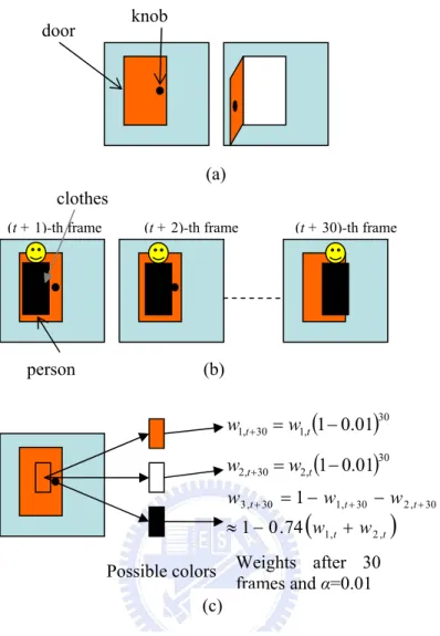
assumption is not always satisfied. If the appearances of a background pixel appear less frequently than those of foreground objects, the background pixel is probably misclassified as a foreground object. Taking the following case as an example, assume a room is monitored by a fixed camera and the background objects in the room include a door and a wall as shown in Fig. 2.1(a). People may enter the room, and close or open the door. If a person wears a suit of clothes of single color and walks
person
(a)
(b)
(t + 1)-th frame (t + 2)-th frame (t + 30)-th frame
Possible colors Weights after 30 frames and α=0.01
(
)
30 , 1 30 , 1t+ =w t 1−0.01 w(
)
30 , 2 30 , 2t+ =w t1−0.01 w(
t t)
t t t w w w w w , 2 , 1 30 , 2 30 , 1 30 , 3 74 . 0 1 1 + − ≈ − − = + + + door knob clothes (c)Fig. 2.1 An example of a slowly moving person. (a) Sketches of two possible background scenes. Left: door closed; Right: door opened. (b) Consecutive frames of a person moving from left to right. (c) Possible colors and their weights of the rectangle region shown in the left image.
11
slowly across the room as shown in Fig. 2.1(b), the major color of the clothes may be captured repeatedly in a certain position among several consecutive images. Assume that the person moves from left to right in 30 frames. If the updating rate α in Eq.(2.5) is set as 0.01, the weight of the repeatedly captured color of the clothes in the images will increase from 0 to 0.26, as shown in Fig. 2.1(c). This large weight may cause the clothes to be labeled as the background, when the MoG model in Eq.(6.2) is used. Using a small updating rate can overcome this problem; however, the background model will be updated very slowly and may fail to learn background changes.
In another situation, the color of the person's clothes is assumed to be the same as that of the door, as illustrated in Fig. 2.2(a). If the person enters the room and passes through the door, the region of clothes may be labeled as background due to the similarity of colors. However, after the door is opened, the current background color is not similar to the clothes color as shown in Fig. 2.2(b). The clothes may still be labeled as the background, since they are very similar to possible background colors been estimated.
In these two situations, we observe that modeling each pixel independently
(a) (b)
Fig. 2.2 Sketches of a person whose clothes colors are similar to the door color in front of different background scenes: (a) scene when the door is closed and (b) scene when the door is opened.
12
cannot sufficiently represent the similarity among different object appearances caused by either object motion or illumination changes. Most researchers regarded the variations caused by object motion as foreground changes and attempted to eliminate the effect caused by illumination. In consecutive images, when the illumination changes, the pixels of an object are usually changed simultaneously. In order to model background objects, the pixels at different positions should be considered together. To represent the relation among the pixels, Durucan and Ebrahimi [14] proposed to model the colors of a region as vectors. They segmented the foreground regions by calculating the linear dependence between the vectors of the current image and those of the background model. However, it is expensive to represent the dependence between vectors in terms of storage and speed. To reduce the cost, the vector of a region should be reduced to a lower dimensional feature. Li et al. [15,16] used two-dimensional gradient vectors as the features of local spatial relations among neighboring pixels. In their proposed method, the appearance variations caused by illumination changes can be distinguished from object motion. However, the gradient features cannot be used to extract the foreground region that has a uniform color. To model the relation among pixels, we need to use the relations among near pixels to reduce time and storage consumption, and then extend the relations into a more global form.
The methods based on the Markov random field (MRF) are well known for extending the neighboring relations among pixels into a more global form. Image segmentation methods based on MRF [17,23] assume that most pixels belonging to the same object have the same label and these pixels form a group in an image. The MRF combines colors among a clique of pixels in a neighboring system and uses an energy function to measure the color consistency. Then, the maximum a posterior
13
estimation method is used to minimize the energy for all the cliques to find the optimal labels. In the MRF-based methods, the final segmentation results are strongly dependent on the energy functions of the labels in different cliques. If a high energy is assigned to the clique with unique labels, the extracted foreground regions will become more complete than those of the pixel-wise background models. An additional noise removal process is not required. However, when several pixels are mis-labeled, these errors will propagate into neighboring pixels. The error propagation will cause more pixels to be mis-labeled. In this research, we directly estimate the relations among pixels instead of the labels, and therefore the errors will not easily propagate.
2.2 Human Tracking
In the last few decades, tracking objects or humans in video sequences has received much attention. Much research about the topic has been proposed and been reviewed in several survey papers [24-28]. Moeslund et al. [24] divided a general human tracking algorithm into two main phases: figure-ground segmentation and
temporal correspondences. The former finds the target human in an image, and the
latter associates the detected humans in consecutive frames to create temporal trajectories. In the following, related work about these two phases will first be addressed. The methods for segmenting human bodies and correcting tracking failures will then be described.
The methods of figure-ground segmentation can be classified into five categories according to the used features. These categories include background subtraction [6,9],
motion-based segmentation [29], depth-based segmentation [30], appearance-based segmentation [18,19,21,31,32], and shape-based segmentation [2,33]. Background
14
subtraction and motion-based segmentation methods find the differences between images to extract the target. The two approaches assume that only one target object moves in a specific region and the appearances of background objects in consecutive images do not change. However, the assumptions usually cannot be met in general environments. To achieve better segmentation results for tracking, further checks are needed. The depth-based segmentation approach uses the positions of the target in three-dimensional space or in the ground plane to segment the target. However, to locate such kind of positions, specific hardware (such as multiple cameras) or additional calculations (such as inverse perspective transform) are needed. The appearance-based segmentation approach became popular recently, since the approach is usually simple and fast. The approaches of shape-based and appearance-based segmentation are similar except that the former does not use the color content inside the object. Since the appearances of a tracking target may change with time, several researchers proposed methods to model and update the appearance model of the target person dynamically in consecutive images [19,32]. Since the target is a moving object, some researchers tried to segment the target by a background subtraction method [6,9,34]. Shan et al. [34] modeled the colors of the target object as the appearance feature and then use the color cue to calculate a color probability distribution map from the current image. The color probability distribution map was combined with the background subtracted image using a logical AND operation to detect the target position. Other researchers used classifiers such as SVM [21] and Adaboost [31] to model the appearance of target objects.
In the tracking phase, temporal correspondence aims to predict and update the states of the target person from the measurement and predicted state, where the measurement is detected by figure-ground segmentation and the predicted state is
15
calculated using the system dynamic model. To find the temporal correspondences, Polat et al. [35] used MHT (Multiple Hypothesis Tracker) to construct hypotheses representing all the predictions and measurements. The most likely hypothesis is chosen as the target. To combine the predictions and measurements, Kalman filtering is another well-known method and has already been applied in many studies [3,9,36]. The Kalman-filter-based approaches are commonly used for tracking a target whose system dynamic model can be represented as a linear function and the noise as a Gaussian. In non-linear systems, extended Kalman filters that approximate the non-linear dynamic model by Taylor series have been applied [37]. Recently, particle filters have been proposed to construct a robust tracking framework that are neither limited to linear dynamic model nor Gaussian distributed noise [19,38,39]. The method represents the state of a target object by a set of samples (particles) with weights. The weight of a sample is calculated by the figure-ground segmentation and the samples are generated by the importance sampling method so that the samples can represent the probability distributions of the target object's appearances. We adopt the particle filter in our system, since they can be applied in an appearance-based tracking system very effectively.
A human is not a rigid object and his appearance changes irregularly. Segmentation of human body parts in an image has already been proposed in several papers [40-43]. Forsyth and Fleck [40] introduced the notion of 'body plans' to represent a human or an animal as a structured assembly of body parts learnt from images. Shashua et al. [41] divided a human body into nine regions, for each of which a classifier was learnt based on features of orientation histograms. Mikolajczyk et al. [42] divided a human body into seven parts. For each part, a detector was learnt by following the Viola-Jones approach applied to scale invariant orientation-based
16
features. Ioffe and Forsyth [43] decomposed the human body into nine distinctive segments. The method finds a person by constructing assemblies of body segments. The segments were consistent with the constraints on the appearance of a person that result from kinematic properties. These body-parts-based human segmentation methods usually focused on detecting humans in a static image. Recently, body-parts-based human tracking in consecutive images has been proposed [21,31,44-47]. Parts of these studies focused on precise decomposition of body parts for motion type or pose analysis. However, in general environments, it is difficult to decompose precisely body parts due to self occlusions and complex background scenes. The studies in [21,47] proposed a detection-based tracking model to solve the occlusion problem. They detected body parts by a pretrained model, and then tried to associate the detected body parts to a target person by smoothing his trajectory. However, when multiple humans appeared in a frame, the detection model could not differentiate the body parts of the different persons. The spatial positions and velocities were the only cues, which can be used to find the temporal correspondences of different persons.
When a person is tracked in consecutive frames, the figure-ground segmentation may fail, since the person may be occluded or other objects may have similar appearances with the target person. The first problem can be classified into occluded by other persons and occluded by background objects. To cope with the problem of inter-person occlusion, several researchers proposed to detect occlusion events and then used the system dynamics to estimate the position of the occluded person [48,49]. Using similar methods to predict the occlusion of background objects, one needs to create background object models. However, it is difficult to model all background objects in a complex environment. Several researchers tried to cope with the
17
occlusion problems by tracking different body parts of a person simultaneously [21,47,48]. When a body part is occluded, the position of the person can still be tracked based on the other parts. Mohan et al. [21] extracted a human body by detecting four parts: the head, legs, left arm, and right arm, by four distinct quadratic support vector machines. After geometric constraints among these parts are confirmed, another support vector machine is used to classify the combination of the four parts as either a human or a non-human. Wu and Nevatia [47] used four detectors to detect head-shoulder, torso, legs, and full-body. The detectors were learnt by a boosting approach using edgelet features. They used a strong classifier to classify the body parts in images. When we track multiple humans, the classifier cannot be used to distinguish different persons, and their trajectories will easily be confused if no other approaches are adopted. Lerdsudwichai et al. [48] proposed a method to model the face and clothes in the initialization phase. To identify different persons, they used clothes colors. However, the appearance of a person may change when the person presents different poses or is affected by different illuminations. The appearances captured in the initialization phase cannot be applied to track the person in other frames. In our research, we use an adaptive appearance model to track the body parts, even when multiple persons are tracked.
Apart from the occlusion events, a tracker may lose the tracking target when other objects have similar appearances. In general, a robust appearance model can be used to reduce the tracking failures, or the system dynamic model of the target person can be used to predict his position. However, the robust appearance model may be too complex to maintain efficiently. We will use the system dynamic model of the target person to track him, when a tracking failure is detected. To detect the tracking failure, Dockstader and Imennov [36] proposed a method that uses a structural model to
18
represent a person and a hidden Markov model (HMM) to describe the temporal characteristics of the tracking failure. In the tracking phase, the HMM was used to predict the tracking failures. Since a person may change his velocity, the predicted position of the person using the system dynamic model is too rough. A fine tune for the target person is needed.
19
3. A Spatially‐Extended Background Model
In the initialization step of a tracking system, the human region in a image needs to be segmented for tracking. To segment the human region, we create a background model and update it using recent background variations. Since background images are usually changed in blobs, spatial relations are used to represent background appearances, which may be affected drastically by illumination changes and background object motion. To model the spatial relations, the joint colors of each pixel-pair are modeled as a mixture of Gaussian (MoG) distributions. Since modeling the colors of all pixel-pairs is expensive, the colors of pixel-pairs in a short distance are modeled. The pixel-pairs with higher mutual information are selected to represent the spatial relations in the background model. Experimental results show that the proposed method can efficiently detect the moving object regions when the background scene changes or the object moves around a region. By comparing with Gaussian background model and the MoG-based model, the proposed method can extract object regions more completely.
3.1 Joint Background Model
In a sequence of images, colors will change in blobs instead of individual pixels due to illumination changes or object motion. This paper proposes to utilize the relations among pixels to represent the changes in blobs. The relations are formulated as a spatially-extended background model, which is then used to classify the pixels into either foreground or background.
20
Using pixel-wise features, if the color of a foreground pixel is similar to those of the background, the pixel may be misclassified as background. If we can estimate the distributions of color combinations for the pixels in blobs, the foreground objects can be classified more precisely. Suppose there is a red door in a room and the appearance outside the door is white. When a person wearing a suit of interlaced red and white stripes passes through the door, parts of the suit may be misclassified as background when the colors of the pixels are modeled independently. Nevertheless, if we model the background appearances among pixels using joint multi-variate color distributions, the interlaced red and white stripes can be classified as foreground using the method introduced later. However, estimating the multi-variate distributions for all pixel-pairs is still costly since the number of pixel combinations may be very large. In this research, we will estimate the color distributions of joint random vectors in closed pixel-pairs.
As stated in Sec. 2.1, illumination changes and background object motions may change background appearances. Since the changes are complex, it is difficult to collect enough training samples for all the possible changes. In this paper, we modify Eqs. (2.3) and (2.4) for updating the color distributions of pixel-pairs to adapt to the appearances that have not been trained, to be described in Sec. 3.1.3.
3.1.2 Calculation of Background Probabilities
Assume that we have already estimated the color distributions of all background pixel-pairs. In this research, we decide whether pixel belongs to foreground according to its color and the color combinations of pixel-pairs , , where A denotes a set of pixels associated with .
Suppose that a sequence of pixels , , … , has a corresponding color sequence , , … , . The probability of pixel belonging to background can be
21
represented as | , , … , , where the sequence , , … , denotes the joint random variable of the colors for the sequence , , … , , and represents the event that pixel a0 belongs to the background.
Assuming that , , … , are conditionally independent, based on the naive Bayes' rule, the probability | , , … , can be computed as the product of n pair-wise probabilities:
| , , … ,
| , .
(3.1)
When estimating the background probabilities from above equation, we face two problems. The first one is the estimation and updating of the probability distributions | , , , and . The distribution | , a pixel-wise background color distribution, is regarded as an MoG and can be calculated from Eq.(6.2), whose parameters are estimated and updated by using Eqs. (2.3), (2.4) and(2.5). It is tedious to estimate and update the bivariate probability distribution , , since the number of possible color combinations in and is large. We will simplify the estimation and updating by combining the MoGs of pixels to form the joint random vector distributions of pixel-pairs. The second problem is the cost of modeling pixel-pairs. To model all pixel-pairs, the number of pixel-pairs is , where W and H are the width and height of the images, respectively. We reduce the complexity by only modeling the pixel-pairs that can provide sufficient information to represent spatial relations as described in Sec. 3.2.
22
3.1.3 Estimation of Bivariate Color Distributions
As mentioned before, the color distributions of pixel-pairs should be updated to adapt to the background changes. If we assume the color distributions in a pixel-pair
0 50 100 150 200 250 x40.80 0 50 100 150 200 250 x3 0. 70 r(x1) r(x3) r(x2) 0 50 100 150 200 250 x30. 70 0. 00 0 0. 00 5 0. 01 0 0. 01 5 0 50 100 150 200 250 x40.80 0 50 100 150 200 250 x5 0. 90 (b) 0 50 100 150 200 250 x5 0. 90 0. 000 0. 005 0. 010 0. 015 0 5 0 1 0 0 1 5 0 2 0 0 2 5 0 x 4 0 . 8 0 0 . 0 0 0 0 . 0 0 5 0 . 0 1 0 0 . 0 1 5 0 . 0 2 0 R1 R2 R3 R4 (a) a1 0 50 100 150 200 250 300 1 72 143 214 285 356 427 498 569 640 711 782 853 924 995 R G B 0 50 100 150 200 250 300 1 72 143 214 285 356 427 498 569 640 711 782 853 924 995 R G B 0 50 100 150 200 250 300 1 73 145 217 289 361 433 505 577 649 721 793 865 937 R G B a2 a3
Fig. 3.1 Color samples of three pixels in 1000 frames. (a) A sample image and the colors in three pixels in a time period. (b) Scatter plots of the pixels in the spaces (r(x2), r(x3)) and (r(x2), r(x1)), and probability distributions of r(x1), r(x2), and r(x3).
23
, to be independent, the joint probability , can be regarded as . Assuming the color distributions are a mixture of Gaussians, the background colors of the two pixels and form several background
constituents, which can be represented as Gaussian distributions
, 1 and , 1 , respectively. The weights in both distributions are denoted as 1 and
1 . When the independence is satisfied, the joint color of the pixel pair , forms background joint constituents, and the joint color distributions of the constituents are combinations of G and G , denoted as
G={ , , , |1 , 1 , , , , , is the covatiance matrix}. The weights of the joint constituents are W w |1
, 1 . Since the parameters of G1 and G2 can be estimated from Eqs.
(2.3), (2.4) and (2.5), the parameters (G, W) of the bi-variate MoG , can be calculated easily.
In our background model, since the dependence between the colors of two pixels is used to model the spatial relations, the colors cannot be assumed independent. To estimate the parameter of a bi-variate MoG , , we first examine the example depicted in Fig. 3.1. This figure shows the colors of three pixels , , and collected from 1000 consecutive images, where and belong to the same object but a3 does not. The right-hand side image of Fig. 3.1 (a) shows the histograms
of the colors in , , and in a time period of the sample image in the left. From the histograms, we observe that the colors of a1 and a2 usually change simultaneously
and their values are dependent. The two scatter plots of Fig. 3.1 (b) from top to bottom are the scatters of , and , , where denote the red values of the color random variable . The projection profiles from the top to
24
bottom are the probability distributions of , , and . Each probability distribution forms several clusters and each cluster is regarded as a background constituent. As shown in the scatter plots, several combinations of background constituents in a pixel-pair form joint background constituents. When the probability distributions of a pixel-pair , are regarded as bi-variate MoGs, the probability function , is formulated as follows:
, , , , , , , . (3.2)
In the equation, the color vector , is the joint color vector of colors and , and the mean , is the vector , , where and can be estimated from the background updating in Eq.(2.3). The covariance matrix Σ , is
estimated with respect to the mean , as
Σ , 1 , , Σ , , , , , , , , (3.3)
where the , and , are the joint color vector and joint mean vector in the
pixel-pair , , respectively. In the equation, if a joint vector of colors is matched with a joint constituent, the covariance matrix of the joint constituent should be updated as follows: , , , if , , , , Σ , and , arg min , , , , Σ , 0, otherwise , (3.4)
where is a constant to control the updating rate, and , , , , Σ , is a
distance function between the joint color vector , and joint mean vector , . The process of determining the minimal distance , , , , Σ , for all
25
pairs of , is termed a matching process. In our experiments, the Mahalanobis distance is selected as the distance function. If a joint color vector , does not match
with any Gaussian distribution, a new Gaussian distribution is created and its mean is set as , . The weight of the new bi-variate distribution is initialized to zero.
The weight of a joint constituent in a pixel-pair is measured as the frequency of colors in the pixel-pair in past frames matched with the joint Gaussian distribution of the constituent, similar to Eq.(2.5). The updating rule of the weights is defined as
, 1 , , , , , , (3.5)
, , , , Σ , , Σ , (3.6)
where is a constant used to control the updating speed. Thus far, all the parameters used for estimating the joint color probability in Eq. (3.2) are ready and the background probabilities of Eq. (3.1) can be estimated from a set of color joint probabilities in a set of pixel-pairs.
Note that, during the background model estimate on, the weight , is not set
as the product of and . In other words, the constituents in the two pixels are not independent, and their relations are represented by the weights of the joint constituents. The relations in our model can be used to improve the accuracy of foreground detection. For example, in Fig. 3.1(b), the weight of joint constituents in is approximately zero, since no pixels match with the constituents; that is, the two constituents belonging to pixels and in usually do not appear simultaneously. However, when the joint colors in pixel-pair , match one of the joint constituents in , the pixel-pair , is classified as foreground.
26
3.2 Saptially‐Dependent Pixel‐Pairs Selection
The joint colors in pixel-pairs are used to represent the spatial relations of a background model. In a scene, not all pixel-pairs contain sufficient spatial relations. Modeling the unrelated pixel-pairs is useless for foreground detection. To reduce the computation cost, we will find the pixel-pairs with higher dependence.
The colors of two pixels with high dependence will form compact clusters in the scatter plots as shown in Fig. 3.1(b). The compactness of a bi-variate distribution is measured from mutual information [50]. The mutual information , for colors
and is defined as , , log , . (3.7)
Here, , , and , can be computed from Eqs. (2.1) and (3.2). To reduce the cost of calculating the probabilities for all possible colors, the probability
, can be replaced by the weights estimated from Eq. (3.5). The mutual information , in Eq. (6.2) can thus be reformulated as follows:
, , log ,
∑ ∑ ,
∑ , ∑ , . (3.8)
The pixel pair , with higher mutual information , is selected to model spatial relations of the background model.
27
4. A Particle Filter with Discriminability
Improved Histogram Model
A tracking algorithm is usually composed of two procedures: prediction and update. In the prediction procedure, the system dynamic model of the target is used to predict the current state of the target from previous states. In the update procedure, current observations are used to adjust the predicted state of the target. Particle filters are used to track the state of a target object approximated by a set of discrete samples with associated weights. In our research, we adopt the color-based particle filter proposed by Nummiar et al. [19] to track the targets. In the following, we will explain the algorithm of the particle filter and our modifications.
4.1 Particle Filter
In a particle filter, a target object is tracked by a set of weighted sample states (particles). In the prediction procedure, the samples are propagated into the next step according to the system dynamic model. The update procedure can be divided into two steps: particle weighting and particle selection. In the first step, the weight of a sample is calculated according to the target model, which models the observations of a target object and can be used to calculate the probability of a sample belonging to the target. In the second step, the Monte-Carlo method is used to re-sample the particles.
4.1.1 Prediction
28
defined by the position, size, and motion of the target. In this application, the target objects are represented by several bounding rectangles. Each state is described as a vector , , , , , , where , represents the center of the rectangle,
, the size of the rectangle, and , the velocity of the center.
In the initialization stage, all particles tracking the same body part are assigned the same rectangle position and size, but different velocities. The position and size of a target are determined by the human segmentation process, to be described in Sec. 5.1 and Sec. 5.2. The initial velocities of each particle are randomly selected, because we do not know where the target is moving toward and how fast it moves in the human segmentation step.
If the target moves smoothly in a scene, the system dynamic model can be defined as a motion with a constant velocity in a short time period. The model is defined as:
, (4.1)
where A defines the deterministic component of the model, and W the noise. In general, the velocity and size of a target object do not vary greatly between two consecutive images. Therefore, in the system dynamic model, the size and velocity of the target object modeled by the deterministic component A are fixed. In the tracker, the slowly changed velocity and size can be adjusted by the noise part W, which is defined as a Gaussian vector. In this study, we define formally the matrix A and vector
29 1 0 0 0 Δ 0 0 1 0 0 0 Δ 0 0 1 0 0 0 0 0 0 1 0 0 0 0 0 0 1 0 0 0 0 0 0 1 , (4.2) . (4.3)
The component of the noise vector W is a zero-mean Gaussian random variable 0, . The variances , , , , , of the components are set to {10, 10, 2, 2, 2, 2}, according to our experimental results.
4.1.2 Particle Weighting
In the update procedure, we will convert the state of each particle into feature values. Then the feature values will be compared with those of the target object to calculate the similarity between them as the weight of the particle.
Each particle is composed of a state vector and a weight. The set of particles is defined as:
, | 1 … . (4.4)
According to these weights , the estimated state of the target object can be determined from the expectation of S at each time step, that is,
. (4.5)
The weight of a particle in state is computed as:
. (4.6)
where denotes the appearance feature vector of the n-th particle at time t, and w a normalization factor,
30
1
∑ , (4.7)
which ensures that ∑ π 1. The detail of the feature extraction and similarity measurement will be described in Sec. 4.2.
4.1.3 Particle Selection
After we track the target for several frames, the weights may concentrate on a small number of particles. In the extreme case, the weight of a single particle may approximate to one and the others to zero. In that case, the particle filter will only be related to the system dynamic model. The particles should be resampled when the weights are concentrated on a small number of particles. The sequential importance sampling (SIS) algorithm draws new particles at time t from the particles at time t-1 according to . The function maps the selected particles. To create the mapping, we first create an accumulated histogram of the weights of old particles as follows:
1 1
0 . (4.8)
Then we generate N uniformly distributed random numbers u 1 . The mapping is then defined as
31
4.2 Target Object Similarity
To calculate the weight of each particle, the probability of a particle belonging to the tracking target should be calculated. Considering the captured video of a fixed camera, the tracking targets are usually the moving objects in the scene. If only a target object moves in the scene, we can model the background image and extract the target object by subtracting the background image from the current frame. However,
Fig. 4.2 A sample image and the histogram of the Cr channel in the two rectangles (head and background).
(a) (b)
Fig. 4.2 The two histograms of the Cr channel in Fig. 4.2 quantized into eight bins. (a) Uniform mapping. (b) Equalized mapping.
32
when multiple target objects are tracked, background subtraction is not enough to distinguish them. To distinguish different targets, Pérez et al. [18] introduced a target appearance model using color histograms, since the color histogram is robust against non-rigidity. When the target is moving, his appearance may change due to the variations of poses or illumination. If the target appearance changes, the appearance may fail to detect the target, but the background model can be used. Therefore, in our study, we integrate the similarities of a particle from both background model and target appearance model to form a robust tracking system.
4.2.1 Specific Histogram Mapping
In our application, we aim to track a human in consecutive color images. The color histogram model [19] is robust against partial occlusion, non-rigidity, and rotation. However, in our application, the region of a tracking target may be small. To track the object in small regions, the histogram may be sparse and not sufficient to represent the color distribution of the region. For instance, if the number of bins is set as 8 8 8 and the region in image is 32 32, the expected number of pixels in each bin is only two, which is insufficient to represent the color distribution. To represent the color distribution, we model the histogram in color channel independently. Here, we select YCbCr as the color space, since the three channels are assumed independent. We divide the values in each channel into eight bins respectively. The expected number of pixels in each bin is 128, which can represent the color distribution more sufficiently. Another benefit of the modification is the computational efficiency when we compare the histograms between a particle and the target object, because the total number of bins is reduced to 24.
To represent the color histogram in several bins, another important task is how to map from a range of colors in the histogram to a bin. If the range is equally quantized
33
for each bin and the histogram is compact, all pixels may fall into a small number of bins. In our cases, two different histograms cannot easily be distinguished. Fig. 4.2 shows two histograms of the Cr channel in the face region of a person and a background region, whose histograms are very different. When the ranges are equally divided into eight bins as shown in Fig. 4.2, the color distributions of the two regions will be very similar. To cope with the problem, we first choose one histogram H as the reference one for histogram equalization. The equalization can be denoted as
, where . is a function that equalizes the reference histogram H into an equalized histogram z, which is represented as a vector. The function . is then applied to another histogram H' to form a feature vector . Based on the mapping, we can prevent the pixels from falling into the same bins for two slightly different color distributions. Fig. 4.2 shows the quantized bins of the face region and background regions by selecting the face region as a reference one. In the figure, we can easily find that the two quantized histograms are different, especially in the third bin.
4.2.2 Target Appearance Model
We model the histogram in each of the three color channels in the color space YCbCr, since the three channels are assumed independent. We divide the values in each channel into eight bins. In the initialization phrase, the color histogram is extracted from the image of the target object. Since the target object is moving, its appearance may change gradually. To adapt to the changes, the histogram model is updated as follows:
1 , (4.10)
34
directly extracted from the estimated state at time t, and is a constant used to control the updating speed. In a frame, the region of a particle state whose color histogram is similar to that of the target object should have a higher probability belonging to the target object.
4.2.3 Background Appearance Model
To check whether a particle state is located in the position of a moving object, we also check the differences between the current frame and the background scene. Here, we adopt a Gaussian background model [3] to extract the background image. In general, the background appearances may change due to background object moving or illumination change. To adapt to the change, the background model is updated as
, , 1 , , (4.11)
where , and , are the color vectors in pixel , of the background image and frame image in time t respectively. To detect the foreground object, the currently processed image can subtract with the background image. However, the pixel-wise background subtraction is sensitive to background variations such as variation of illumination or vibration of leaves. Since the background variation is not greatly affect the color distributions in a region, we extract the color histograms in the positions of particle states as the background features. In a frame, the region of a particle state whose color histogram is similar to that of the background image should have a lower probability belonging to the target object.
4.2.4 Similarity Measurement
The appearance of the particle that belonging to target object should be similar to target appearance model but different from the background appearance. As described
35
above, we can model the target color histogram and map it into N bins according to the mapping function . defined in Sec. 4.2.1, labeled as . We can also extract the background color histogram from the adaptive background model in the region of a particle and map it into N bins, labeled as . To measure the probability of a particle belonging to the target object, we extract the color histograms of particle from current processed image and map it into N bins, labeled as . A particle state with a higher probability belonging to the target object has the property that the distance between and must be small, and between and must be high. Therefore, the probability used in Eq. (4.6) can be formulated as
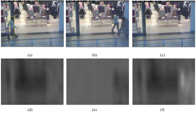
(a) (b) (c)
(d) (e) (f)
Fig. 4.3 An example of the similarity measurement by using the color histograms of target person and background image. (a) Image of a tracking target person, (b) Image of a tracking frame, (c) Background image, (d) Target appearance similarity map of the tracking frame, (e) Background appearance similarity map of the tracking frame, (f) The similarity map by combining background and target appearance models.
36 1 2 |Σ| , , , (4.12) , , . (4.13)
Fig. 4.3(d) shows the similarity map of Fig. 4.3(b) comparing with the target appearance model extracted from the person region of Fig. 4.3(a). Fig. 4.3(e) shows the similarity map of Fig. 4.3(b) comparing with the background appearance model extracted from Fig. 4.3(c). Fig. 4.3(f) shows the combines of the two similarity according to Eqs. (4.12) and (6.2). In the similarity map, the gray scale of a pixel represents the similarity of a region with the same size of the person region in Fig. 4.3(a) centered in the pixel. In Fig. 4.3(f), we can observe that the region of the target person in Fig. 4.3(b) has largest similarity.
Note that, in a particle filter, the measurement affects the selection of particles in the resampling step. The motion of the selected particles in the next frame is determined by the system dynamic model defined in Eq. (4.1). The noise W in the system dynamic model affects the distribution of the particles. Since we assume that the noise W is a Gaussian distribution, the distribution of particles forms a mixture of Gaussians in the state space. The set of Gaussian distributed particles will be placed in each important part of the state space, which will next be resampled according to the weights calculated from the measurements. All the selection and generation of particles are the characteristics of the particle filter.
4.3 Cumulative Histogram Map
37
tracker and the color histograms of the current frame and background image in the positions of these particles must be extracted. It is time-consuming to extract a large number of color histograms in an image. Since most of the regions of these particles are overlapped, many redundant calculations are spent for estimating the colors in the pixels of the overlapped regions. To reduce the redundancy, we create a cumulative histogram map (CHM) for the processing frame and background image. Then we can extract the color histogram feature for each particle in a constant time.
The CHM is similar to the integral map popularly used for extracting Haar-Like feature [20]. The map is created to cumulate the color histograms. In a region
, | , , the color histogram of a color channel can be calculated as
,
,
, (4.14)
where . is the Kronecker delta function, and is the set of colors that map into
i-th bin. According to the equation, we can define the CHM for an image as
CHM , , ,
,
. (4.15)
The CHM can be calculated recursively as
CHM , , CHM , 1, CHM 1, ,
CHM 1, 1, , . (4.16)
When we obtain the CHMs for an image, the histogram from Eq. (4.14) can be calculated as
38
Based on the modification, the time complexity for creating M CHMs for an image is , where W and H are the width and height of an image respectively and M is the number of histogram bins. The time complexity for extracting color histograms in a region is . The complexity for extracting the color histograms for N particles in an image is thus . The time complexity of histograms extraction in Eq. (4.14) for all particles in an image is , where , are the width and height of the region R. The number of bins is much smaller than . If is smaller than , the speed can be improved. According to our test results, when more particles are used, the target can be traced more precisely. In our experiments, we set the number of particles around 1000. Therefore, the speed of the particle filter-based tracker can be improved. The measurement of speed improvement will be described in the experiment result section.
4.4 Dynamic Number of Particles Adjustment
The number of particles will greatly affect the search region of the target object in an image. In general, when more particles are selected, the tracker may become less efficient but more accurate. Recently, Fox [51] proposed a method to dynamically adjust the number of particles by using the KL-distance to reduce the error. The method adjusts the number of particles to minimize the error between the true posterior and the sample-based approximation. However, the computation is costly. In a particle filter, the particles with local maximum weights are much important for the target state estimation and particle resampling. Therefore, we modify the number of particles to control the covering range in state space so that the state with the local maximum weight can be located.