A system dynamics model of fire-tube shell boiler

B. J. Huang Professor. P. Y. Ko Graduate Assistant. Department of Mechanical Engineering, National Taiwan University,

Taipei, Taiwan 10764

A System Dynamics Model of

Fire-Tube Shell Boiler

A system dynamics model of fire-tube shell boiler was developed. The derivation of the dynamics model started with a nonlinear time-variant dynamic modeling based on the transport phenomena in the fire-tube boiler. A linear time-invariant perturbed model around steady-state operating points was then derived. The

identifiable parameters tmw, Twa, K, (3, and Td were identified by using field test

data and least-squares estimation method; the coefficients C's were, meanwhile, directly predicted by using the small-perturbation relations. Empirical correla-tions of the identifiable parameters were further derived to account for the variation of parameters with operating conditions. The present perturbed model is thus semi-empirical and can describe the dynamic behaviour of fire-tube boilers over a wide range of operating conditions. The predictions of dynamic responses using the present model were shown to agree very well with the test results.

I Introduction STEAM

r

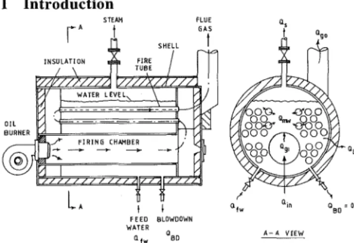
OIL BURNER I \ FEED SLOWDOWN WATER

Fig. 1 Schematic of fire-tube shell boilers

Fire-tube shell boiler or package boiler (Fig. 1) has been widely used in industries and residential areas for process heating and hot water supply. The design of fire-tube shell boilers consists of a bundle of fire tubes contained in a shell; severe boiling and evaporating processes take place outside the fire tubes and steam is generated. The heat transfer process from the combustion gas to the boiling water via the tube surface is extremely complicated as it involves combustion, radiation, convection, and boiling processes. Contributed by the Dynamic Systems and Control Division for publication in the JOURNAL OF DYNAMIC SYSTEMS, MEASUREMENT, AND CONTROL. Manuscript received by the DSCD December 4, 1988. Associate Technical Editor: P. B. Usoro.

The thermal performance of boiler is then highly nonlinear and can be significantly affected by the operating conditions such as steam pressure and flowrate, ambient conditions, excess-air quantity, degree of fuel and combustion air mixing etc. The performance can be further disturbed by the varia-tion of steam or combusvaria-tion air flow during operavaria-tion. Time-variant phenomena will also appear inevitably due to the integral effect produced by the variation of holdup water or water level in the shell side. The dynamic model of fire-tube boilers should apparently be in the following nonlinear time-variant and multi-input-multi-output (MIMO) form:

X ( o = / [ X ( r ) , U ( 0 ] Y(0 = g[X(r),U(f)].

(1) (2) The system dynamics of water-tube power boilers for the design of high performance control system of power plants has been extensively studied in the past (for examples, Chien et al., 1958; Nicholson, 1964, 1965, 1967; Anderson, 1969; Kwan, 1978; McDonald and Kwatny, 1973; Ray and Bow-man, 1976; Aleksandrov and Rassokhin, 1985). These stud-ies, however, have been mainly theoretical due to their com-plexity. The studies of dynamic models of fire-tube shell boilers have been sparse. Only a few simple lumped single-input-single-output (SISO) models for domestic fire-tube hot water heaters have appeared in literature (Lebrun et al.,

1985; Malmstrom et al., 1985; Claus and Stephan, 1985). An attempt has then been made here for developing a MIMO system dynamic model of fire-tube shell boilers.

by using the estimation methods such as generalized least-squares, instrumentvaiiables and maximum likelihood al-gorithms etc. (Hsia, 1979). The system parameters identified in this way may, however, be in large errors at operating conditions different from the one used in the identification, unless the plant is linear and time-invariant which is obvi-ously not the case for fire-tube boilers. The application of this approach is thus limited.

A model-based approach has been used here in the deriva-tion and identificaderiva-tion of system dynamics of fire-tube boil-ers. A nonlinear time-variant dynamic model was first de-rived based on the transport phenomena in the fire-tube boiler. A linearization using small perturbation around a steady-state operating point was applied and resulted in a linear time-invariant perturbed model with some well-de-fined and identifiable system parameters and some predict-able coefficients. The identifipredict-able parameters clearly possess a physical meaning and their values at various operating conditions can be identified by using test data and least-squares estimation method; the predictable coefficients are, meanwhile, a function of steady-state operating conditions and can be directly evaluated. Empirical correlations of the parameters in terms of steady-state operating conditions

were further derived to account for the variation of parame-ters with operating conditions. The present perturbed model, written in the form of Eqs. (3) and (4), is thus semi-empirical and can accurately describe the dynamic behaviour of fire-tube boilers over a wide range of operating conditions.

X(?) = A(X,U)X(f) + £(X,U)U(f) + E(X,V)t(t) (3) Y ( 0 = C(X,U)X(f) + £>(X,U)U(0 (4) II Physical Modeling and Governing Equations

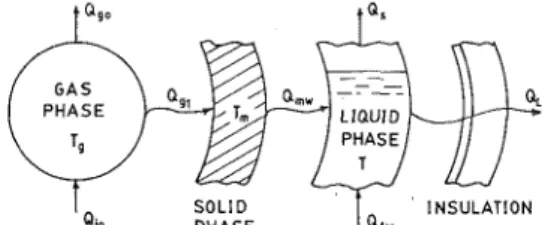
A three-node lumped model is derived here for the sake of simplicity. It was assumed that the boiler can be divided into three different phases: namely, the holdup water in the shell side as the liquid phase, the metal of the heating surface (fire tubes) as the solid phase, and the combustion gaseous product in the combustion chamber and fire tubes as the gaseous phase. Each phase was assumed to have a uniform temperature. The heat transfer between the three phases is shown in Figs. 1 and 2. The dynamic model can be obtained here by applying an energy and mass balance to each phase.

Gaseous Phase.

will lead to

An energy balance to the gaseous phase

N o m e n c l a t u r e A, = A = mw Awa =

9 =

Cg = C,n =

c

s

=

c

w

=

CO = CO, = Ht '/ h,.,„ = i = % =

theoretical air flowrate per Mg = unit fuel flowrate for

stoichio-metric combustion, Eq. (20), Mw = Nm3/kg oil

heating surface area of fire ma = tubes, m2

heat transfer surface area of way = fire tubes, m2

area used in evaluating the ms = heat transfer from the boiling

water to the ambient, m2 mw = heat capacity of fuel oil,

kJ/kg°C N2 =

heat capacity of flue gas,

kJ/kg°C 02 =

heat capacity of fire tube, kJ/kg°C

heat capacity of steam, kJ/kg°C

heat capacity of water, kJ/kg°C

volumetric concentration of gaseous CO in flue gas, % volumetric concentration of gaseous C 02 in flue gas, %

heating value of fuel oil, KJ/kg

heat transfer coefficient from fire tube to water, W/m2oC

heat transfer coefficient from

boiling water to ambient, T = W/m2oC

enthalpy, KJ/kg

enthalpy of feed water, KJ/kg Ta = QE

Qgl

Q _go

Qin QL

mass of combustion gas in the boiler, kg

mass of holdup water in the shell side, kg

mass flowrate of combustion air, kg/hr

mass flowrate of fuel oil, kg/hr

mass flowrate of steam, kg/hr

mass flowrate of feedwater, kg/hr

volumetric concentration of gaseous N2 in flue gas, %

volumetric concentration of gaseous 02 in flue gas, %

net rate of heat carried out by steam from the boiler, Watt

radiative heat transfer rate from the combustion gas to fire tube surface (solid phase), Watt

rate of energy loss from the flue gas, Watt

rate of energy input resulting from fuel combustion, Watt rate of heat loss from the liq-uid phase to the ambient, Watt

temperature of boiling water in shell side or exit steam temperature, °C ambient temperature, °C Tf Tfw T go T0 = la = <S>a = Pa = T =

temperature of preheated fuel oil, °C

temperature of feedwater, °C flue gas temperature, °C metallic fire-tube (solid phase) temperature, °C temperature of datum state, °C

absolute humidity of combus-tion air, kg vapor/kg dry air ratio of actual to theoretical combustion air flowrates, di-mensionless

density of combustion air, kg/m3

time constant for the re-sponse of fire-tube tempera-ture due to heat transfer from solid phase to boiling

water, s

time constant for the re-sponse of water temperature due to heat transfer from boil-ing water to ambient, s Superscripts

small perturbation steady-state operating con-dition

. . - „ . . . . , , INSULATION

" i n D U A C C I Q fw

Fig. 2 Schematic of 3-node model of fire-tube shell boilers

*W« X--20 x£p

dt (Af,MB), (5)

where Qjn can be evaluated by the relation (Cheng et al.,

1988; McLean and Murdock, 1972)

Qin = Qin(mf) = mfiHf+Cj(Tf-T0)y, Q can be evaluated by the relation

(6)

Qgo= Qg0(mf,ma,T)

= mf[VdCgo(Tgo - T0) + GwfAH + GwaCs(Tg0 - T0)

+ 30.5Vd(CO)] (7)

where Gw, = the water formation weight of the combustion

= .09h + .Olw, where h and w are the weight compositions of hydrogen and water in the fuel oil; Gwa = water vapor

content in the combustion air = 1.293"ya<paAB, in kg vapor/

kg oil, where ya is the absolute humidity. AH = latent heat

of water vapor = 597.5 + Cs(Tg0 - T0), kcal/kg oil; Vd = <S?aA0. The semi-empirical relation developed by Huang et

al. (1988) can be applied for Qgl, the heat transfer to the

tube walls. Qgi = Qgi(mpma,T,Tgo) = frtTAl(TG-T*) + hcAl(TG-Tl), where

r

c

* r * 4 >

?i 1 °f ' Qin Taf Qin mjlHf+Cf(Tf-T0)l laf MaCg Q,l maCS Qe + T, (8) (9) (10) (11) where fr, hc, <$>, C, n, and rw are the empirical constants;

o- is the Stefan-Boltzman constant, 5.669 x 10~8 W/m2K.

The combustion gas contained in the combustion chamber of the boiler has a very small thermal capacity in practice as compared to the boiling water to which the radiative and convective heat Q x will be transferred. The energy storage

rate due to the thermal capacity effect of the combustion gas can then be relatively very small too as compared to

Qin and Qgl. This is due to a rapid chemical combustion

process with heat generation rate Qin and a fast heat transfer

process <2„j. For the sake of simplification, the thermal ca-pacity effect of the combustion gas is neglected here. This may cause a larger error in predicting the flue gas tempera-ture response since the flue gas loss rate Q may be closely related to the energy storage rate of the combustion gas.

This, however, may not be too serious since Qg0 is relatively

small as compared to Qin and Q x and the efficiency control

of a boiler is of the major concern in many applications. A quasi-steady approximation can therefore hold and the en-ergy equation for the gaseous phase becomes

*£go x~in x--g (12)

Solid Phase., Applying an energy balance to the solid

phase will lead to

M,„C„ dT, '" "' dt

where the last term h,

- Qgi *lmwAmw{Tm T) (13) mWAmw(Tm " T) represents the heat

convection from tube surface to boiling water.

Liquid Phase. Applying an energy balance to the liquid

phase for zero blowdown (QBD = 0) will lead to

dt [MWCW(T - T0)} = hmvAnm{Tm -T)-QE-QL (14)

where QE is the net rate of heat carried out by steam from

the boiler; QL represents the rate of heat loss from the liquid

phase to the ambient, i.e.,

QE = ms(is ~ '<,) - mw('/w - U (1 5)

QL = hwaAwa(T-Ta) (16)

where i0 is the enthalpy of water at datum state.

Stoichiometric Relation of Gaseous Phase. In addition

to the energy and mass balance relations, a stoichiometric relation for the chemical combustion process in the boiler can be derived for the flowrate of combustion air (Cheng et al., 1983; McLean and Murdock, 1972),

where ma = 9amfAa, <|>a(l + 1.61-ya)A0) in N m3/ k g o i l 21

K = —

2 1 - 7 9 O2-0.5CO\ N-, I (17) (18) (19) AQ = .0889c + .267 h--\ + 0333s, in Nm7kg oil (20)

AD is the theoretical combustion air flowrate per unit fuel

flowrate for stochiometric combustion, where c, o, and s are, respectively, the weight concentrations of carbon, oxy-gen, and sulfur in the fuel oil.

The above modeling results in the governing equations of fire-tube boilers, i.e., Eqs. (12), (13), (14), and (17). I l l S m a l l P e r t u r b a t i o n s

Using the small perturbations around a steady state:

Qin{t) = Qin + j 2 / „ « ; Qgoit) = Qg„ + Qg0{t)\ QE(t) = QE + QE{t); 7X0 = 7^+ f{t); TJf) = Tn±+ fm(t); mw(t) = mw + mjt)\ ms(t) = ms + ms(t); Qgl(t) = Qgl + Qgl(t), a perturbed

balance relation dMw/dt - mw - ms and neglecting the higher-order effects, where Qgo - Qin Qg\

df

m

.

T

-f"

+ ( P + 1 ) f = P f

'""

P

^

i = QE +Cw{mw-ms){T-T0 )-(21) (22) (24) MC„ K„ = -mw -mw l h A llmw mw 7wa h MWCW A wa wa h A . mw mw "wiAv

The higher-order terms essentially represent the integral effect due to the variation of water holdup in the shell side and the unbalance of steam and feedwater flowrates. This makes the boiler to behave like a nonlinear time-variant system. However, for safety reason, the water level in the fire-tube boiler is allowed to vary only within a finite range, usually within 2 cm. The variation of holdup water volume is therefore small as compared to the total holdup volume. The integral or time-variant effect can then be neglected by using small-perturbation approximation. In other words, the holdup water volume in the shell side can be assumed to be approximately constant.

Equations (21) to (23) are the small-perturbation equations in terms of the perturbed heat flows Q's which are not the primary system inputs. From the point of view of system dynamics, the direct or primary inputs of the boiler are the fuel oil flowrate m^ the combustion air flowrate ma and the

feedwater flowrate mw. The measurable outputs are the water

or steam temperature in the shell side T, the flue gas tempera-ture T and the oxygen concentration 02 of the flue gas,

the steam load ms, meanwhile, acts as a disturbance input

to the boiler. The model obtained so far is apparently nonlin-ear in terms of these primary inputs since the heat flows Q ,

Qgl, and QE appearing in the above equations are nonlinear

functions of these input variables. Linearizations using small perturbation around a steady state are further required.

Applying small perturbation to Eq. (6) and using a first-order approximation will lead to

Qin Cifmf (25) where Clf = if~\d *Qi, _H f + CATf-TD). "•f'o

Taking small perturbation of Eq. (15) will lead to

QE = Cewmw + Cesms + CeTf, ( 2 6 )

where

c

-

s

(^d

0=

~

iifw

~

io)

The subscripts "o" denote the derivative in respect to a steady-state point. If the datum state is chosen as the feedwa-(23) ter state at 7 ^ , then T0 = 7^,; i^ = i0; and Cew = 0 and we

obtain

QE = Cesms + CeTf. ( 2 7 )

Similarly achieved here for the flue gas heat loss Qgo is

(28) Qgo = Cof"ia + Coama + C f where C°f= ( l ^ )0 = V"C^T„o - T0) + GwfAH + GwaCs(Tgo-To) + 30.5VdCO, fdQ„„\ C„„ m, -C" " " ' ^ f = ~ f ^ - T0)+1.293ya-tC,(Tt0 - To) 3 0 . 5 -Pa •CO, C

° ^ ( I H =™fl

V

<t

CS

o + G

wf

C

s +

G

wa

C

s

].

^ go'o

For the radiative heat transfer Qgl, small perturbation on

Eq. (8) and using quasi-steady approximation yields

2 , 1 = Crf™f + C>a + Cj + Crgfgo, (29) where C „ 3 Cr. Al(4frcrTG + hc)[FfieCif/Al fiQgi\ -(^/mf){\-FaM Al(4fr<rTG + hc)(4>e/ma)(l - FJ ~f \dmfJ0 4fr<r(TGFfi-TlFrw) + hc(Ffi-Frw)-l a™„ L 4frv(T3GFfi - T\FrJ + hc(Ffi - Frw) - 1 C „T —

J*Q*

37 rg

Ur„

A^AfaTl + hJ 4fMT3GFfi - T\Frw) + he(Ffl - Frw) - 1 C,„ = - A , ( 4 / , a 7 * + / y 4fru{TGFfi - T\Frw) + hc(Ffi - Frw) - 1 Taf~T AiF, af Faf- — ' ^ / ; -(P - ! Frw~rw •af Qin + nC\ Qsi\n -T G S T + ^ QgiTaf-T0 Qin Taf Qin "f maCg maCg maCg

For the combustion air, small perturbation to Eq. (17) the state-space model is then obtained here in the form of yields, neglecting the effects of CO concentration since it Eqs. (3) and (4) with

is usually very low in commercial boilers:

where C*-\dr, ™a = Cmf™f + Cmo°2< (30) / P + 1 + KCeT _P_\ A(X,U): lf'o

c„

pf l[ ^ + ( 4 >a- i ) A0] 79pamfA0$a ^ 2I0 2lN2-19(O2-0.5CO)' \ P+K(CrT-RTCrB) -1_ BT T " mw mw (40) B(X,U)

All the coefficients C's are a function of the steady-state operating conditions and can be directly evaluated. IV System Dynamic Model

The state-space model is derived here first. The states are defined as KCW(T-Tfw) K{Crf+RfCrs) K(Cra + RaCrs) B T B T r* mw r1 mw C(X,U): / i o\ -RT 0 0 0 x{ = T x2 = Tm. 0 (31)

The above small-perturbation relations are then substituted into Eqs. (21)-(23) to lead to

B + 1 + KCe -x, + • D(X,U) E(X,U) R f 0 0\ -R„ 0 L. 1 T - ^ 9 T T wa wa -KjC^-CJT-T^)]] T wa o (41) (42) (43) (44) K[Ces-Cw(T-T0)] KCW(T-T0) m„ m. [S + K(CrT - RTCrg)] 1 (32) B T X \ X'y

Taking Laplace transform of Eqs. (3) and (4) will lead to

Y(s) = G(j)U(j) + W ( j ) f ( j ) , (45) The MIMO transfer-function plant model G(s) is then

K(Crf+RfCrs) _ K(Cra - RaCrg) _ + „ —Ui-mf+ z: &~m„ S T ' B T " mw r* mw T„„ = -RTxl + Rfiht - RJna C. go On (33) G ^ ) = C ( r f - A r1B + D Ka„ 'mo ^mo (34) (35) where aas + 7 i ^ + 7 2 a.0s + 7 i ^ + 72 (46) K(wBs + w,) \ Crn + C h A "'wa wa R- Ci f - Co f -C f~ c„„ + c a0s +yxs + y2 r + R -RTKa0 -R TK(w0s + wx) 7 a0J2 + 7 ^ + 72 0 rl- ₍₄₇₎ / og R„

c + c

. o g * W g RT ~ C _{rT where} C + C

The state vector X, the manipulating input vector U, the output vector Y, and the disturbance input vector T are defined as (36)

x =

U s \1 m> ma \< / f * . . fgo (37) (38) yl = al + CeTK'Tmw 72= 1 +{CeT-CrT+CrgRT)K a = T T o mw wa a , = ( l + B ) Tm l v + Tw a fo= Crf+CrgRf ao = Cra ~ Crg^a Qo = Jmw\-Cw(T ~ Tfw) ~ C« ]

e,

o-,

T = (ms), (39) CW(T - Tfw) - Ces ^\ = -Cw(T- Tfw).

The plant disturbance model W(s) can be written as

/ K^s'+BJ \

a0s2 + yxs + y2 RTK(QoS + 6,) a0s + 7,5 + 7;

0

The resultant MIMO plant model for a fire-tube shell boiler can be seen to be 3- x 3. The interactive or cross effects between the inputs and outputs are present since the plant transfer function G(s) is nondiagonal. The variation of plant dynamics with the steady-state operating points can clearly be seen from the present model.

The system dynamic model of fire-tube boilers developed above is based on the physical modeling with several simpli-fications. Some unmodeled dynamics must then exist which may reflect to the time delay or high-order effects. The time delay effect may not be negligible for the temperature response of boiling water in the shell side T(t). A modifica-tion is thus required.

Assuming that the time delays for the boiling water tem-perature response f(t) with respect to the manipulating inputs U ( 0 and disturbance input F(t) are the same, i.e., id, then

the first raw of G(*) and W(s) have to modified by multi-plying a delay term e~^dS. This assumption can

approxi-mately hold since the dynamic responses Y (steam and flue gas temperatures, f and f and flue gas concentration 62)

due to the disturbance input T (steam load ms) and the

manipulated input U (mass flowrates of fuel, air and feedwa-ter, rhp ma,mw) are produced by a heat transfer through the

holdup water in the shell with a large thermal capacity and are therefore approximately in the same order of magnitude. With this consideration, the system dynamic model of fire-tube boilers finally becomes

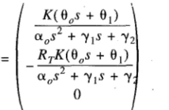
G(s) = n <V + 7 ^ + 72 -RTKfB Ka^i Ke-"d(Wos + Wl)\ <V +7i* + 72 a0s + 7 ^ + 72 + Rt -RTKa0 -C, mL a0s + 7 ^ + 72 1 -/?„ <V +7i* + 72 ~RTK(w0s + w1) W ( J ) = r IK{% s + e ^ e - " ^ a0s2 + yxs + y2 RjKjQ^ + e,) a0s2 + yxs + y2 0 a0s + yls + y2 0 \ / (49) (50)

The schematic of system dynamic model in state-space and transfer-function forms is presented in Fig. 3.

Equations (49) and (50) represent the system dynamic model of fire-tube boilers in which all the coefficients in-volving C's can be directly predicted by the small-perturba-tion relasmall-perturba-tions described in Secsmall-perturba-tion III; Tmiv, T K, (3 and

G(s) W(s) + *• + B D 4 x₊ i>^

\y

A X _c + ^

Fig. 3 System block representation of fire-tube shell boilers, (a) Trans-fer-function model; (b) state-space model

id are the system parameters which can be identified using

field test results and thus are referred to as "identifiable system parameters."

V P a r a m e t e r E s t i m a t i o n

1 Experimental Setup. A half-ton fire-tube shell

boiler installed in the laboratory was used for the experiment in the present study. Refer to the recent paper of Huang et al., (1988) for the specification of the test boiler. The empirical constants defined in the radiative heat flux relation Qgl, Eq.

(8), for this test boiler a r e /r = 0.38567; hc = 13.99 W / m2 oC ;

<$> = 1123.09°C; C = 865.11; n = -0.0019912; rw = 3.078 x

10"4 m2° C / W (Huang et al., 1988).

Three T-type thermocouples were installed in the shell side to measure the average boiling water or steam tempera-ture in the shell side; among them, two were immersed 5 and 10 cm under the water level to detect the water temperature in shell side; and the other one was 10 cm above the liquid level to measure the water vapor temperature. The average value of these three temperatures was taken as the boiling water (liquid phase) temperature. Other four T-type thermo-couples were installed in the chimney, feedwater storage tank, fuel line of the burner, and ambient to respectively measure the temperatures of flue gas, feedwater, fuel oil, and ambient. The precision error is estimated to be ±0.1°C. The pressure in the shell side was measured by a Endevco 8510-200 pressure transducer installed at the steam exit of the boiler. The flowrates of the feedwater and fuel oil were respectively measured by a MK-508 turbine flowmeter and a OVAL EC-250 gear-type flowmeter, both with pulse output signals. OVAL EC-250 has been calibrated to give a sensitiv-ity of .01714 kg/pulse with an uncertainty of ±1.6 percent. The sensitivity for MK-508 is .00151 kg/pulse with an uncertainty of ±2.9 percent. The flue gas compositions were measured by a gas analyzer of Energy Efficiency System Co. which gave an uncertainty of ±0.3 percent for 02, ±2

percent for CO gas and ±10 percent for C 02 gas. The steam

flowrate was measured by an orifice meter which was com-posed of an orifice plate and two pressure transducers (Ya-matake Honeywell piezoelectric transducers).

The dynamic data were taken using a data acquisition system AD700S. All the analog signals of the transducers and sensors were first picked up by a HP 3456A digital

voltmeter with GPIB output connected to IBM PC; the pulse output signals of the turbine flowmeters were, meanwhile, counted by a counter card (AD50120) within AD700S. Soft-ware compensation was used with a cold junction compensa-tion card (AD50010T) for temperature measurements. Two 10-channel multiplexers (AD50010) were used for multiple channel measurements. The maximum reading rate of the data acquisition system was 330 reading/sec. The sampling time interval for the present experiment was 3 seconds.

The feedwater flow was regulated by a water level relay control system. Since the laboratory boiler was equipped with an automatic burner, for safety reason, the primary system inputs (flowrates of combustion air and fuel oil) could not be arbitrarily adjusted in the present experiment. Only the nozzle of the burner could be changed here to vary the oil flowrate. For a given nozzle and a fixed setting of excess air, the burner is automatically operated. It is due to this restriction that the primary inputs (mf, ms,mw, ma) cannot be chosen as the input signals for system identification in the present study. Instead, the secondary input signal Qgl and £ were used.

2 Input Signals. Combining Eqs. (22) and (23), while taking into account the time delay, will lead to

-S(k) T(s) Ke-S"i ^mw^Wa(S+Pl)(S+P2) 2 , i (51) Ke-">i(s + ze •£ = GT(s)Qgl(s) + WT(s)Us), Ke ~"d (52) GT{s) where P\ ze = + p2 T T mw 1/Tm wand

J

s + ( l + P ) Tm w + Twa T T _{' mw wa} p mw 'wa^-P 1 + p2) p

-0(s+p

2

y

PiPi = T - T _{mw wa} 1 T T mw wa (53) (54) The secondary input signal Q t can be evaluated by measur-ing Qin and Q and by using Eq. (21); |_can be evaluated by Eq. (24) and the relation QE = QE - QE. Both the input signals Qgl and I were mainly produced by a cyclical opera-tion of a feedwater pump due to the relay on/off during the water level control. It was found in the present experiments that they were approximately persistently exciting over the frequency range of 0 ~ 0.3 Hz. From the above derivations, the parameters to be determined are K, Td, ze, px and p2 which corresponds to the system parameters K, id, rmw, twa, and (3.

Equation (52) can be discretized for digital signal pro-cessing by z-transform to yield

T{z) ~nd B(z )A A(z'1) fi e,(z) + C(z-1) -A(z'1)

Uz)

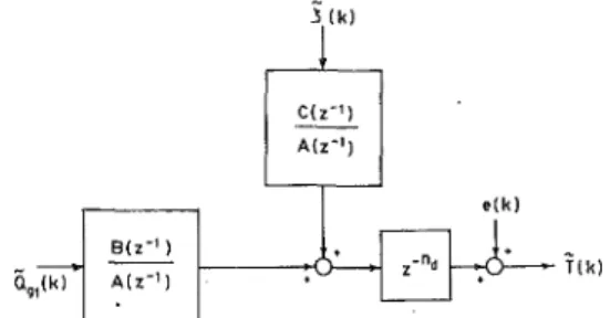
(55) a„(k) B i z " ' ) A l z - ' l C(z"') A(z"') z-n- T(K)

Fig. 4 System block diagram for parameter identification

A(z with the ( -1) •= \ +axz x + a2z !; B(z~ C(z-1) = c1 + c2z-1; ;orresponding coefficients « i « 2 * i ci c2 = -(rx + r2) = rxr2 Kplp1(r2- /-,) P\ 'Pi = -KtmwPlPl K. Pir2-Pirx + ze{n l) = bxZ-1; -r2) (56) (57) P\ -Pi where

where rx and r2 are the z-poles of the plant; px and p2 are s-poles.

3 Signal Pretreatment and Parameter Estimation. Pretreatment or prefiltering before system identification is required since the testing signals could be corrupted by internal and external disturbances or noises. The internal disturbance was mainly generated by the severe agitation effect of the boiling water and evaporating process in the shell side (i.e., an unmodeled dynamics) and imposed on the response of steam or boiling water temperature. The external noises were essentially the measurement noises. Both kinds of disturbances and noises were in high-fre-quency range, as compared to the system response. A low-pass filtering for the testing signals was therefore applied. The following third-order smoothing filter F(z~l) was used in the present study,

1 i

(58)

i = - i

where uk andyk are, respectively, the input and output signals of the filter. The discrete-time model in terms of the filtered signals then becomes, from Eq. (55),

A{q-X)f*(k) = B{q-l)Q*gl(.k - nd)

+ C(q-1)i*(k-nd) + e(k) (59) where e(k) is the residue; A(q~l), B(q~l) and C(q~l) are the estimates of the system parameters in terms of backward shift operator q~l\ f*(k), Q*gl (k - nd) and l*(k - nd) are the filtered signals by the filter F{z~l). That is,

f*(k) = F(q~l )f (*); Q*gl(k - nd) = F(q-l)Qgl(k - nd);

l*(k-nd) = F{q-1)l(k-nd) (60) The system block diagram for parameter identification is

shown in Fig. 4.

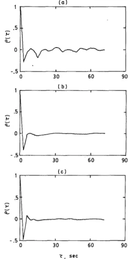
ad- fig-m,=

Model fitting results, (a) m, =J4.6 kg/hr, Ps =^3.8 kg/cm2; (£>) .0 kg/hr, P, = 5.1 kg/cm2; (c) m, = 37.9 kg/hr, Ps = 7.3 kg/cm2

The least-squares method was used in the present study for estimating the system parameters using Eq. (59). The dynamic data was seen to closely follow the predicted values as shown in Fig. 5 for some of the results.

The parameter estimation is well known to be unbiased if the residue e(k) is a statistically independent random process (Hsia, 1979). The whiteness of the residue can be examined by using the normalized autocorrelation function of e{k), p(«).

p(w) ₍₆₁₎

where Ree(n) is the autocorrelation function of the residue. The residues e(k) for various operating conditions being quite close to a white signal can be seen from Fig. 6.

The present tests were run at six different operating condi-tions with the fuel flowrate ranging from 14.6 to 37.9 kg/

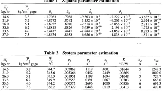
hr; the water flowrate ranging from 181 to 465 kg/hr; the steam pressure ranging from 3.8 to 7.3 kg/cm2gage. The

identified system parameters in terms of ax, a2, bx, cx, c2 are presented in Table 1. The steady-state gains K were determined by the relation derived from Eq. (14),

K = 1 T-T„

^wcAwa Qgl ~ Ql

(62) From the above results, the parameters Pi,p2>nd<ze(=l/ Tmw), Twa were determined and from which (3 can be evaluated by Eq. (54) using ze, Twa, px, and p2. The final results are presented in Table 2. All the identifiable system parameters, T „ , Jwa, (3, Td, and K, appearing in the state-space equations, Eqs. (40) to (44) and Equations (49) and (50), thus can be determined from these results.

4 Empirical Correlations of Parameters. The param-eters pl,p2, nd, ze{= 1/T„W), Twa can be seen to vary with the

steady-state operating conditions which can be essentially

Fig. 6 Whiteness of residue, (a) m, =_14.6 kg/hr, Pn := 3.8 kg/cm2; (b)

m, = 26.0 kg/hr, P, = 5.1 kg/cm2; (c) m, = 33.6 kg/hr, P, = 6.2 kg/cm2

represented by the fuel flowrate m* and the steam pressure

Ps. The approximate empirical relation was derived as:

t|i = C'mjPl, (63)

where i|/ represents the parameters pv p2, nd, ze, Tmw. The

identified results as shown in Table 3 and Fig. 7 have been obtained by using least-squares fitting.

5 Model Verification. The dynamic model previously developed can be verified by substituting the identified pa-rameters Tmw, Twa, K, (3 and rd and the coefficients C's into the MIMO model, Eqs. (32) to (35) or Eqs. (3) and (4), for system simulation and comparing with the test results. The parameters tmw, iwa, K, (3 and Jd were evaluated using the empirical relation, Equation (63) and Table 3; the coeffi-cients C's were, meanwhile, calculated by the small-pertur-bation relations derived in Section ffl.

The test data can be seen from Fig. 8 to coincide very well with the simulations for the response of steam (or boiling water) temperature f(t). The simulation results for the flue gas temperature are in a larger error (Fig. 9). This is due to the fact that the present modeling used the quasi-steady approximation and ignored the thermal capacity effect in the gaseous phase. However, the error in predicting the flue gas temperature response is tolerable.

Table 1 Z-plane parameter estimation mf kg/hr 14.6 21.9 26.0 33.6 33.6 37.9 P, kg/cm2 gage 3.8 5.2 5.1 6.2 4.0 7.3 " I -1.7063 -1.8572 -1.6922 -1.8818 -1.4437 -1.8674 ai .7088 .8592 .6940 .8826 .4447 .8683 * i -9.303 x 10"9 1.152 x 10"8 -2.514 x 10-8 -5.639 x lO"10 -1.884 x 10"8 6.656 x 10"10 ^1 -2.222 x 10"9 -9.205 x 10"10 -3.856 x 10"9 -2.191 x 10'9 -1.059 x 10"8 -1.838 x 10~9 c2 ' -3.632 x 10"11 2.924 x 10"10 2.211 x 10"9 1.778 x 10"9 8.233 x 10"9 1.571 x 10""9

Table 2 System parameter estimation mf kg/hr 14.6 21.9 26.0 33.6 33.6 37.9 Ps kg/cm2 gage 3.8 5.2 5.1 6.2 4.0 7.3 Ts °C 344.7 345.6 345.3 349.9 344.2 356.2 P\ s"1 .002868 .005366 .001951 .002553 .000575 .002329 Pi s"1 .1119 .0452 .1198 .0391 .2696 .0448 ze s-1 .4001 .2449 .1694 .0667 .1080 .0519 K °C/W .01644 .00865 .01048 .00703 .00836 .00413 "d

a

5 1 3 3 6 4 T wa S 1247.3 1009.0 724.7 668.6 697.3 498.0

Table 3 Semi-empirical correlations of system parameters.

- simulated ... measured feedwater flow signal (ON/OFF)

* c Pv s p2, s" ze, s K, °C/W nd, A T«.0.s ">/• .02878 .36795 147.90 .37991 1.6988 .00014 kg/hr; -2.4041 1.3888 -1.7757 -.7084 1.0706 -.7600 P,- kg/ 3.2525 -3.7238 -.7171 -.9099 -1.7663 -.2470 cm gage 004 002 • Pt : , 0 ' s" ', 1 1 o .002 40 20 ' ' ' ' 1 ^ • s 0 ,' 0 ,' 500 1000 1500 0 10 20 FITTED, eqn(63)

Fig. 7 Fitting of empirical relations for system parameters

? h" 1

f .

J

-&—-'; • j J \ i J1

j/|\i/i

fr ! T !

1 A

Vl/I

If

i i i

\ If

t_.

K'"1 A r~ •'

v/iVi/V

/ /

T f ; f

X i k

W

T |-

w

Fig. 8 _Model verification for_steam temperature response, (a) m, = 21.9 kg/hr, P„ = 5.2 kg/cm2; (b) m, = 33.6 kg/hr, P, = 6.2 kg/cm2

- simulated ... measured feedwater Bow signal (ON/OFF)

Fig. 9 Model verification for flu<2 gas temperature response, (a) m, •• 33.6 kg/hr, P„ = 6.2 kg/cm2; (b) m, = 37.9 kg/hr, Ps = 7.3 kg/cm2

VI Discussions in Table 2 to be due to a heat transfer from the metallic _{tube (solid phase) to the holdup water in the shell side. The} The time constant for the response of solid phase tempera- time constant Tmw (= 1 lze) decreases with an increasing fuel ture can be seen from the estimated parameters presented firing rate m, and operating pressure Ps and is in the order

of 2 to 20 s. This is due to the fact that the boiling phenome-non in the fire-tube boiler is possibly film boiling. The metal surface temperature tends to rise as the heating rate (i.e. fuel firing rate) increases. This causes the convective heat transfer coefficient hmw to decrease. This makes the time constant Tmw = ^mC„//!mivAmw increase.

The time constant Twa for the response of liquid phase due to the heat loss from the holdup water in the shell side to the ambient increases_with increasing fuel firing rate rrij-and operating pressure Ps'and are in the order of 8 to 20

minutes. This is mainly due to the fact that a higher fuel firing rate and operating pressure result in a higher agitation effect of the boiling water (liquid phase). This in turn, in-creases the overall heat transfer coefficient hwaAwa and thus reduces the time constant jw a.

The system dynamics of the fire-tube shell boilers is of second order as seen from the present study. Two s-poles,

p{ and p2, and one s-zero, ze exist. The results presented in Table 2 further show that the magnitudes of s-pole p2 and s-zero ze are in the same order; the s-pole pl is, meanwhile, smaller than p2 by an order. A order reduction to a first-order model is then possible (Franklin et al., 1986).

Three sources of errors exist in the system identification: the time-variant or integral effect due to the variation of holdup water level in the shell side, the internal disturbance induced by the agitation of boiling water, and the assumption of lumping in the modeling. However, the variation of holdup water was relatively small (<2 percent) as compared to the total holdup water in shell side. The internal distur-bance was filtered out by a low-pass smoothing filter F(z~}). The assumption of lumping can be corrected by adding a time delay term in the model. The resultant error in the parameter estimation can then be negligible. This was proven by the comparison of the test results with the simulation by using the present model.

The cross or interactive effects between system inputs and outputs are noticeably taken into account in the present MEMO dynamics model. The effects of parameter variations on the plant dynamics is one of the sources causing plant uncertainty as in regard to the issue of robust control using linear controller design procedures. The parameter variations may result from the variation of operating conditions. The dynamics model identified in the present study can be used to accurately estimate this type of plant uncertainty and thus it is applicable to the design of various robust control systems.

VII Conclusion

A system dynamics model of fire-tube shell boilers has been developed here by using a model-based approach. The derivation of the dynamic model started with a nonlinear

time-variant dynamic modeling based on the transport phe-nomena in the fire-tube boiler. A linear time-invariant per-turbed model around steady-state operating points was then derived. The identifiable system parameters T„W, Twa, K, |3,

and id were then identified by using field test data and v

least-squares estimation method; the coefficients C's were, meanwhile, predicted directly using the small-perturbation relations. Empirical correlations of the identifiable parame-ters were further derived to account for the variation of parameters with operating conditions. The present perturbed model is thus semi-empirical and can describe the dynamics behaviour of fire-tube boilers over a wide range of operating conditions. The predictions of dynamic responses using the present model were shown to agree very well with the test results.

Acknowledgment

The present work was supported by the National Science Council of Taiwan, the Republic of China through grant no. NSC77-0401-E002-17.

References

Aleksandrov, V. V., and Rassokhin, G. N., 1985, "Predicting the Dynamic Instability of Oncethrough Sodium-Water Steam Generator," Thermal Eng., Vol. 32, No. 11, pp. 62-64.

Anderson, J. H., 1969, "Dynamic Control of a Power Boiler," Proc. IEE, Vol. 116, No. 7, pp. 1257-1268.

Chen, Y. C , Chuan, S., and Lee, M. Y., 1983, "A study on calculation method of boiler efficiency," Technical Report No. EMR-024, Energy and Mining Service Organization, Industrial Technology Research Institute, Taiwan.

Chien, K. L., Ergin, E. I., Ling, C , and Lee, A., 1958, "Dynamic Analysis of a Boiler," Trans. ASME, Vol. 80, pp. 1809-1819.

Claus, G. and Stephan, W., 1985, "A General Computer Simulation Model for Furnaces and Boilers," ASHRAE Trans, Vol. 91, Part 1, CH-85-02 NO. 1. Doebelin, E. O., 1983, Measurement System: Application and Design, McGraw-Hill, New York, NY.

Franklin, G. F., Powell, J. D. and Emami-Naeini, A. 1986, Feedback Control

of Dynamic Systems, Addison-Wesley.

Hsia, T. C , 1979, System Identification, Lexington Books, Lexington, Mass. Huang, B. J., Yen, R. H. and Shyu, W. S., 1988, "A Steady-State Thermal Performance Model of Fire-Tube Shell Boiler," ASME J., Gas Turbines and

Powers, Vol. 110, pp. 173-179.

Kwan, H. W., 1970, "A Mathematical Model of a 200 MW Boiler," Int. J.

Control, Vol. 12, No. 6, pp. 977-998.

Lebrun, J. J., Hannay, J., Dols, J. M. and Morant, M. A., 1985, "Research of a Good Boiler Model for HVAC Energy Simulation," ASHRAE Trans, Vol. 91, Part 1, CH-85-02 No. 2.

Malmstrom, T. G., Mundt, B., and Bring, A. G„ 1985, "A Simple Boiler Model," ASHRAE Trans, Vol. 91, Part 1, CH-85-02, No. 3.

McDonald, I. P. and Kwatny, H. G., 1973, "Design and Analysis of Boiler-Turbine-Generated Controls Using Optimal Linear Regulatory Theory," Trans.

IEEE, Vol. AC-18, No. 3, pp. 202-209.

McLean, W. G., and Murdock, I. W., 1972, "ASME Power Test Code Steam Generating Units PTC 4 . 1 , " ASME, New York.

Nicholson, H., 1964, "Dynamic Optimization of a Boiler," Proc. IEE, Vol. I l l , No. 8, pp. 1479-1499.

Nicholson, H., 1965, "Dual-Mode Control of a Time-Varying Boiler Model with Parameter and State Estimation," Proc. IEE, Vol. 112, No. 2, pp. 383-395.

Nicholson, H., 1967, "Integrated Control of a Nonlinear Boiler Model," Proc.

IEE, Vol. 114, No. 10, pp. 1569-1576.

Ray, A., and Bowman, H. F., 1976, "A Nonlinear Dynamic Model of a Once-Through Subcritical Steam Generator," ASME JOURNAL DYNAMIC SYSTEMS, MEASUREMENT, AND CONTROL, Vol. 98, pp. 332-339.