門檻向量誤差修正模型在金融市場之運用

全文

(1)國立交通大學管理科學系博士論文 No. 20 門檻向量誤差修正模型在金融市場之運用 The applications of the threshold vector error correction model in financial markets. 研究生：魏伶如指導教授：鍾惠民. 教授. 許和鈞. 教授. 中華民國九十五年五月.

(2) 國立交通大學管理科學系博士論文 No. 20 門檻向量誤差修正模型在金融市場之運用 The applications of the threshold vector error correction model in financial markets 研究生：魏伶如研究指導委員會：王耀德. 教授. 謝國文. 教授. 鍾惠民. 教授. 許和鈞. 教授. 指導教授：鍾惠民. 教授. 許和鈞. 教授. 中華民國九十五年五月.

(3) 門檻向量誤差修正模型在金融市場之運用 The applications of the threshold vector error correction model in financial markets. Student：Ling-Ju Wei. 研究生：魏伶如指導教授：鍾惠民博士. Advisors：Dr. Huimin Chung. 許和鈞博士. Dr. Her-Jiun Sheu. 國立交通大學管理科學系博士論文 A Dissertation Submitted to Department of Management Science College of Management National Chiao Tung University in Partial Fulfillment of the Requirements for the Degree of Doctor of Philosophy in Management May 2006 Hsin-Chu, Taiwan, Republic of China 中華民國九十五年五月.

(4) 門檻向量誤差修正模型在金融市場之運用. 研究生：魏伶如. 指導教授：鍾惠民博士許和鈞博士. 國立交通大學管理科學系博士班. 摘. 要. 本研究使用門檻向量誤差修正模型(threshold vector error correction model)，探討兩個領域中，衍生性金融商品與其標的物價格間之動態關係。第一個主題，是有關於美國存託憑證(ADRs)與其標的股價格間的動態關係；第二個主題則是有關於交易成本的減少對於臺灣期貨交易所(TAIFEX)電子現貨與電子期貨間領先落後之關係。在第一個主題中，本研究使用的近年來所發展的門檻共整合架構，著手估計存在於美國存託憑證(ADRs)與其標的股價格間動態關係，本實證結果支持美國存託憑證 (ADRs)與其標的股價格間存在非線性均數復歸(mean-reversion)的現象；而在極端狀態 (extreme regime)下，門檻向量誤差修正模型中誤差修正項的係數估計顯示出較線性向量誤差修正模型所估計的係數大；在美國存託憑證(ADRs)與其標的股價格間的短期動態效果，在典型狀態(typical regime)與極端狀態(extreme regime)之間是有顯著的差異。在第二個主題中，本研究估計臺灣期貨交易所電子現貨與電子期貨之間長期均衡、短期動態關係，並檢視其價格間是否存在著非線性的關係。本研究使用臺灣期貨交易所(TAIFEX)電子現貨數與電子期貨之間的價差，於調降交易稅後進行線性模型與非線. i.

(5) 性模型預測能力的比較。於民國 89 年 5 月 1 日後，臺灣期貨交易所(TAIFEX)的期貨交易稅由千分之零點五調降為千分之零點二五。研究發現在減稅後，臺灣期貨交易所 (TAIFEX)電子期貨扮演一個價格發現的角色；而且門檻值也隨之降低；在樣本外的預測比較顯示門檻向量誤差修正模型的結果是較線性向量誤差修正模型佳。. 關鍵詞：門檻、向量誤差修正模型、非線性均數復歸、共整合、美國存託憑證、交易成本. ii.

(6) The applications of the threshold vector error correction model in financial markets. Student：Ling-Ju Wei. Advisors：Dr. Huimin Chung Dr. Her-Jiun Sheu. Department of Management Science National Chiao Tung University. ABSTRACT This dissertation employed the threshold vector error correction model (VECM) to investigate (1) the dynamic relationship between the prices of American Depository Receipts (ADRs) and their underlying stocks and (2) the effect of transaction cost reduction on the lead-lag relationship between the Taiwan Futures Exchange (TAIFEX) Electronic Index and Futures. First, this study set out to estimate the dynamic relationship that exists between the prices of ADRs and their underlying stocks using a number of recent developments of the threshold cointegration framework. The empirical results support the notion of nonlinear meanreversion of the prices of ADRs and their underlying stocks. The estimated coefficients of the error correction terms in the ‘extreme’ regime appeared to be larger than those in the linear VECM. The short-run dynamic effects of ADRs and UND prices showed significant differences between ‘typical’ and ‘extreme’ regimes.. iii.

(7) Second, this study explored the dynamic relationship that exists between prices of the TAIFEX Electronic Index and Futures, in both the short-run and the long-run, and examined the possible nonlinear relationship between them. Using prices of the TAIFEX Electronic Index and Futures, this study carried out a number of forecast comparisons of the out-ofsample predictability of linear and nonlinear models after TAIFEX Electronic Futures reduced the transaction tax from 5 basis points to 2.5 basis points on May 1, 2000. Results showed that the TAIFEX Electronic Futures plays a dominant price discovery role. The threshold value decreased after a transaction tax reduction. An out-of-sample comparison was conducted, which showed that the forecast results of the threshold VECM were more reliable than those of the linear VECM.. Keywords: threshold, vector error correction model, nonlinear mean-reversion, cointegration, ADR, transaction cost. iv.

(8) 致. 謝. 終於到了可以寫致謝的階段了，真是興奮不已。四年的博士班生涯，即將劃上句點。回首來時路，點滴在心頭，心中真是百感交集，五味雜陳。. 博士學位的取得，首先要感謝恩師鍾惠民老師與許和鈞老師的細心指導，對於資質愚昧的我，給於極大的幫助與鼓勵，要不是鍾老師的耐心教導，我是很難拿到學位的；另外，也要感謝口試委員王耀德教授、謝國文教授、林美珍教授和謝文良教授所提供的寶貴意見，使本論文更臻完備周詳，在此獻上我最真誠的敬意與謝意。. 要感謝增展、Curtis、Cindy、Burt 你們的幫忙，由於你們無私的支持，才能使我順利的取得學位；此外，也要謝謝這四年期間和我ㄧ起談心與歡笑的同窗摯友，一些新、舊同事與眾多的好友，族繁不及備載，我就不一一提及了，在此，誠摯地謝謝你們。這一路上走來真的有太多貴人與幸運，使我得以順利的完成學位；要感激的人實在太多了，感激你們熱情的參與，伴我走過生命中的起落，人生因為有你們，更顯燦爛。. 最後，我要將所有的榮耀獻給我最摯愛的父母、妹妹與弟弟，並將此成果與支持及愛護我的人分享，謝謝你們，謝謝!!. 伶如謹誌於交大管科所民國 95 年 6 月. v.

(9) Table of Contents Chinese Abstract…………………………………………………………………………..……i English Abstract…………………………………………………………………………….…iii Chinese Acknowledgements…………………………………………………………………...v Table Index.............................................................................................................................viii Figure Index .............................................................................................................................ix 1. Introduction .......................................................................................................................... 1 1.1. Research Background and Objectives ............................................................................. 1 1.2. Research Structure........................................................................................................... 4 2. The Threshold Vector Error Correction Model................................................................ 7 2.1. Estimation of the Threshold Parameters.......................................................................... 7 2.2. Tests for Threshold Effects ............................................................................................ 10 3. An Application to ADRs and Their Underlying Stocks .................................................. 13 3.1. Literature Review .......................................................................................................... 13 3.2. Linear and Threshold Modes of VECM for ADR and Its UND.................................... 15 3.2.1. Estimation of the Threshold Parameters................................................................. 15 3.2.2. Tests for Threshold Effects ..................................................................................... 18 3.3. Data and Empirical Results ........................................................................................... 19 3.4. Summary........................................................................................................................ 26 4. Transaction Cost Reductions and the Lead-Lag Relationship Between the TAIFEX Electronic Index and Futures ................................................................................................ 28 4.1. Literature Review .......................................................................................................... 28. vi.

(10) 4.2. Linear and Threshold Modes of the VCEM for the TAIFEX Electronic Index and Futures .................................................................................................................................. 35 4.2.1. Estimation of the Threshold Parameters................................................................. 36 4.2.2. Tests for Threshold Effects ..................................................................................... 37 4.3. Institutional Descriptions and Data ............................................................................... 37 4.3.1. Institutional Descriptions of the TEF and the TEI.................................................. 38 4.3.2. Data......................................................................................................................... 39 4.4. Empirical Results........................................................................................................... 39 4.5. Forecast Evaluation ....................................................................................................... 46 4.6. Summary........................................................................................................................ 48 5. Conclusions ......................................................................................................................... 50 References ............................................................................................................................... 52. vii.

(11) Table Index Table 1. Data description .......................................................................................................... 19 Table 2. Unit root and cointegration tests for log-prices of ADRs and UNDs ........................... 20 Table 3. Linear VECM estimations for log-prices of ADRs and UNDs .................................... 22 Table 4. Threshold VECM estimations of YPF for log-prices of ADR and UND........................ 24 Table 5. Threshold VECM estimations of TEO for log-prices of ADR and UND ....................... 25 Table 6. Threshold VECM estimations of TGS for log-prices of ADR and UND ....................... 26 Table 7. Transaction costs of electronic index futures trading before and after transaction tax reduction on May 1, 2000 .............................................................................................. 40 Table 8. Unit root tests.............................................................................................................. 41 Table 9. Cointegration tests ...................................................................................................... 42 Table 10. Linear VECM estimations ........................................................................................ 43 Table 11. Threshold VECM estimations before the tax reduction, January 1 to April 30, 2000 ..................................................................................................................................... 44 Table 12. Threshold VECM estimations after the tax reduction, May 1 to August 31, 2000 ..................................................................................................................................... 45 Table 13. Out-of-sample forecasts, September 1 to October 31, 2000..................................... 48. viii.

(12) Figure Index Figure 1. Research structure. ...................................................................................................... 6 Figure 2. Impact of the error correction term on the price adjustment (linear error correction model)............................................................................................. 17 Figure 3. Impact of the error correction term on the price adjustment (threshold error correction model)....................................................................................... 18. ix.

(13) 1. Introduction 1.1. Research Background and Objectives When markets are perfect and there are no transaction costs in arbitrage, the prices of a derivative and its underlying stock are perfectly related according to the law of one price. However, actual market prices commonly deviate from this no-arbitrage condition because of market imperfections such as transaction costs and price uncertainty due to noise trader risk. Since arbitrage activities occur only when the price difference between a derivative asset and its underlying asset price is large enough to cover transaction costs, a mean-reversion dynamic behavior of the price difference between them can be more significantly observed. Hence, the threshold vector error correction model (VECM) could potentially be more meaningful in characterizing their price dynamics. The relationship between nonlinear error correction models and cointegration has attracted considerable attention in recent years. Applications of the threshold cointegration, introduced by Balke and Fomby (1997), are especially popular, evidenced by the many references reviewed in Hansen and Seo (2002) on the multivariate threshold VECM. More recently, Peel and Taylor (2002) used a univariate threshold autoregressive model and multivariate threshold VECM to investigate the covered interest rate arbitrage in the interwar period and found strong support for the Keynes-Einzig conjecture. Enders and Chumrusphonlert (2004) applied a threshold cointegration methodology to explore the properties of long-run purchasing power parity in the Pacific nations and found that asymmetric adjustments of nominal exchange rates play an important role in eliminating deviations from long-run purchasing power parity.. 1.

(14) Most studies on price transmission using threshold models tend to use either one threshold to separate the adjustment process into two regimes (Balke and Fomby, 1997; Enders and Granger, 1998; Abdulai, 2002; Deidda and Fattouh, 2002; Escribano and Mira, 2002; Hansen and Seo, 2002; Cook, 2003; Cook and Manning, 2003; Sephton, 2003; Oscar, Carmen, and Vicente, 2004; Arestis, Cipollini, and Fattouh, 2004; Bajo-Rubio, Díaz-Roldán, and Esteve, 2004) or two thresholds to separate the adjustment process into three regimes (Obstfeld and Taylor, 1997; Goodwin and Piggott, 2001; Serra and Goodwin, 2002; Seo, 2003). This dissertation uses the absolute value of the error correction term as a threshold variable. In addition to the merit of parsimony in the modeling of threshold effect, this assumption is reasonable since transaction costs tend to be symmetric for the long and short positions in the arbitrage. This dissertation employs the threshold VECM to investigate two areas: (1) the dynamic relationship between the prices of American Depository Receipts (ADRs) and their underlying stocks and (2) the effect of transaction cost reductions and the lead-lag relationship between the Taiwan Futures Exchange (TAIFEX) electronic index and futures. Given increasing global competition, many companies have chosen to raise capital in the U.S. by issuing ADRs in order to diversify their capital market risk, while also reducing the overall cost of capital and promoting the firm’s reputation in the global market. Through the purchase of ADRs, investors can also indirectly invest in foreign securities as a means of circumventing foreign exchange barriers and various investment regulations. Thus, for both. 2.

(15) foreign investors and issuing companies alike, ADRs have become one of the most popular financial instruments currently in use. Therefore, this study explores both the existence of various arbitrage regimes and causal linkages between the prices of ADRs and their underlying stocks. This study begins by identifying the location of possible thresholds and then exploring the relationship leading to the determination of the error correction term in a two-regime strategy. Secondly, this study estimates a threshold cointegration framework in both the short-run and the long-run and finds that a significant threshold effect exists in the error correction term of the prices of ADRs and their underlying stocks. The first part of this dissertation begins research on the dynamic relationship between the prices of ADRs and their underlying stocks. On July 21, 1998, Taiwan introduced its own index futures contract to be traded on TAIFEX, which was called TAIFEX futures. One year later, in order to meet a strong market demand, TAIFEX began operating two stock indexes: the Electronic Sector Index Futures (TEF) and the Finance Sector Index Futures (TEI). The futures market and the spot market naturally share trading information with each other. When information is traded smoothly, the futures and spot markets should have the same price reaction and price change simultaneously, according to Fama’s (1965) concept of market efficiency. However, Abhyankar (1995) has pointed out a difference in market mechanics. Futures markets reflect information more rapidly than spot markets, as the futures market has price discovery and information transmission. Based on the time lag between the futures and spot markets, which creates a return lead-lag relationship, there is an inconsistency between the two. This inconsistency not only provides arbitrage opportunities,. 3.

(16) but also transmits the information from the futures market to the spot market by the arbitrageurs. Therefore, this study explores both pre- and post-tax reduction adjustment and the causal relationship between prices of the TEF and the TEI through linear and nonlinear models and changes in the threshold value. Moreover, it estimates the tax reduction after linear and nonlinear models and examines their in-sample properties. An out-of-sample comparison is also conducted to determine the forecasting performance of the linear and threshold VECM. Obviously, transaction costs prevent arbitrageurs from realizing many valuable opportunities, as the mean-reversion will occur only when the deviation is large. This study investigates the lead-lag relationship between prices of the TEF and the TEI in both pre- and post-tax reduction periods. Because of a tax reduction, the transaction costs become lower for investors who are using arbitrage. Therefore, when invertors exploit arbitrage opportunities, the lower spread cost between prices of the TEF and the TEI and the threshold value will bring a change. Arbitrage is not available when spread cost phenomena exist in an environment with transaction costs. It is only when spreads are larger than transaction costs that arbitrage opportunities exist. This study investigates the effects of linear and threshold VECM on the accuracy of forecasting arbitrage opportunities. The second part of this dissertation begins research on the effect of transaction cost reductions and the lead-lag relationship between the TAIFEX electronic index and futures.. 1.2. Research Structure The dissertation is organized into five chapters (Figure 1). This chapter has introduced the research background and objectives. Chapter 2 introduces the threshold VECM, discussing. 4.

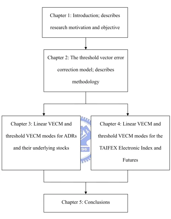
(17) estimation of the threshold parameters and tests for threshold effects. Chapter 3 applies linear VECM and threshold VECM models to the dynamic relationship between the prices of ADRs and their underlying stocks. Chapter 4 applies linear VECM and threshold VECM models to the effect of transaction cost reduction and the lead-lag relationship between the TAIFEX electronic index and futures. Brief conclusions, along with the summary drawn from this dissertation, are provided in Chapter 5.. 5.

(18) Chapter 1: Introduction; describes research motivation and objective. Chapter 2: The threshold vector error correction model; describes methodology. Chapter 3: Linear VECM and. Chapter 4: Linear VECM and. threshold VECM modes for ADRs. threshold VECM modes for the. and their underlying stocks. TAIFEX Electronic Index and Futures. Chapter 5: Conclusions. Figure 1. Research structure.. 6.

(19) 2. The Threshold Vector Error Correction Model A natural approach to modeling economic variables is defining different states of the world/regimes in order to determine the likelihood of a time-dependent economic variable occurring at a particular time. According to Aslanidis and Kouretas (2005), two main classes of regime-switching models have been proposed in the literature for modeling economic variables. The first class of models is the Tong and Lim (1980) initially proposed another approach which considers modeling explicitly the regime as a continuous function of an observable variable as in threshold autoregressive models. Although data have been gathered using this approach, statistical analysis techniques provide a better understanding of the regime. The second class of models is the Markov-switching type models, as originally employed in the business cycle context by Hamilton (1989). This approach assumes that the regime cannot actually be observed because the regime is determined by an underlying stochastic process. The threshold vector error correction model (VECM) has been the major model used to analyze the macroeconomic dynamic or the causal relationships of stock prices. Examples of the applications of VECM include articles by Agrawal (2001), Calza, Gartner, and Sousa (2003), and Chen and Lin (2004).. 2.1. Estimation of the Threshold Parameters Let ∆xt be a p-dimensional I (1) time series, with n observations, with l as the optimal lag length. A linear VECM of order l + 1 can be written briefly as: ∆xt = A' X t -1 ( β ) + u t. 7. (1).

(20) where X t −1 ( β ) = [1 wt −1 ( β ) ∆xt −1 ∆xt − 2 L ∆xt −l ] ' where ∆ is the first-order difference operator; the regressor X t −1 ( β ) is k × 1; A is k × p; and k = p l + 2. The error term u t is assumed to be a vector martingale difference sequence (MDS) with finite covariance matrix ∑ = E (u t u t ' ) . Note that wt-1 (β) = β ′xt −1 is an I (0) error correction term. Consider now an extension of equation (1), provided by: ⎧⎪A1 ' X t -1 ( β ) + u t , if wt −1 ( β ) ≤ γ , ∆x t = ⎨ ⎪⎩A 2 ' X t -1 ( β ) + u t , if wt −1 ( β ) > γ. (2). where γ is the threshold parameter. Note that this dissertation uses the absolute value of error correction term as a threshold variable. In addition to being parsimonious in the modeling of threshold effect, use of this term is reasonable since transaction costs tend to be symmetric both long-term and short-term for arbitrage. Alternatively, this may be written as: ∆x t = A1 ' X t -1 ( β )d1t ( β , γ ) + A 2 ' X t -1 ( β )d 2t ( β , γ ) + u t ,. where d 1t ( β , γ ) = 1( wt −1 ( β ) ≤ γ ), d 2t ( β , γ ) = 1( wt −1 ( β ) > γ ). and 1(．) denotes the indicator function. The existence of the threshold effect is confirmed if 0 < P ( wt −1 ( β ) ≤ γ ) < 1 ; otherwise the model simplifies to linear cointegration.. 8. (3).

(21) The threshold VECM can be estimated using the maximum likelihood method proposed by Hansen and Seo (2002). Under the assumption that the errors ut are iid Gaussian, the likelihood function is: n 1 n ′ Ln ( A1 , A2 , ∑, β , γ ) = − log Σ − ∑ ut ( A1 , A2 , β , γ ) ∑ −1ut ( A1 , A2 , β , γ ) , 2 t =1 2. (4). where ut ( A1 , A2 , β , γ ) = ∆xt − A1′ X t −1 ( β )d1t (β , γ ) − A2′ X t −1 ( β )d 2t (β , γ ) .. ˆ , βˆ , γˆ ) are the values that maximize L ( A , A , Σ, β , γ ) in order to maximize MLE ( Aˆ1 , Aˆ 2 , ∑ n 1 2. (. ). the log-likelihood, to hold ( β , γ ) fixed, and to compute the constrained MLE for Aˆ 1 , Aˆ 2 , ∑ˆ . This is just OLS regression: −1. ⎛ n ⎞ ⎛ n ⎞ Aˆ1 (β , γ ) = ⎜ ∑ X t −1 ( β ) X t −1 ( β ) ′ d 1t (β , γ )⎟ ⎜ ∑ X t −1 ( β ) ∆ x 't d 1t (β , γ )⎟ , ⎝ t =1 ⎠ ⎝ t =1 ⎠. (5). −1. ⎛ n ⎞ ⎛ n ⎞ Aˆ 2 (β , γ ) = ⎜ ∑ X t −1 ( β ) X t −1 ( β ) ′ d 2 t (β , γ )⎟ ⎜ ∑ X t −1 ( β ) ∆ x 't d 2 t (β , γ )⎟ , ⎝ t =1 ⎠ ⎝ t =1 ⎠. (. (6). ). uˆ t (β , γ ) = u t Aˆ1 (β , γ ), Aˆ 2 (β , γ ), β , γ ,. and n ′ ˆ (β , γ ) = 1 ∑ uˆ t (β , γ ) uˆ t (β , γ ) . ∑ n t =1. (7). Note that equations (4) and (5) are the OLS regressions of ∆xt on X t −1 ( β ) for the samples of wt −1 ( β ) ≤ γ and wt −1 ( β ) > γ , respectively.. (. ). ˆ (β , γ ), β , γ = − n log ∑ ˆ (β , γ ) − np . Ln (β , γ ) = Ln Aˆ1 (β , γ ), Aˆ 2 (β , γ ), ∑ 2 2. (8). From the grid search procedure, the model with the lowest value of log ∑ˆ (β , γ ) is used to provide the MLE ( βˆ , γˆ ) , while the limitation of β is π 0 ≤ P ( wt −1 ( β ) ≤ γ ) ≤ 1 − π 0 , where. 0 <π0 <1 is a trimming parameter. Andrews (1993) suggests setting π 0 between 0.05 and 0.15;. 9.

(22) this dissertation sets π 0 = 0.05. This dissertation employs the grid-search algorithm developed by Hansen and Seo (2002) to obtain the parameter estimates, with the MLE ( Aˆ 1 , Aˆ 2 ) being. ( ). ( ). ˆ =A ˆ βˆ , γˆ and Aˆ = Aˆ βˆ , γˆ . A 1 1 2 2. 2.2. Tests for Threshold Effects. Let H 0 represent the class of linear VECM in equation (1) and H 1 represent the class of tworegime threshold VECM in equation (2). These models are nested, with the '. '. constraint H 0 being the models in H 1 which gratify A1 = A2 . The test used here will compare H 0 (linear cointegration) with H 1 (threshold cointegration).. Hansen and Seo (2002) consider LM statistics for the threshold parameter. They do this for two reasons. First, the LM statistic is computationally quick, enabling feasible implementation of the bootstrap. Second, a likelihood ratio (LR) or Wald-type test would require a distribution theory for the parameter estimates for the unrestricted model, which they do not yet have. They now derive the LM test statistic. Assume for the moment that ( β , γ ) are known and fixed. The model under H 0 is equation (1), and the model under H 1 is equation (2). Given ( β , γ ) , the models are linear, so the MLE is least squares. As equation (1) is nested in equation (2) and the models are linear, an LM-like statistic with robust heteroskedasticity can be calculated from a linear regression on equation (2). The robust heteroskedasticity LM-like statistic is as follows:. (. )(. ). ′ −1 LM (γ ) = vec Aˆ1 (γ ) − Aˆ 2 (γ ) Vˆ1 (γ ) + Vˆ2 (γ ) × vec Aˆ (γ ) − Aˆ (γ ). (. 1. 2. where. 10. ). (9).

(23) Vˆ1 ( β , γ ) = M 1 ( β , γ ) −1 Ω1 ( β , γ ) M 1 ( β , γ ) −1 , Vˆ2 ( β , γ ) = M 2 ( β , γ ) −1 Ω 2 ( β , γ ) M 2 ( β , γ ) −1 , M 1 ( β , γ ) = I p ⊗ X 1 ( β , γ )′ X 1 ( β , γ ) , M 2 ( β , γ ) = I p ⊗ X 2 ( β , γ )′ X 2 ( β , γ ) , Ω1 ( β , γ ) = ξ1 ( β , γ )′ξ1 ( β , γ ) , Ω 2 ( β , γ ) = ξ 2 ( β , γ )′ξ 2 ( β , γ ) .. If β and γ were known, (9) would be the test statistic. When they are unknown, the LM ~ statistic is (9) evaluated at point estimates obtained under H 0 . The null estimate of β is β in Section 2.1, but there is no estimate of γ under H 0 , so there is no conventionally defined LM statistic. Davies (1987) proposes the statistic. ( ). ~ SupLM = sup LM β , γ rL ≤r ≤rU. (10). ~ , For this test, [rL , rU ] is the search region and is set so that rL is the π 0 percentile of w t −1 and rU is the (1 − π 0 ) percentile. Andrews (1993) argues that setting π 0 between 0.05 and 0.15 is typically a good choice. If the true cointegrating vector β 0 is known a priori, the test takes form (10), except that. β is fixed at the known value β 0 . Hansen and Seo (2002) denote this test statistic as. SupLM0 = sup LM (β0 , γ ) rL ≤r ≤rU. (11). Hansen and Seo (2002) believe that it is important to know that the values of γ that maximize the expressions in (10) and (11) will be different from the MLE γˆ presented in Section 2.1. Two separate reasons explain why these values are different. First, (10) and (11) were LM tests that were based on parameter estimates obtained under the null rather than the. 11.

(24) alternative. Second, the LM statistics were computed with heteroskedasticity-consistent covariance matrix estimates. For this case, even the maximum of the SupWald statistics were different from the MLE (the latter equal only when homoskedastic covariance matrix estimates are used). This difference is generic in threshold testing and estimation for regression models but not specific to threshold cointegration. Finally, this dissertation follows Hansen and Seo (2002) in developing two bootstrap methods to calculate critical values and P-values.. 12.

(25) 3. An Application to ADRs and Their Underlying Stocks 3.1. Literature Review Over the past decade, several researchers have examined the direct and indirect causal transmissions among American Depository Receipts (ADRs) and their underlying stocks (UNDs). Among others, Alaganar and Bhar (2001) have examined whether arbitrage opportunities exist between ADRs and their UNDs within the developed markets, while Rabinovitch, Silva, and Susmel (2003) have investigated this issue within the emerging markets. However, these studies generally found that the prices of both the ADRs and UNDs were the same, leaving little, if any, opportunities for arbitrage. Under perfect market assumptions, the ADRs and UNDs are closely related according to the law of one price. However, in practice, deviations from this no-arbitrage relation are usually observed because of market imperfections such as transaction costs and price uncertainty due to noise trader risk. Using the VECM, Kim, Szakmary, and Schwarz (2000) examined the dynamic price relationship of ADRs to exchange rates and UNDs. As arbitrage activities occur only when the spread between ADRs and UNDs is large enough to cover transaction costs, the use of threshold VECM could be potentially more meaningful in characterizing the price dynamics. Ely and Salehizadeh (2001) employed cointegration techniques and estimated error correction models to examine the degree of integration between the United States and three foreign equity markets: UK, Japan, and Germany. They found that ADRs were cointegrated with ordinary shares trading between the three foreign markets, which implied that for longterm investors, they are a substitute for ordinary shares. Their analysis of the dynamic. 13.

(26) relationships between ADRs and foreign equities suggested that information arising during trading hours from all the markets in the study affected portfolio valuation. Chen, Chou, and Yang (2002) examined the price transmission effect between ADRs/ global depository receipts (GDRs) and their respective UNDs. An error-correction model was used to analyze the long-run causal relations where the stock returns data was nonstationary. They also discussed the impact of premium and/or discount prices for overseas-listed stocks on the price transmission effect. Their results revealed a unidirectional causality from Taiwan’s capital market to other foreign markets. This asymmetry suggested that the domestic market plays a dominant role in price transmission relative to the foreign markets. Besides, both markets’ prices will adjust to establish a long-run cointegrated equilibrium. Wang and Lin (2005) investigated the price interaction and arbitrage opportunities provided by the dual listing between the ADRs and their foreign UNDs. To inspect the linkage between the Taiwanese ADRs and their underlying shares, they applied the threshold cointegration model, which allowed for asymmetric adjustment towards a long-run equilibrium. They also examined the short-term adjustments by employing the threshold error correction model. Since some evidence of asymmetric adjustments was found in the results of the data, they implemented a complete multivariate threshold cointegration model instead of the univariate model to test for these asymmetries and determine the maximum likelihood estimation. To the best of my knowledge, no study has yet been published characterizing the price dynamics between ADRs and UNDs through the use of the threshold VECM. Therefore, this dissertation explores two areas: the existence of arbitrage regimes and causal linkages. 14.

(27) between the prices of ADRs and UNDs. First of all, it identifies the location of possible thresholds and explores the relationship leading to the determination of the error correction term in a two-regime strategy. Second, it estimates a threshold cointegration framework in both the short-run and the long-run and finds that a significant threshold effect exists in the error correction term of the prices of ADRs and UNDs.. 3.2. Linear and Threshold Modes of VECM for ADR and Its UND For ADR and UND, transaction costs and other market imperfection factors might cause the error correction effects on the price adjustment to be significant only when the deviation of price between ADR and UND is larger than a certain threshold. While previous studies, such as that of Enders and Chumrusphonlert (2004), employed a univariate threshold model to explore the properties of purchasing power parity, this research follows Hansen and Seo’s (2002) model to develop a multivariate threshold VECM. The model is employed to estimate the threshold parameters, to construct confidence intervals for the threshold parameters, and to develop new tests for the threshold effects of ADR and UND prices. 3.2.1. Estimation of the Threshold Parameters. This research applied the linear and the threshold VECM model to ADR and UND. Let ∆xt be a p-dimensional I (1) time series, with n observations, with l as the optimal lag length. A linear VECM (12) of order l + 1 can be written briefly as:. 15.

(28) p. p. i =1. i =1. ∆UNDt = α10 + α11 wt -1 ( β ) + ∑ β1i ∆ADRt −i + ∑ β 2i ∆UNDt −i + u 1t , p. p. j =1. j =1. ∆ADRt = α 20 + α 21wt -1 ( β ) + ∑ β1 j ∆ADRt − j + ∑ β 2 j ∆UNDt − j + u 2t. (12). where ∆ is the first-order difference operator. The error term ut is assumed to be a vector martingale difference sequence with finite covariance matrix ∑ = E (u t u t ' ) . Note that. wt-1 (β) = β ′xt −1 is an I (0) error correction term. The linear VECM model explains the price changes for short-term as well as long-term adjustment (Figure 2). If the deviation from the long-term equilibrium is greater than the threshold γ, the price transmission process is defined by a different regime (regime 2) than in the case of smaller deviations from the long-term equilibrium (regime 1). As a variant and in line with approaches by Balke and Fomby (1997), the following specification of a threshold VECM (13) is proposed: Regime 1 p. p. i =1. i =1. ∆UNDt = α10 + α11 wt -1 ( β ) + ∑ β1i ∆ADRt −i + ∑ β 2i ∆UNDt −i + u1t , p. p. j =1. j =1. ∆ADRt = α 20 + α 21 wt -1 ( β ) + ∑ β1 j ∆ADRt − j + ∑ β 2 j ∆UNDt − j + u 2t ,. if wt −1 ( β ) ≤ r , if wt −1 ( β ) ≤ r ,. Regime 2 p. p. i =1. i =1. p. p. j =1. j =1. ∆UNDt = α 30 + α 31 wt -1 ( β ) + ∑ β1i ∆ADRt −i + ∑ β 2i ∆UNDt −i + u1t , ∆ADRt = α 40 + α 41 wt -1 ( β ) + ∑ β1 j ∆ADRt − j + ∑ β 2 j ∆UNDt − j + u 2t ,. if wt −1 ( β ) > r , if wt −1 ( β ) > r (13). where γ is the threshold parameter. Note that this research uses the absolute value of error correction term as a threshold variable, as explained earlier.. 16.

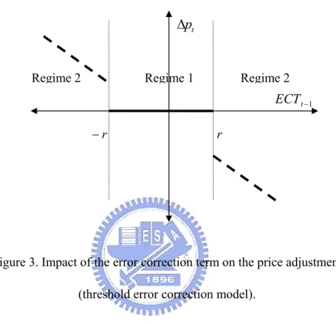
(29) ∆pt. ECTt −1. Figure 2. Impact of the error correction term on the price adjustment (linear error correction model).. This specification excludes the possibility of smaller deviations from a long-term equilibrium inside a regime of adjustment to larger deviations (Figure 3). Specification (13) allows this and is therefore economically more meaningful. Using threshold VECM (13), two regimes of price adjustment are used: one defined by absolute deviations from the long-term equilibrium that are below the threshold r (regime 1) and another defined by deviations that exceed the threshold r in absolute values (regime 2). Because of this regime definition, the threshold VECM is based on only one threshold and therefore is testable regarding threshold significance but also potentially allows for the economically meaningful regime 1 inside a regime of price adjustment to greater deviations from the long-term equilibrium (regime 2). Note that threshold VECM (13) is essentially a restricted version of the general two-threshold model depicted; this is restricted in the sense that no asymmetric price transmission is. 17.

(30) possible in (13), as the same price reaction occurs regardless of whether ECTt-1 is larger than γ or smaller than − r .. ∆pt. Regime 2. Regime 1. Regime 2. ECT t −1 −r. r. Figure 3. Impact of the error correction term on the price adjustment (threshold error correction model).. The threshold VECM of ADR and UND can be estimated using the maximum likelihood method proposed by Hansen and Seo (2002). 3.2.2. Tests for Threshold Effects. In order to assess the evidence, both the linear and the threshold VECM were tested by using the Lagrange Multiplier test developed by Hansen and Seo (2002). The test is used when the true cointegrating vector is unknown a priori and is denoted as:. ( ). ~ SupLM = sup LM β , γ rL ≤r ≤rU. 18. (14).

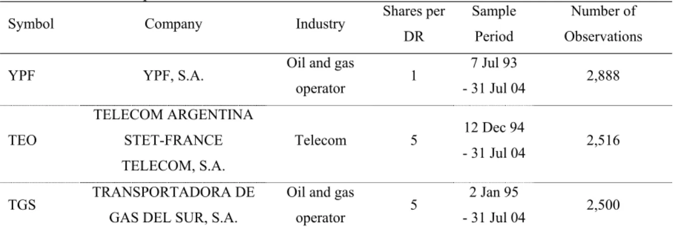
(31) ~ where β is the null estimate of β . For this test, [rL , rU ] is the search region set so that rL is ~ , and r is the (1 − π ) percentile; this study sets π = 0.05. Finally, the π 0 percentile of w t −1 U 0 0 Hansen and Seo (2002) developed two bootstrap methods to calculate critical values and Pvalues.. 3.3. Data and Empirical Results The ADR and UND series were tested for stationarity in this study using unit root tests; followed by an examination of the cointegration test between the two series. If they were cointegrated, the threshold VECM was then applied to determine the short-run dynamics and the long-run equilibrium between the ADR and the UND markets. The daily returns of three locally traded Argentinean firms provided the data for analysis in this study, with Table 1 providing the basic description of their respective New York Stock Exchange-traded ADRs. Although the ADRs are priced in US dollars, UNDs in the home stock market are priced in Argentinian pesos. The prices of ADRs are calculated into the Argentinian peso price using the daily closing exchange rate. ADRs prices, the prices of UNDs, and the exchange rates used in this study were obtained from Datastream. Table 1. Data description Symbol. Company. YPF. YPF, S.A.. Industry Oil and gas operator. Shares per. Sample. Number of. DR. Period. Observations. 1. TELECOM ARGENTINA TEO. STET-FRANCE. Telecom. 5. TELECOM, S.A. TGS. TRANSPORTADORA DE. Oil and gas. GAS DEL SUR, S.A.. operator. 19. 5. 7 Jul 93 - 31 Jul 04 12 Dec 94 - 31 Jul 04 2 Jan 95 - 31 Jul 04. 2,888. 2,516. 2,500.

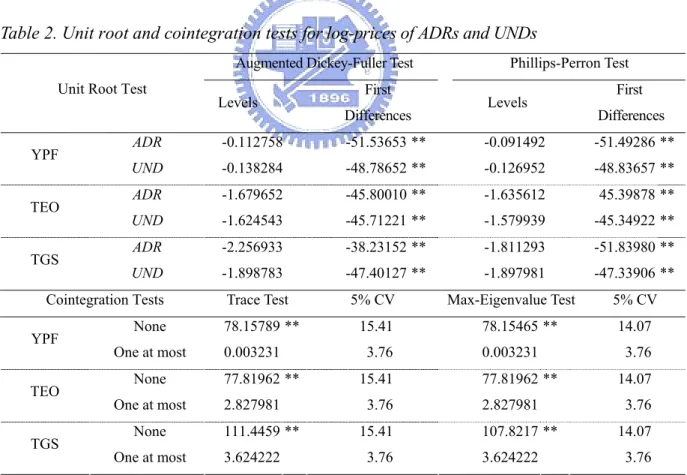
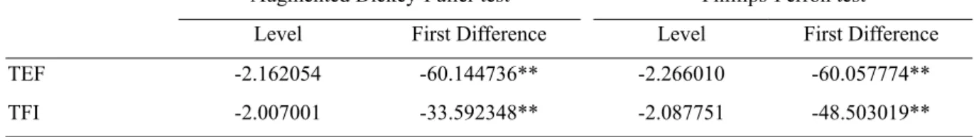
(32) The log-price of the ADRs and the UNDs was used to carry out this empirical analysis, with the returns of ADRs and UNDs being calculated, first of all, by taking the difference in the log-price. Table 2 presents the results of the unit root and cointegration tests; the unit root test used the null hypothesis versus the alternative of stationarity in the variables for the results of the Augmented Dickey-Fuller (ADF) and Phillips-Perron (PP) tests. The results thus cannot reject the null hypothesis of a unit root; the variables in the levels were I (1) for each ADR price and UND price. The variables in the first difference were integrated of order zero; the null hypothesis of unit root was rejected at the 5% level for the price difference series. These results indicate that the two price series are integrated in the first difference and thus validate the use of the cointegration test. Table 2. Unit root and cointegration tests for log-prices of ADRs and UNDs Augmented Dickey-Fuller Test Unit Root Test. YPF TEO TGS. TEO TGS. First Differences. Levels. First Differences. ADR. -0.112758. -51.53653 **. -0.091492. -51.49286 **. UND. -0.138284. -48.78652 **. -0.126952. -48.83657 **. ADR. -1.679652. -45.80010 **. -1.635612. 45.39878 **. UND. -1.624543. -45.71221 **. -1.579939. -45.34922 **. ADR. -2.256933. -38.23152 **. -1.811293. -51.83980 **. UND. -1.898783. -47.40127 **. -1.897981. -47.33906 **. Max-Eigenvalue Test. 5% CV. Cointegration Tests YPF. Levels. Phillips-Perron Test. None One at most None One at most None One at most. Trace Test. 5% CV. 78.15789 **. 15.41. 0.003231. 3.76. 77.81962 **. 15.41. 2.827981. 3.76. 111.4459 **. 15.41. 3.624222. 3.76. 78.15465 ** 0.003231 77.81962 ** 2.827981 107.8217 ** 3.624222. 14.07 3.76 14.07 3.76 14.07 3.76. Notes: 1 Total number of sample observations is 2,888 for YPF, 2,516 for TEO, and 2,500 for TGS. UND represents price of underlying stock. ** P < 0.05.. 20.

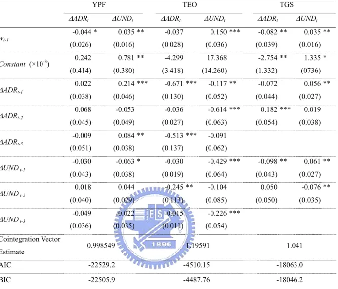
(33) Given that all the variables of the same order were integrated, this study used two Johansen multivariate cointegration tests to determine whether the variables in each series were cointegrated. The maximum likelihood estimation procedure provided a likelihood ratio test, referred to as a trace test, with the likelihood ratio test being the test for maximum eigenvalue. The likelihood ratio statistic rejected the null hypothesis of no cointegration at the 5% level. A feature of this approach is that the VECM contains an error correction term that reflects the current error in achieving long-run equilibrium. Therefore, the VECM can be used to jointly estimate the long-run relationship with short-run dynamics, a process that has been proven to be more effective than Granger causality. Table 3 provides the estimates of the linear model. To address the issue of linear, or nonlinear, adjustment to the long-run equilibrium, this study estimated a linear VECM, given by equation (11), with the selection of the lag length being based upon the AIC and BIC criteria. As a comparison, this study first of all estimated the linear VECM for the price series of the ADRs and UNDs, reporting the results of the linear VECM estimation in Table 3. The estimated coefficients of the error correction term on the equations of the UND were all significant at the 5% level.. 21.

(34) Table 3. Linear VECM estimations for log-prices of ADRs and UNDs YPF. ∆ADRt. TEO. ∆UNDt. -0.044 *. wt-1. (0.026). Constant (×10-3). ∆ADRt-1 ∆ADRt-2 ∆ADRt-3 ∆UND t-1 ∆UND t-2 ∆UND t-3 Cointegration Vector. 0.035 ** (0.016). 0.242 (0.414). 0.781 ** (0.380). 0.022. 0.214 ***. ∆ADRt. ∆UNDt. -0.037. (0.036). -4.299. 17.368. (3.418). (14.260). -0.671 ***. (0.046). (0.130). 0.068. -0.053. -0.036. (0.045). (0.049). (0.027). (0.051). 0.084 ** (0.038). -0.030. -0.063 *. 0.150 ***. (0.028). (0.038). -0.009. TGS. (0.052) -0.614 *** (0.063). -0.513 *** (0.137). (0.038). 0.018. 0.044. (0.040). (0.029). (0.113). -0.049. -0.022. -0.015. (0.036). (0.035). (0.011). ∆UNDt. -0.082 ** (0.039). 0.035 ** (0.016). -2.754 ** (1.332). 1.335 * (0736). -0.072. 0.056 **. (0.044). (0.027). 0.182 *** (0.054). 0.019 (0.038). -0.091 (0.062). -0.030. (0.043). -0.117 **. ∆ADRt. -0.429 ***. (0.019) -0.245 **. -0.098 **. (0.064). (0.043). -0.104. 0.050. (0.085). (0.050). 0.061 ** (0.027) -0.076 ** (0.035). -0.226 *** (0.054). 0.998549. 1.19591. 1.041. AIC. -22529.2. -4510.15. -18063.0. BIC. -22505.9. -4487.76. -18046.2. Estimate. Notes: 1 Values in parentheses are Eicker-White standard errors. ***P < 0.01; **P < 0.05; * P < 0.10.. The estimation results of the threshold VECM, and the test for the hypothesis of linearity versus the threshold effect of nonlinearity, provided by equation (13), are presented in Tables 4, 5 and 6, under the application of the SupLM test for the complete bivariate specification. The P values of the results supporting the threshold cointegration hypothesis were calculated using both the fixed repressor and a residual bootstrap experiment, with 1,000 simulation replications. The estimated threshold VECM was provided by equation (12), with the selection of the lag length being based upon the AIC and BIC criteria; it was also considered. 22.

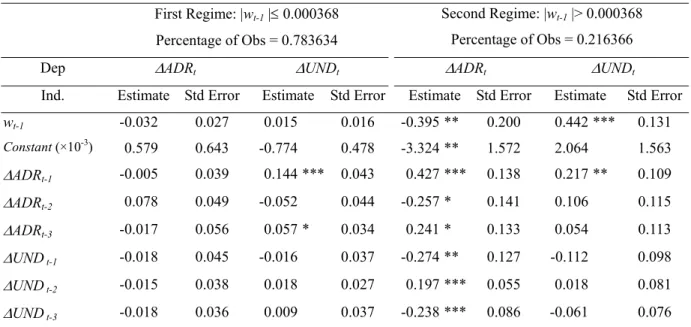
(35) in this study that the cointegrating vector βˆ should be estimated. Standard errors were calculated from the heteroskedasticity-robust covariance estimator, with the parameter estimates being calculated by the minimization of equation (8) over a 300 × 300 grid on the parameters ( β , γ ). Table 4 reports the threshold VECM results for ADR with ticker symbol ‘YPF’ along with UND. In this study, a lag length of l = 3 was selected, with the estimated cointegrating relationship being wt-1 = ADRt-1 −1.00123UNDt-1, quite close to a unit coefficient. This study also conducted analyses for the case where a unit coefficient is imposed, with the results being very similar. The estimated threshold parameter was γ = 0.000368, indicating that the first regime corresponded to |ADRt-1 −1.00123UNDt-1| ≤ 0.000368. This first regime, which comprised 78% of all of the observations in the sample, is referred to in this study as the ‘typical’ regime. Conversely, the second regime, which was |ADRt-1 −1.00123UNDt-1| > 0.000368, comprised 22% of all of the observations in the sample and is referred to here as the ‘extreme’ regime. In the ‘typical’ regime specifically, both ∆ADRt and ∆UNDt had statistically insignificant error correction effects and minimal dynamics. They were close to white noise, which indicates that in this regime, ADRt and UNDt were close to random walks. In contrast, in the ‘extreme’ regime, the asymmetry of ∆ADRt and ∆UNDt was implied, in the sense that there was an error correction effect in the ADR and UND equation being statistically significant with dynamic coefficients. All in all, ADRt and UNDt were statistically significant in the error correction effects in the ‘extreme’ regime, but not in the ‘typical’ regime.. 23.

(36) Table 4. Threshold VECM estimations of YPF for log-prices of ADR and UND First Regime: |wt-1 |≤ 0.000368. Second Regime: |wt-1 |> 0.000368. Percentage of Obs = 0.783634. Percentage of Obs = 0.216366. Dep. ∆ADRt. Ind.. Estimate Std Error. Estimate. -0.032. 0.027. 0.015. 0.016. -0.395 **. 0.200. 0.442 ***. 0.131. 0.579. 0.643. -0.774. 0.478. -3.324 **. 1.572. 2.064. 1.563. ∆ADRt-1. -0.005. 0.039. 0.138. 0.217 **. 0.109. ∆ADRt-2. 0.078. 0.049. ∆ADRt-3. -0.017. 0.056. ∆UND t-1. -0.018. 0.045. ∆UND t-2. -0.015. ∆UND t-3. -0.018. wt-1 -3. Constant (×10 ). ∆UNDt. 0.144 *** -0.052. ∆ADRt. Std Error. 0.043. Estimate. 0.427 ***. ∆UNDt. Std Error. Estimate. Std Error. 0.044. -0.257 *. 0.141. 0.106. 0.115. 0.034. 0.241 *. 0.133. 0.054. 0.113. -0.016. 0.037. -0.274 **. 0.127. -0.112. 0.098. 0.038. 0.018. 0.027. 0.197 ***. 0.055. 0.018. 0.081. 0.036. 0.009. 0.037. -0.238 ***. 0.086. -0.061. 0.076. 0.057 *. Threshold Estimate = 0.000368; Cointegrating Vector Estimate = 1.00123; AIC= -22653.1; BIC = -22606.4 Lagrange Multiplier Threshold Test Fixed Regressor bootstrap = 84.114*** (P < 0.001) Residual bootstrap = 28.306*** (P < 0.001 ) Wald Test Equality of Dynamic Coefficients = 34.188*** (P < 0.001) Equality of EC Coefficients = 24.911*** (P = 0.008) Note: ***P < 0.01; **P < 0.05; *P < 0.10.. The evidence of nonlinearity appeared to gain strength from the results of the Wald test diagnostics; thus, the null hypothesis of linearity in error correction terms was rejected. Comparing the estimated coefficients of the error correction terms in Tables 3 and 4 shows that the linear error correction models imply very slow speed of adjustment, a result consistent with that reported in Enders and Chumrusphonlert (2004). Since the null hypothesis is of equality of the coefficients on the error correction terms and of the dynamic coefficients across the two regimes, an important finding of the estimated linear VECM and threshold VECM is that the error correction term for the ADR was negative; this result is consistent with the error correction terms. This implies specifically that from the long-run equilibrium, the ADR adjusts to any short-run deviations. Furthermore, the negative sign of the error. 24.

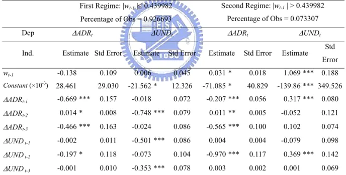
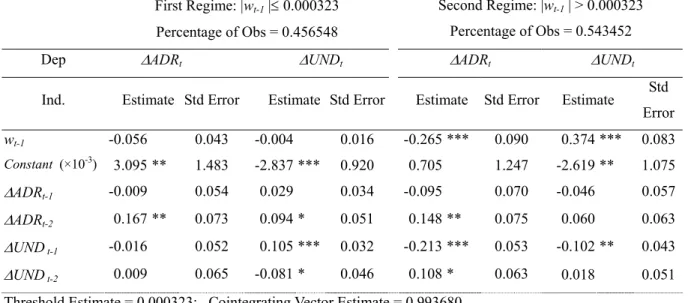
(37) correction term implies that if the ADR premium is above its equilibrium level, the ADR will decline. This was as predicted in the model when the ADR overshot its long-run equilibrium; the result is therefore just as expected. Details of the procedures and analyses provided above are also presented in Tables 5 and 6. The error correction term appeared to be significant only in the ‘extreme’ regime. The estimated coefficients of the error correction terms in the ‘extreme’ regime appeared to be larger than those in the linear VECM. The short-run dynamic effects of ADRs and UNDs showed significant differences between ‘typical’ and ‘extreme’ regimes.. Table 5. Threshold VECM estimations of TEO for log-prices of ADR and UND First Regime: |wt-1 |≤ 0.439982. Second Regime: |wt-1 | > 0.439982. Percentage of Obs = 0.926693. Percentage of Obs = 0.073307. ∆ADRt. Dep Ind.. ∆UNDt. Estimate Std Error. wt-1. Estimate. ∆ADRt. ∆UNDt. Std Error. Estimate. Std Error. Estimate. Std Error. -0.138. 0.109. 0.006. 0.045. 0.031 *. 0.018. 1.069 *** 0.188. Constant (×10 ). 28.461. 29.030. -21.562 *. 12.326. -71.085 *. 40.829. -139.86 *** 349.526. ∆ADRt-1. -0.669 ***. 0.157. -0.018. 0.072. -0.207 ***. 0.056. 0.317 *** 0.080. 0.008. -0.748 ***. 0.079. 0.011 **. 0.005. -0.052. 0.121. -0.565 ***. 0.100. 0.102. 0.074. 0.004. -0.079. 0.098. -3. ∆ADRt-2. 0.014 *. ∆ADRt-3. -0.466 ***. 0.163. -0.024. 0.086. ∆UND t-1. -0.002. 0.011. -0.501 ***. 0.086. ∆UND t-2. -0.197 *. 0.118. -0.073. 0.104. ∆UND t-3. -0.001. 0.010. -0.353 ***. 0.078. 0.004 -0.970 *** 0.003. 0.117. 0.369 *** 0.142. 0.002. 0.001. 0.069. Threshold Estimate = 0.439982; Cointegrating Vector Estimate = 0.789472; AIC = -4740.20; BIC= -4695.41 Lagrange Multiplier Threshold Test Fixed Regressor bootstrap = 103.117*** (P < 0.001) Residual bootstrap = 34.232*** (P < 0.001 ) Wald Test Equality of Dynamic Coefficients = 24.806*** (P < 0.001) Equality of EC Coefficients = 26.127*** (P < 0.001) Note: ***P < 0.01; **P < 0.05; *P < 0.10.. 25.

(38) Table 6. Threshold VECM estimations of TGS for log-prices of ADR and UND First Regime: |wt-1 |≤ 0.000323. Second Regime: |wt-1 | > 0.000323. Percentage of Obs = 0.456548. Percentage of Obs = 0.543452. ∆ADRt. Dep Ind.. Estimate Std Error. wt-1. -0.056 -3. Constant (×10 ). ∆ADRt-1 ∆ADRt-2. ∆UNDt. 3.095 ** -0.009 0.167 **. Estimate Std Error. ∆ADRt Estimate -0.265 ***. ∆UNDt. Std Error. Estimate. 0.090. 0.374 ***. Std Error. 0.043. -0.004. 0.016. 1.483. -2.837 ***. 0.920. 0.705. 1.247. -2.619 **. 1.075. -0.095. 0.070. -0.046. 0.057. 0.060. 0.063. 0.054. 0.029. 0.034. 0.073. 0.094 *. 0.051. 0.148 **. 0.075. 0.105 ***. 0.032. -0.213 ***. 0.053. ∆UND t-1. -0.016. 0.052. ∆UND t-2. 0.009. 0.065. -0.081 *. 0.046. 0.108 *. 0.063. -0.102 ** 0.018. 0.083. 0.043 0.051. Threshold Estimate = 0.000323; Cointegrating Vector Estimate = 0.993680 AIC = -18146. 3; BIC = -18112.8 Lagrange Multiplier Threshold Test Fixed Regressor bootstrap = 20.910*** (P < 0.001) Residual bootstrap = 17.305*** (P < 0.001 ) Wald Test Equality of Dynamic Coefficients = 20.772*** (P = 0.008) Equality of EC Coefficients = 49.256*** (P < 0.001) Note: ***P < 0.01; **P < 0.05; *P < 0.10.. 3.4. Summary This study employed the threshold VECM to investigate the dynamic price relationship between ADRs and their UNDs. The results provided by the LM test statistics rejected the null hypothesis of no threshold effect, while the Wald test results rejected the null hypothesis of the coefficients of the error correction term in the two regimes having the same value. This study therefore provides strong evidence to show that a threshold effect does exist in the prices of ADRs and their UNDs. The main findings of these analyses can be summarized as follows. First of all, the results based on the threshold VECM demonstrated that linearity is rejected in favor of threshold. 26.

(39) effect nonlinearity and that the estimated two-regime threshold VECM forms a statistically sufficient representation of the data with separating regimes. Secondly, through the threshold parameters, this study classified the ‘typical’ regime and the ‘extreme’ regime, with only the error correction effect appearing in the ‘extreme’ regime being statistically significant. Finally, the negative sign of the error correction term in the ‘extreme’ regime implies that if the ADR’s premium is above its equilibrium level, then the ADR price will decline; that is, nonlinear mean-reversion is evident. Last but not least, this study pointed to threshold VECM, which is consistent with the stylized fact of the error correction term, and suggested that the effectiveness of the threshold cointegration model surpasses that of the linear cointegration model. Further analytical studies using the threshold VECM model should be undertaken in the future, with its application being targeted at predicting the achievements of ADRs and UNDs.. 27.

(40) 4. Transaction Cost Reductions and the Lead-Lag Relationship Between the TAIFEX Electronic Index and Futures 4.1. Literature Review In 1982, the Kansas City Board of Trade (KCBT) in the U.S. introduced the first stock index futures in the world, the Value Line Composite Index. At the same time, the Chicago Mercantile Exchange (CME) introduced the Standard & Poor’s (S&P) 500 Stock Index, while the New York Stock Exchange (NYSE) introduced the NYSE Composite Stock Index. Since then, the stock index futures have grown rapidly and are now traded in many countries in the world. The most famous ones include the Financial Times Stock Exchange (FTSE) 100 stock index, introduced in 1984 by the London International Financial Futures and Options Exchange (LIFFE), and the Nikkei 225 stock index, created by the Osaka Securities Exchange (OSE) in 1989. Afterwards, Singapore began offering a Morgan Stanley Capital International (MSCI) Taiwan futures contract, the Taiwan Morgan Stanley Capital weighted stock index (TiMSCI) traded in Taiwan on the Singapore Exchange Derivatives Trading Limited (SGX-DT). The contract was introduced on January 9, 1997, when the Taiwan Stock Exchange (TSE) began attracting more foreign interest. However, on July 21, 1998, Taiwan introduced its own index futures contract to be traded on the Taiwan Futures Exchange (TAIFEX), which was called TAIFEX futures. In order to meet a strong market demand, TAIFEX began operating two stock indexes, the Electronic Sector Index Futures and the Finance Sector Index Futures, on July 21, 1999.. 28.

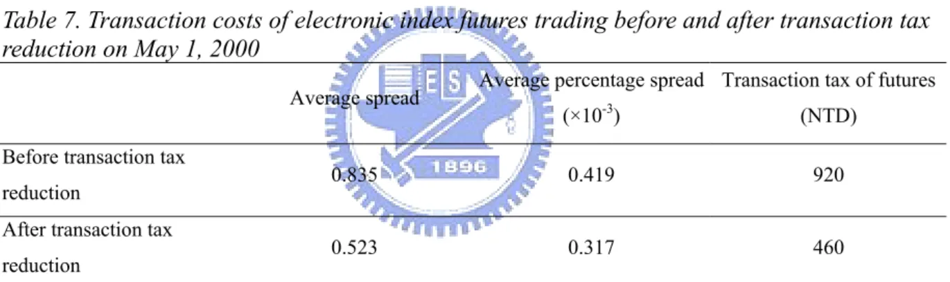
(41) To provide an attractive environment for investors, transaction costs should be low, assets should be liquid, and the competitive market should be efficient, meaning that information should be quickly and accurately reflected in prices. A fully competitive market can be achieved by immediately reducing information shock and lowering the costs of trading. Such a market would decrease price uncertainty and attract more investors into the market. In the development of the Taiwan futures, the government taxed the transactions, resulting in higher transaction costs. Corporations were unwilling to participate and the public was unfamiliar with this new market, resulting in lower trading volume. However, futures trading volume significantly increased when TAIFEX reduced the transaction tax from 5 basis points to 2.5 basis points in May 2000. Empirical tests were performed to examine the information transmission between prices of the TAIFEX Electronic Sector Index (TEI) and the TAIFEX Electronic Sector Index futures (TEF) for the sample periods before and after the tax reduction. According to the TAIFEX data, the TEF average trading volume per month was 17,045 from January to April 2000 and increased to 27,275 from May to August 2000, after the tax reduction. Thus, trading volume increased 1.6 times per month after the decrease. To my knowledge, no study has yet been published to characterize the TAIFEX electronic index and futures market stemming from a transaction tax reduction and the leadlag relationship by using the threshold vector error correction model (VECM). This study explores both pre- and post-tax reduction adjustment, the causal relationship between prices of the TEF and the TEI through the linear and threshold VECM models. An out-of-sample comparison was also conducted to determine the forecasting performance of the linear and. 29.

(42) threshold VECM. Obviously, transaction costs prevent arbitrageurs from realizing many valuable opportunities, as the mean-reversion will occur only when the deviation is large. In recent times, there has been extensive research related to transaction costs. Chou and Lee (2002) analyzed the differences in transaction costs and information transmissions between the SGX and the TAIFEX for the sample periods before and after tax reduction. They showed that the transaction cost reduction greatly increased the efficiencies of price execution. Hau (2005) discussed the causal linkage between transaction costs and financial volatility using two methodological improvements over prior research. He concluded that the effect of transaction costs on volatility is positive and significant, both statistically and economically. Baltagi, Li, and Li (2005) examined the impact on market behavior from a stamp-tax rate increase and found that trading volume decreased by one third when the tax rate increased by two thirds, while the markets’ volatility significantly increased. Furthermore, markets became less efficient due to the change in the volatility structure, meaning that shocks were slowly assimilated in the markets. According to the trading cost hypothesis of Fleming, Ostdiek, and Whaley (1996) and Kim, Szakmary, and Schwarz (1999), the market with the lowest transaction costs will react to new information the most quickly. Thus, we can determine that the market with the lowest transaction costs will tend to lead its competing markets. The studies fully support the trading cost hypothesis. Fleming, Ostdiek, and Whaley (1996) explored the S&P 500 futures, the S&P 100 options, and the underlying stock index portfolio’s intraday data to examine the temporal relationship. They found that, from the standpoint of the transaction cost hypothesis, when. 30.

(43) new information becomes available in a derivative financial market, the initial response should be more heavily reflected in the derivative price before the price of the underlying stock itself changes. It is shown that the S&P 500 futures lead the S&P options and the S&P 100 leads the underlying stocks of the S&P 100 index portfolio. These results support the trading cost hypothesis. Kim, Szakmary, and Schwarz’s (1999) study was conducted for the S&P 500, the NYSE, and the relationship between the Major Market Index (MMI) and stock market. They showed that the MMI leads the S&P 500 and the NYSE markets because the MMI has a better forecasting ability due to lower transaction costs than both the S&P 500 and the NYSE. However, the S&P 500 leads the other two markets in the stock market. All in all, the transaction cost hypothesis of price leadership and the trading cost hypothesis of price leadership are linked together. Once again, this transaction cost hypothesis is further supported. If the respective markets are free of impurities and reflect an efficient flow of information, then the returns on a spot market index and the associated futures contract should be perfectly correlated and consistent over time. In other words, the prices of the stock index and the futures price should simultaneously reflect new information as it becomes available. The theoretical relationship between a stock index futures price and its underlying asset, as indicated above, is known as the cost of carry model. However, several inefficiencies create a lead-lag relationship in stock index futures. Many researchers have studied the lead-lag relationship in the futures and stock markets. Some of those include Shyy, Vijayraghavan, and Scott-Quinn (1996); Abhyankar (1998); Chu,. 31.

(44) Hsieh, and Tse (1999); Min and Najand (1999); Turkington and Walsh (1999); Tse (1999); Frino, Walter, and West (2000); Chiang and Fong (2001); Kurov and Lasser (2002); Roope and Zurbruegg (2002); Chng (2004); Covrid, Ding, and Low (2004); and So and Tse (2004). Most of these researchers believe there is a price discovery function in the futures market. Using cointegration analysis and an error correction model, Roope and Zurbruegg (2002) showed both the Hasbrouck and Gonzalo-Granger methodologies for extracting the information content held in each market. Information efficiencies were compared between the Singapore Exchange and the Taiwan Futures Exchange for the Taiwan Index Futures listed in both markets. They found a dynamic flow of information and a price discovery between these exchanges, showing that futures prices considerably interact with each market. Although it is likely that Singapore prices will reflect new information first, they show that both futures markets now play a key role in price discovery. So and Tse (2004) studied the price discovery process among the Hong Kong Hang Seng Index markets. The price series of the index, futures, and tracker fund were cointegrated with one common factor. Their results argue that the futures market is the main driving force in the price discovery process, followed by the index, while the contribution of the tracker fund is unimportant. These findings are consistent with the well-documented observation that the futures market dominates the spot market in the price discovery process. Other research has been conducted about forecasting models, including publications by Brooks, Rew, and Ritson (2001), Clements and Galvão (2004), and Bradley and Jansen (2004), who compare the forecasting performance of the linear and nonlinear model. Using a number of time-series models, Brooks, Rew, and Ritson (2001) analyzed the lead-lag relationship. 32.

(45) between the FTSE 100 index and index futures price. They found that lagged changes in the futures price can help predict changes in the spot price. Clements and Galvão (2004) discussed whether there were nonlinearities in the response of short- and long-term interest rates to the spread and assessed the out-of-sample predictability of interest rates using linear and nonlinear models. They found strong evidence of nonlinearities in the response of interest rates to the spread. Bradley and Jansen (2004) modeled stock returns and industrial production as state-dependent and nonlinear; the dynamics depended on the sign and magnitude of past realized returns and the growth of industrial production. For stock returns, they found that the linear model generally did as well as, or better than, any of their nonlinear models. With growth in industrial production, two of their nonlinear models outperformed the linear model. Clements, Franses, and Swanson (2004) explored state-of-the-art estimations, evaluations, and selections among nonlinear forecasting models. They argue that although the evidence in favor of constructing a forecast using nonlinear models is rather sparse; there is a reason to be optimistic. De Gooijer and Vidiella-i-Anguera (2004) investigated that the longterm (one to sixty steps ahead) forecasting performance can further be enhanced by applying a nonlinear equilibrium correction model. Chung, Ho, and Wei (2005) followed Hansen and Seo’s (2002) model to develop a multivariate threshold VECM. Their study provided strong evidence to show that a threshold effect does exist in the prices of ADRs and their underlying stocks. Seo (2003) implies that information on the future change in the short-term interest rate can be determined by the yield curve from expectations hypothesis. However, transaction. 33.

(46) costs exist in the financial market, which prevent investors from taking advantage of the arbitrage opportunity because the arbitrage doesn’t always fully cover the transaction costs. This research used the threshold VECM, which allows for the nonlinear adjustment to the long-run equilibrium relationship, to assess the effect of transaction costs on the predictability of the term structure. Seo (2003) found a significant amount of threshold effect and determined that the adjustment coefficients were regime-dependent. The empirical results support the nonlinear mean reversion in the term structure of interest rates. The existence of the transaction tax is likely to affect the market quality of futures trading in a number of ways. Fleming, Ostdiek, and Whaley (1996) argue that three important components of trading costs are the bid-ask spread, brokerage commission, and market impact costs, in the form of price concessions for large trades. Another obvious trading expense is the transaction tax, which is a significant component in the TAIFEX and is addressed in this chapter of the dissertation. Kim, Szakmary, and Schwarz (1999) investigated the transaction cost hypothesis of price leadership to forecast whether lower transaction costs could rapidly respond to new information through vector autoregression for indices futures contracts. This dissertation addresses whether there is a nonlinear correlation between the TEF and the TEI; that is, if there are different price correlations between the TEF and the TEI under different circumstances. Further, different long-term equilibrium relations and short-term adjustments exist under different regimes.. 34.

(47) 4.2. Linear and Threshold Modes of the VCEM for the TAIFEX Electronic Index and Futures For the case prices of the TEF and the TEI, the existence of transaction costs and other market imperfections might cause the error correction effects on the price adjustment to be significant only when the deviation between prices of the TEF and the TEI is larger than a certain threshold. Threshold tests have been used in a variety of situations. Abdulai (2002) employed threshold cointegration tests that allowed for asymmetric adjustments towards a long-run equilibrium to examine the relationship of Switzerland’s pork prices between producers and retailers. The short-run adjustments were also examined with asymmetric error correction models and compared with the conventional symmetric error correction models. Arestis, Cipollini, and Fattouh (2004) contributed to the debate on whether the U.S.’s large federal budget deficits are sustainable in the long run; they used U.S. government deficit per capita as a threshold autoregressive process. Bajo-Rubio, Díaz-Roldán, and Esteve (2004) used the threshold autoregressive model through the evolution of the Spanish budget deficit to derive endogenously threshold effects. This type of study shows that once the threshold is reached, a mean-reverting dynamic behavior of the budget deficit should be expected. Tkacz (2004) used interest rate yield spreads to explain changes in inflation. That paper investigated whether such relationships can be modeled using two-regime threshold models. Here, Hansen and Seo’s (2002) model was used to develop a multivariate threshold VECM. The model was employed to estimate the threshold parameters, to construct. 35.

(48) confidence intervals for the threshold parameters, and to develop new tests for the threshold effect prices of the TEF and the TEI. 4.2.1. Estimation of the Threshold Parameters. This study used the linear and the threshold VECM model on TEF and TEI. Let ∆xt be a pdimensional I (1) time series, with n observations, with l as the optimal lag length. A linear VECM (15) of order l + 1 can be written briefly as: p. p. i =1. i =1. ∆TEI t = α10 + α11 wt -1 + ∑ β1i ∆TEFt −i + ∑ β 2i ∆TEI t −i + u1t , p. p. j =1. j =1. ∆TEFt = α 20 + α 21 wt -1 + ∑ β1 j ∆TEFt − j + ∑ β 2 j ∆TEI t − j + u 2t. (15). where ∆ is the first-order difference operator. The error term u t is assumed to be a vector martingale difference sequence with finite covariance matrix ∑ = E (u t u t ' ) . Note that. wt-1 = TEFt −1 −TEIt −1 is an I (0) error correction term. As a variant and in line with approaches by Balke and Fomby (1997), the following specification of a threshold VECM (16) is proposed: p p ⎡ ⎤ ∆TFI t = ⎢α10 + α11 wt -1 + ∑ β1i ∆TEFt −i + ∑ β 2i ∆TEI t −i ⎥ d1t (γ ) + i =1 i =1 ⎣ ⎦ p p ⎡ ⎤ + + ∆ + α α w β TEF β 2i ∆TEI t −i ⎥ d 2t (γ ) + u1t , ∑ ∑ i t i 30 31 t 1 1 − ⎢ i =1 i =1 ⎣ ⎦ p p ⎡ ⎤ ∆TEFt = ⎢α 20 + α 21 wt -1 + ∑ β1 j ∆TEFt − j + ∑ β 2 j ∆TEI t − j ⎥ d1t (γ ) + j =1 j =1 ⎣ ⎦ p p ⎡ ⎤ ⎢α 40 + α 41 wt -1 + ∑ β1 j ∆TEFt − j + ∑ β 2 j ∆TEI t − j ⎥ d 2t (γ ) + u 2t j =1 j =1 ⎣ ⎦. where d 1t (γ ) = 1( wt −1 ≤ γ ), d 2t (γ ) = 1( wt −1 > γ ). 36. (16).

(49) where γ is the threshold parameter and 1(．) denotes the indicator function γ = log. TEFt −1 . TEI t −1. The existence of the threshold effect is confirmed if 0 < P ( wt −1 ≤ γ ) < 1 ; otherwise the model simplifies to linear cointegration. The threshold VECM of TEF and TEI can be estimated using the maximum likelihood method proposed by Hansen and Seo (2002). 4.2.2. Tests for Threshold Effects. To assess the evidence, both the linear and the threshold VECM were tested by using the Lagrange Multiplier Test developed by Hansen and Seo (2002). The test is used when the true cointegrating vector is known a priori and is denoted as:. SupLMo = sup LM (β 0 , γ ) rL ≤r ≤rU. (17). where β 0 is the known estimate of β (in the case analyzed below, β 0 = 1 ). For this test,. [rL , rU ] is the search region set so that rL. ~ , and r is the (1 − π ) is the π 0 percentile of w t −1 U 0. percentile; this study sets π 0 = 0.05. Finally, Hansen and Seo (2002) developed two bootstrap methods to calculate critical values and P-values.. 4.3. Institutional Descriptions and Data The trading mechanism of the TAIFEX is an electronic limit-order market. The market is fully centralized and computerized. Once the situation changes, information is reflected by the computer system immediately, so that investors can obtain the best trade price at any given time. This fully reveals the information of the market situation, contributes to improving the information transparency of the trade, and reduces the situation of information asymmetry.. 37.

(50) 4.3.1. Institutional Descriptions of the TEF and the TEI. Before 2001, the TSE market operated from 9:00 am to noon and the TAIFEX market operated from 9:00 am to 12:15 pm, Monday through Saturday. The trading hours of the index market are 9:00 am to 1:30 pm, and the trading hours of the futures market are 8:45 am to 1:45 pm, Monday through Friday. There are no market makers in the market. Investors, through the help of brokers, submit orders to the automated trading system. The market sets a single transaction price that will clear the largest number of buy and sell orders periodically. The buy (sell) orders with higher (lower) limit prices than the set transaction price will be executed at the transaction price. Thus, TAIFEX is a limited order-driven call market. The available future contract delivery dates on the TEF are the two months following the current month and the three consecutive quarter months of March, June, September, and December. The trading unit on the TEF is the index value of the TFI Weighted Index × 4000 New Taiwan Dollars (NT$). The minimum price fluctuation is the index value of the 0.05 TFI Weighted Index point (NT$200). The price limits on the TEF are ±7% of the previous day’s close. The last trading hours on the TEF are the third Wednesday of the delivery month of each contract. Explicit transaction costs such as transaction fees, taxes, and margin requirements are likely to influence the efficiencies of trade execution. Before April 30, 2000, the TEF charged a transaction tax of 5 basis points on each trade. The transaction tax rate fell to 2.5 basis points starting May 1, 2000.. 38.