階層式感知無線電使用多輸入多輸出正交分頻多工之最佳上傳模式設計

國 立 交 通 大 學

電信工程研究所

碩 士 論 文

階層式感知無線電使用多輸入多輸出正

交分頻多工之最佳上傳模式設計

Optimal MIMO-OFDM Uplink Transmissions

for Hierarchical Cognitive Radio Systems

研究生：陳彥名

指導教授：王蒞君 教授

階層式感知無線電使用多輸入多輸出正交分頻多工之最佳上傳模式設計

Optimal MIMO-OFDM Uplink Transmissions for Hierarchical Cognitive Radio

Systems

研 究 生：陳彥名 Student：Yen-Ming Chen

指導教授：王蒞君 Advisor：Li-Chun Wang

國 立 交 通 大 學

電信工程研究所

碩 士 論 文

Submitted to Institute of Communications Engineering College of Electrical and Computer Engineering

National Chiao Tung University in partial Fulfillment of the Requirements

for the Degree of Master of Science

In

Communications Engineering July 2012

Hsinchu, Taiwan, Republic of China

階層式感知無線電使用多輸入多輸出正交分頻

多工之最佳上傳模式設計

學生：陳彥名

指導教授：王蒞君 教授

國立交通大學

電信工程研究所

摘要

感知無線電技術(Cognitive Radio)是一種能有效增加頻譜使用效率的方

法，隨著頻譜資源的日益匱乏，階層式感知無線電網路被視為未來無線通

訊系統的主要架構，此架構中非付費使用者和付費使用者同時使用相同頻

段。在本論文中，我們採用最先進的多輸入多輸出天線(Multi-Input and

Multi-Output Antenna, MIMO) 且 正 交 分 頻 多 工 (Orthogonal Frequency

Division Multiplexing)系統，針對此系統提出一個波束權重設計與使用者排

程的演算法以達到最大化系統上傳傳輸速率的目的。這篇論文的主要貢獻

在於提出一個可行的演算法設計波束權重，確保上傳資料的非付費使用者

可以達到最大傳輸速率，另外，我們提出一個使用者排程演算法以盡量減

輕非付費使用者對付費使用者的干擾。模擬結果顯示和單一付費系統相比，

加入非付費系統並使用本論文提出的方法可以提升系統的頻譜效率達 65%，

本論文提出的方法可以作為未來無線電網路設計的重要參考。

Optimal MIMO-OFDM Uplink Transmissions for

Hierarchical Cognitive Radio Systems

A THESIS Presented to

The Academic Faculty By

Yen-Ming Chen

In Partial Fulfillment

of the Requirements for the Degree of Master in Communications Engineering Institute of Communications Engineering College of Electrical and Computer Engineering

National Chiao-Tung University

July, 2012

Abstract

Hierarchical cognitive radio networks are discussed. As the cognitive radio (CR) tech-nology becomes well-developed and the spectrum resource for wireless communica-tion becomes more deficient, hierarchical CR networks is regarded as next generacommunica-tion networks. Concurrent transmissions for unlicensed (secondary) users and licensed (primary) users is allowed to enhance spectrum efficiency in CR networks. The chal-lenge of hierarchical CR networks is to manage mutual interference between primary and secondary systems. In the thesis, we focus on the design of uplink transmis-sion scheme. We present a scheduling algorithm to prevent primary systems from severe interference; afterwards, we use a beamforming approach to maximize the re-ceive signal’s SINR of multiple users in the hierarchical CR network with multicarrier transmissions. The main contribution of this work is that we transform a SINR max-imization beamforming problem into a quasi-convex form for the secondary network. After the transformation, The original beamforming problem becomes solvable and the optimal solution can be gotten by using bisection method and existing CVX [1] software toolbox. The proposed methodology provides many important insights into the system design principles for future hierarchical CR networks.

Acknowledgments

I would like to thank my parents and other family members. They always give me endless supports. Also, I would like to thank my friends for their company and help in my college life. I especially thank Professor Li-Chun Wang who gave me many valuable suggestions in my research during these two years. I would not finish this work without his guidance and comments.

In addition, I am deeply grateful to my laboratory mates, Chung-Wei, Ang-Hsun, Ssu-Han, Yuh-Teng, Chung-Chan, Gen-Hen, Wen-Pin, and Chen-Shiao at Mo-bile Communications and Cloud Computing Laboratory at the Institute of Com-munication Engineering in National Chiao-Tung University. They provide me much assistance and share much happiness with me.

iii

Contents

1.1 Problem and Solution . . . 2

1.2 Thesis Outline . . . 4

2 Background 5 2.1 Overview on Hierarchical Cognitive Radio System . . . 5

2.2 MIMO-OFDM systems . . . 8

2.3 Introduction to Convex Optimization . . . 9

2.4 Literature Survey . . . 11

3 System Model and Problem Formulation 14 3.1 Signal Model for Multi-Carrier Hierarchical Cognitive Radio System . 17 3.2 Performance Metrics . . . 20

3.2.1 System Sum Rate . . . 20

3.2.2 Interference Power and Channel Correlation . . . 20

4 Quasi-Convex Beamformer Design 22

4.1 Sum-Rate Maximization Receive Beamforming . . . 22 4.2 Convexity of Beamforming Problem . . . 24 4.3 Beamforming Algorithm . . . 28

5 Channel Dependent Multi-User Scheduling 30

5.1 Proposed Channel Dependent Scheduling Algorithm . . . 30 5.2 Random and Optimal Scheduling Scheme . . . 33

6 Simulation Results 36

6.1 Assumptions . . . 36 6.2 Results . . . 38 6.2.1 Spectrum Efficiency Performance . . . 38 6.2.2 Effect of Scheduling Scheme on Optimal Beamformer Design . 42 6.2.3 Effect of User Diversity . . . 44 6.2.4 Effect of Transmit Power . . . 46

7 Conclusions 47

Bibliography 49

v

List of Tables

2.1 Literature Survey . . . 13

6.1 Simulation Parameters for Uplink Transmissions . . . . 37 6.2 FDD Uplink Peak Spectrum Efficiency . . . . 38 6.3 Comparison of Mean Spectrum Efficiency (bps/Hz/UE) . . . . 41 6.4 Comparison of 10 percentile spectrum efficiency (bps/Hz) . . 41 6.5 Spectrum efficiency for different scheduling schemes (bps/Hz) 43 6.6 Average number of scheduled SUs versus various number of

vi

List of Figures

2.1 Underlay CR Architecture . . . 6 3.1 Spectrum usage of hierarchical CR system with FDD primary system

and TDD/FDD secondary system. . . 15 3.2 Spectrum usage of hierarchical CR system with TDD primary system

and FDD/TDD secondary system. . . 16 3.3 Cognitive radio frame structure in IEEE 802.22. . . 17 3.4 Hierarchical cognitive radio networks with a primary system and a

secondary system, where the uplink spectrum of the primary system is shared by the secondary system. . . 18 4.1 Epi-graph of a function f (x) :R → R . . . . 25 4.2 A typical second-order cone inR3 _{. . . . 26}

6.1 Simulation environment of proposed hierarchical cognitive radio network 38 6.2 CDF plot for UEs’ spectrum efficiency of the CR system, where

pro-posed BF and scheduling algorithm is adopted. . . 39 6.3 CDF for spectrum efficiency of the CR system, where the secondary

BS schedules users randomly/sub-optimally while using ZFBF/quasi-convex technique. . . 40 6.4 CDF for spectrum efficiency of the CR system on different scheduling

6.5 Sum rate for various numbers of users, where the transmit power of secondary users is 17 dBm. . . . 44 6.6 Spectrum efficiency for various Tx power of SUs, where the number of

users in each cell is 50. . . 45

1

CHAPTER 1

Introduction

In recent years, a large amount of systems and services grow rapidly in wireless communications. Since the spectrum resource is limited, spectrum deficiency is ex-pectable. However, according to the Federal Communications Commission (FCC), it is found that the licensed band for wireless communications in the United State is under-utilized most of time [2].

Cognitive radio (CR) is proposed as an important technique to improve spec-tral efficiency of previous spectrum policy [3] [4], which allow the unlicensed users to utilize the licensed band smartly without degrading signal quality of licensed users significantly. According to different side information requirements, CR networks can be categorized into three paradigms [5]: underlay, overlay and interweave. The under-lay paradigm imposes severe constraints on the transmission power of secondary users so that it allows cognitive users to transmit concurrently with licensed users under the limitation of interference to licensed users [6–14]. The overlay paradigm requires the large amount of side information such as codebook or messages of licensed users to relay the messages of the licensed users and serve unlicensed users, simultaneously. The interweave paradigm can be referred as opportunistic communication. The CR users access the spectrum hole dynamically, which is the unused licensed band. Un-derlay paradigm needs less side information than overlay paradigm and exploits the spectrum resource more effectively than interweave model. The practical application

such as industrial, scientific and medical (ISM) band or sensor networks makes use of the concept similar to underlay CR. In this thesis, the hierarchical underlying CR networks are considered, where the unlicensed users reuse the same spectrum with li-censed users, simultaneously. The major challenge in the hierarchical CR networks is to manage the interference between licensed and unlicensed systems and to maximize the sum rate of the system further.

Multiple-input and multiple-output (MIMO) is one of potential techniques for capacity enhancement and interference mitigation. It can increase the system sum rate significantly and is applied to LTE-A systems. The linear beamforming is studied for a long time and is thought as a practical scheme for MIMO systems. Gen-erally speaking, beamforming is utilized for sum rate maximization [15] and transmit power minimization [16], while satisfying the quality of service (QoS) requirement in a MIMO communication system.

Scheduling is another potential technique to improve capacity by employing multi-user diversity. Most of the scheduling scheme is proposed to choose the users with better channel condition and meanwhile, consider the fairness issue. In [11], a user selection algorithm was proposed to mitigate the cross-tier interference between primary and secondary system, but the interference power constraint to primary system is not be imposed simultaneously. The concept of scheduling secondary users by considering its own channel state and the interference power to primary system is very useful to us.

1.1

Problem and Solution

In this thesis, we consider underlay hierarchical CR networks in which multi-user uplink transmissions happen. For simplicity, we consider a scenario, similar to other related works, in which an unlicensed CR system coexist with a licensed system.

Throughout this thesis, we use secondary system to stand for the unlicensed system. The secondary system has a secondary base station (SBS) which serves secondary users (SUs). On the other hand, primary base station (PBS) and primary users (PUs) is used for the licensed system.

In general, three typical ways have been widely investigated to solve the in-terference management problem. They are power allocation, beamforming, and user scheduling. The above techniques are applied jointly or separately to achieve optimal system performance under some power or interference constraints in underlay hierar-chical CR networks. In this work, the transmit power is fixed for each cognitive user. Because the power for uplink is already small and should be limited strictly to avoid severe interference, we suggest that the optimal power allocation has little affection on the system sum-rate. The user scheduling and beamforming weight design net-works is proposed to maximize the sum rate of the secondary system on the condition that inter-cell interference is mitigated at secondary base station in the hierarchical CR network. Since uplink transmission is considered here, the sum rate maximiza-tion is equivalent to the SINR maximizamaximiza-tion for the received signal from each user. Throughout the thesis, we take advantage of MIMO transmission scheme to propose user scheduling and beamforming algorithms. The combination of scheduling and beamforming technique deals with not only the interference to primary base station but also that from primary users.

The key contribution of this thesis is to transfer the original SINR maximiza-tion problem to a quasi-convex optimizamaximiza-tion problem by using epigraph and SOCP re-formulation and to introduce a bisection algorithm to solve the optimization problem. Simulation results shows that this beamforming technique significantly eliminates in-tra and inter-user interference for the secondary users. In addition, our scheduling algorithm for secondary system can mitigate the interference to the primary system effectively. According to the simulation results, the system sum rate can be improved

if user scheduling is adopted.

1.2

Thesis Outline

The rest of this thesis is organized as follows. Chapter 2 introduces the background of hierarchical CR network, MIMO-OFDM systems, and convex optimization. Some related works are also described in Chapter 2. Chapter 3 shows the system model and uplink signal model in the hierarchical CR networks with multicarrier transmissions. In Chapter 4, an optimal receive beamforming problem is formulated and an iterative algorithm are proposed to determine the optimal solution of the beamforming prob-lem. Next, a suboptimal scheduling algorithm is defined in Chapter 5. Simulation results are shown in Chapter 6. Concluding remarks are given in Chapter 7.

5

CHAPTER 2

Background

2.1

Overview on Hierarchical Cognitive Radio

Sys-tem

As the requirement of wireless communication has grown very fast in recent years, the useful spectrum becomes insufficient. However, the traffic loads of most licensed bands are not very high most of time. Recent measurements by FCC have shown that the licensed bands are unused for almost 90% of time. FCC considers to adopt the new technique to dynamically accessing the licensed spectrum when there are no licensed users access. That is the licensed band can be shared with non-licensed users in certain conditions.

In particular, CR is regarded as an important technique to improve the spec-trum utilization. Cognitive radio has been developed for a decade since it was pro-posed. The functionality and paradigms of hierarchical cognitive networks have been well defined. The standard for cognitive radio application in TV bands, named IEEE802.22, is completed by the IEEE standard groups. Cognitive radio network requires interference mitigation techniques, and some information of coexisting users, such as spectrum activity, channel condition, codebooks or message. Based on the available side information, there are three CR network paradigms [5]: underlay, over-lay and interweave. We briefly describe three paradigms as follows:

Figure 2.1: Underlay CR Architecture

1. Underlay Paradigm: The underlay paradigm allows communication by CR, which assumes that the cognitive transmitter knows the global channel informa-tion. The concurrent transmission between cognitive and non-cognitive users oc-curs only if the interference power resulted from cognitive transmitter is below certain threshold. Fig. 2.1 is a system architecture of underlay CR systems. The interference constraint can be satisfied by several ways, such as multiple antennas beamforming, spread spectrum and, ultra-wideband (UWB). The channel between cognitive and non-cognitive transmitters can be approximated via reciprocal if the cognitive transmitter can overhear the transmission from the non-cognitive receivers. Since the interference constraint is usually quite strict, the coverage of underlay cognitive systems are usually small, and the transmit power of cognitive transmitter is small, too.

2. Overlay Paradigm: In the overlay paradigm, the codebooks or messages of non-cognitive system are known at non-cognitive transmitter. If the non-cognitive system fol-lows the uniform standard for communication such as Worldwide Interoperability for Microwave Access (WiMAX) and Long Term Evolution-Advanced (LTE-A), the codebook could be obtained. In addition, the messages of non-cognitive can

decode at cognitive receiver by known codebook when the non-cognitive transmit-ter broadcast the messages. Then, cognitive transmittransmit-ter can obtain the messages by feedback from cognitive receiver. Side information of non-cognitive users can be used in different ways to cancel or mitigate the interference at cognitive and cognitive receivers. On the one hand, the interference resulted from non-cognitive users can be cancelled at non-cognitive receiver. The non-cognitive transmitter can assign part of power to transmit the message of non-cognitive users. By proper power allocation at cognitive transmitter, the performance quality of non-cognitive receiver may keep the same or improve, and non-cognitive users transmit their own message simultaneously. Therefore, the overlay paradigm can improve the spectrum efficiency significantly.

3. Interweave Paradigm: The interweave paradigm can be referred as opportunis-tic communication, which is the original motivation of CR. The measurement by FCC shows that the licensed band is not utilized all the time. Therefore, the spec-trum has many time and frequency holes in the licensed specspec-trum. The cognitive users can improve the spectrum efficiency by opportunistic communication when the non-cognitive users do not utilize the licensed spectrum. In the interweave paradigm, one needs to know the spectrum activity information of non-cognitive users. The cognitive transmitter requires spectrum sensing technique to obtain this side information.

For the convenience of resource allocation and interference avoidance in a wide band including many licensed bands, CR networks always use OFDM to transmit data. The promotion of spectrum efficiency is another merit for OFDM scheme. In the thesis, we consider a underlay hierarchical CR network which is consisted of a primary LTE-A network and a secondary cognitive network. Each of the two networks is in uplink situation and uses multi-user MIMO scheme.

2.2

MIMO-OFDM systems

MIMO technology can increase system throughput and link range by using proper precoding matrix at the transmit and receive side. The gain of using MIMO tech-nology is proportional to the number of antennas. OFDM is able to transmit data in flat-fading channels. This feature can reduce the complexity of an equalizer at re-ceiver side and makes the beamforming-weight design much easier. LTE-A networks have adopted MIMO-OFDM techniques in both downlink and uplink. Multi-user MIMO (MU-MIMO) is a MIMO technology which allows multiple users to transmit or receive signal in the same band concurrently. It is also referred to space-division multiple access (SDMA). The system capacity can be increased by MU-MIMO. LTE-A has specified a multi-user MIMO scheme in uplink. Only one transmit transmit antenna is required for a mobile user. Uplink spatial multiplexing of up to four layers is supported by LTE-A.

Capacity of OFDM systems: The SINR of received signal and system capacity are

important performance metrics when developing algorithms. In a OFDM system, the subchannel is smallest unit for transmitting signal. Each subchannel is grouped by several subcarriers. Here, we use the mean instantaneous capacity (MIC) approach to calculate the effective SINR on a subchannel [17]. In a time slot, We can compute the instantaneous SINR and capacity by considering instantaneous channel state for each subcarrier. The effective capacity is obtained by calculating the mean value of all the instantaneous capacity in the subchannel. By using the Shannon capacity formulation, the capacity of the k-th subcarrier for m-th MS is formed as:

The MIC approach by averageing per subcarrier capacities to compute capacity of a subchannel is as follows: M IC = 1 Nsc Nsc ∑ k=1 Cm(k) , (2.2)

where Nsc is number of subcarrier groups in a subchannel. And compute effective

SINR as SIN Ref f of each subchannel formulated as:

log₂(1 + SIN Ref f) = M IC (2.3)

⇒ SINRef f = 2M IC − 1 , (2.4)

where effective SINR per subchannel is associated with the channel gain of the sub-carriers combined as a subchannel, and per subcarrier interfers from neighboring cells.

2.3

Introduction to Convex Optimization

A general optimization problem can be expressed as

min f0(x) (2.5)

s.t. fi(x)≤ 0, i = 1, ..., m

hi(x) = 0, i = 1, ..., p

where the vector x = [x1,· · · , xn]T is the optimization variable. The function

f0 : Rn → R (or Cn → C) is the objective function, fi, i = i,· · · , m are

inequal-ity constraint functions, and hi, i = i,· · · , p are equality constraint functions x⋆

denotes the optimal solution of the optimization problem (2.6). The optimal value of the the optimization problem is p⋆_{. A optimization problem is linear programming}

problem if the objective function and all the constraint functions are linear functions. Linear programming problems can be easily solved by well-developed theories and algorithms. In general, most of optimization problems are non-linear programming. Besides exhaustive search, there is no effective way to solve the general non-linear programming problems. However, a specific class of non-linear optimization prob-lems, called convex optimization probprob-lems, can be solved by efficient algorithms. It is proved that, for convex optimization problems, any locally optimal solution is globally optimal. Although there is no analytical formula to solve the convex optimization problem, there is a very efficiency method, which is called the interior-point methods. By assuming the convex optimization problem is solvable and Slater’s condition holds, the interior-point methods can solve the problem in a short time even if the problem has thousands of variables and constraints. The optimization problem is called a con-vex optimization problem if f0,· · · , fm are convex and h1,· · · , hp are affine functions.

Convex functions f0,· · · , fm must satisfy the following conditions:

fi(θx + (1− θ)y) ≤ θfi(x) + (1− θ)fi(y), i = 1, ..., m (2.6)

∀θ ∈ [0, 1], x, y ∈ Rn_.

The definition of affine functions is as follows:

hi(x) = Aix− bi, i = 1, ..., p

Ai ∈ R1×n, bi ∈ Rn. (2.7)

Although the convex optimization can be solved via interior method easily, the transformation from the general non-linear problems to convex problems are very difficult. Many skills and tricks such as variable transformation and function compo-sition are required. Even if a non-linear optimization problem can not be transferred to convex easily, several heuristic techniques based on convex optimization can help

solving non-convex optimization problems. Convex optimization can find the bounds of non-convex optimization problem by replacing or relaxing the original constraints to the convex form.

2.4

Literature Survey

In this section, we discuss related works on hierarchical underlying CR systems. For downlink transmission, MIMO beamforming is thought as an important technique to deal with the interference control problem. The works [6–10] investigated the beamforming design in downlink scheme of a secondary CR system. The work [6] proposed a joint beamforming and power control algorithm to minimize the transmit power of secondary system under the condition that the QoS requirement must be satisfied. The work [7] proposed a suboptimal beamforming and scheduling algorithm to maximize the sum rate of secondary system. A joint zero-forcing beamforming and user scheduling algorithm is proposed [8] to mitigate the the inter-cell interference. A joint beamforming and power control algorithm designed by convex optimization is developed in [9] for sum-rate maximization. The work [10] solved the problem of joint power allocation, beamforming and scheduling design to maximize the sum rate of the secondary CR system under the interference constraint. The optimal solution is obtained by solving a convex problem in this work.

Next, we categorize the related work about power control, beamforming and/or scheduling design for the sum rate maximization and interference power control in the uplink scheme. The work of [11] created a new incentive function that puts the capacity of secondary system on the nominator and interference power of secondary system on denominator. It focused on the user selection issue. The user is scheduled to maximize the incentive function. This method doesn’t consider any interference threshold, but the simulation result shows that it can keep the interference power to

primary users under a certain level. The works of [12] and [13] are dedicated to the design of beamforming and power allocation. [12] used QR decomposition to simplify the MIMO channel matrix. According to the Q, R and Λ matrix, the beamforming weight is decided in a proper order by using successive interference cancellation (SIC) method. Then, they allocate the transmit power of each user by solving a sum-rate maximization problem with interference power constraints. The problem can be solved by using water filling principle. [13] formulated a optimization problem which aims to minimize the maximum interference to the primary users while guaranteeing the QoS of secondary network. The suboptimal solution of beamforming weights and transmit power is obtained jointly by genetic algorithm. Two interference-aware joint quantised power control and user scheduling algorithms are proposed in [14]. This work investigate an optimization problem to maximize the sum-rate capacity of the cognitive system under the constraint that the interference to the primary user is below a specified level. The main contribution of this work is the complexity analysis. They showed that the complexity of proposed suboptimal algorithms is much lower than exhaustive search but the performance of the three algorithms is close to each other. Finally, one thing needs to be noticed, all the works mentioned above use complex Gaussian variable to generate users’ channels in their simulators. We compare our work with above research in Table 2.1.

Based on the above discussions, we can summarize that the optimal design of power allocation, beamforming, and scheduling in downlink transmission has been completed. The problem of beamforming and scheduling design in uplink transmis-sion is not investigated. Our work tries to guarantee the maximum sum rate of the secondary CR system while minimizing the interference to primary system. We use a more realistic spatial channel model (SCM) and 3GPP simulation parameters in our simulator which is different from other existing works.

Table 2.1: Literature Survey

Power Control Beamforming Scheduling

[11] Equal power

x

o

1×1 transmission

Maximize an incentive function

[12] Water filling

QR decomposition

x & SIC

Sum rate maximization

[13]

Joint design by

x genetic algorithm

Minimize the maximum ICI to primary system

[14]

Quantized

x Iteratively select a user

control causing minimum ICI

Sum rate maximization, but the sum rate ignores primary ICI Our works

Equal power Design by Orthogonality

convex optimization

14

CHAPTER 3

System Model and Problem Formulation

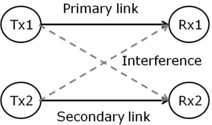
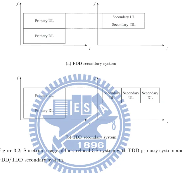
We consider a hierarchical underlying CR system, consisting of a primary system and secondary system. The primary system owns a licensed spectrum. The secondary system aims to provide services to secondary users under the condition that it can not interfere with the primary system. In the fourth generation (4G) of cellular wireless standards, the frequency division duplex (FDD) and time division duplex (TDD) are both considered. Therefore, what kind of duplexing modes of the primary and secondary is most suitable for hierarchical underlying CR system should be discussed. If the primary system is TDD, the secondary system may interfere primary downlink and uplink in one transmission time for both TDD and FDD secondary systems as shown in Fig. 3.1. The interference to primary system would hardly be managed. If the primary system is FDD, the secondary systems can transmit at the primary downlink or uplink spectrum. The secondary system utilizing the uplink spectrum of primary users is a better option for two reasons. First, the quality of service (QoS) requirement of uplink is usually less strict than downlink. Thus, it may endure larger interference from secondary system. Secondly, in order to cancel the interference, the channel state information (CSI) of the entire system must be known at the secondary base station. If secondary system utilize the uplink spectrum of primary system, the channels from primary users can be estimated directly. If utilizing downlink spectrum, on the other hand, the CSI estimation would become indirect. Therefore, secondary

Primary DL f Primary UL Primary DL f Secondary DL Secondary UL Secondary DL t t

(a) TDD secondary system

Secondary UL Secondary DL Primary DL f Primary UL Primary DL t f t (b) FDD secondary system

Figure 3.1: Spectrum usage of hierarchical CR system with FDD primary system and TDD/FDD secondary system.

system underlying the primary uplink spectrum is considered as shown in Fig. 3.2. To summarize, FDD primary system and TDD secondary system utilizing the primary uplink spectrum is considered in the thesis.

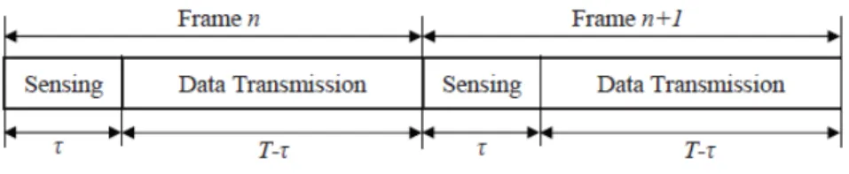
In order to avoid interference to primary systems, spectrum sensing is an im-portant functionality required in a CR system. Cognitive radio frame structure has been defined by IEEE 802.22. Each radio frame consisting of sensing period and data transmission period is shown in Fig. 3.3. In the sensing period, the CR system should stop transmission and receive the signal from primary system. Thus, the cognitive receiver can detect the existence of primary transmitters and estimate channel of the

Secondary DL Secondary UL t f Primary UL t f Primary DL

(a) FDD secondary system

t f Secondary DL Primary UL t f Primary DL Secondary DL Secondary UL (b) TDD secondary system

Figure 3.2: Spectrum usage of hierarchical CR system with TDD primary system and FDD/TDD secondary system.

transmitters. We assume the channels between primary users and the secondary base station can be estimated in the sensing period if the two systems are synchronized. Besides, the secondary base station can overhear the control channel of the primary system. So, the secondary base station knows the channels of PU-SBS and SU-SBS links perfectly. In addition to the above description, we assume that the secondary base station also knows the CSI of SU-PBS links which is much difficult to be realized. It can be achieved if the primary base station has the spectrum sensing ability and

Figure 3.3: Cognitive radio frame structure in IEEE 802.22.

cooperates with the secondary base station. The other way is that secondary base station uses statistic channel model of the area to estimate the SU-PBS channels by knowing the locations of secondary users and primary base station.

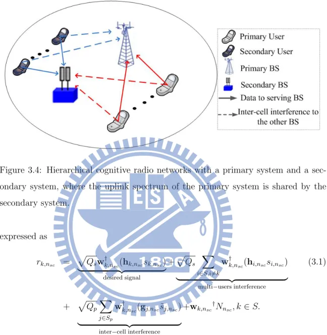
The uplink channel model of hierarchical underlying CR system with primary system and secondary system is shown in Fig. 3.4. Primary users and the secondary users are equipped with single antenna. Each of the secondary and primary base station is equipped with M antennas. The secondary BS serve M secondary users at the most, which is selected from K secondary users, where K > M . The secondary base station has global CSI information of the entire CR system.

3.1

Signal Model for Multi-Carrier Hierarchical

Cognitive Radio System

Since a OFDM symbol encodes data on multiple orthogonal narrow band subcarriers, we can process the signal in the frequency domain and obtain desirous data on each subcarrier of which the channel is flat fading. Let sk,nsc and ˜sk,nsc denote the

trans-mitted signals from k-th secondary user to the secondary BS and k-th primary user to the primary BS, respectively. An M× 1 vector wk,nsc represents beamforming weight

for the k-th secondary user. S is the set of served users, where S ⊆ {1, · · · , K}. Then, the received signal of the k-th secondary user on the nsc-th subcarrier can be

Figure 3.4: Hierarchical cognitive radio networks with a primary system and a sec-ondary system, where the uplink spectrum of the primary system is shared by the secondary system. expressed as rk,nsc = √ Qsw†_k,nsc(hk,nscsk,nsc) | {z } desired signal +√Qs ∑ i∈S,i̸=k w†_k,nsc(hi,nscsi,nsc) | {z }

multi−users interference

(3.1) + √Qp ∑ j∈Sp w†_k,n sc(gj,nsc˜sj,nsc) | {z }

inter−cell interference

+wk,nsc

†_N

nsc, k∈ S.

where hk,nsc denotes channel between M antennas of secondary BS and the k-th

secondary user, √Qp and

√

Qs denote the transmit power of the primary user and

the secondary user on a subcarrier respectively, gk,nsc denotes MIMO channel vector

between secondary BS and k-th primary user, Sp is the set of scheduled primary

users, and N is a Gaussian noise for secondary BS with zero mean and variance σ2

N.

received signal at the primary BS can be written as following by exchange sk,nsc and ˜ sk,nsc properly: ˜ rk,nsc = √ Qpw˜_k,n† _sc(˜hk,nscs˜k,nsc) | {z } desired signal +√Qp ∑ i∈Sp,i̸=k ˜ w†_k,n sc(˜hi,nscs˜i,nsc) | {z }

multi−users interference

(3.2) + √Qs ∑ j∈S ˜ w†_k,n sc(˜gj,nscsj,nsc) | {z }

inter−cell interference

+ ˜w†_k,n

sc

˜

Nnsc, k ∈ S.

where ˜hk,nsc and ˜gk,nsc denote the MIMO channel vector of k-th primary user and

secondary user to the primary BS respectively. ˜N is the Gaussian noise for primary BS.

We assume that the average power of signal E[|sk,nsc|

2]

and E[|˜sk,nsc|

2]

is normalized to one. Thus, according to (3.1) the received signal SINR for the k-th secondary user in the nsc subcarrier is given by

γk,nsc = Qsw†k,nschk,nsc  2 Qs ∑ i∈S,i̸=k  wk,n† schi,nsc  2+ Qp ∑ j∈Sp  w†k,nscgj,nsc  2+ σ2 N . (3.3)

Similarly, the SINR of primary user k is derived by (3.2) as:

˜ γk,nsc = Qp ˜w†_k,nsch˜k,nsc  2 Qp ∑ i∈Sp,i̸=k   ˜w†_k,nsch˜i,nsc  2+ Qs ∑ j∈S   ˜w†_k,nscg˜j,nsc  2+ ˜σ2 N . (3.4)

If there is no ISI, then we can design beamforming weights at each subcarrier to cancel the interference on the denominator.

3.2

Performance Metrics

3.2.1

System Sum Rate

We consider a multi-user MIMO system, and utilize Shannon capacity formula to model the system sum rate as follows:

Csum =

∑

k∈S

log₂(1 + γk) , (3.5)

where S is the set of served users in each transmission; γk is the signal to

interfer-ence and noise ratio (SINR) of the k-th user. The sum rate of secondary system is considered as the main performance metric in our work.

3.2.2

Interference Power and Channel Correlation

For a hierarchical CR system, the interference to the primary system should be limited strictly. According to (3.4) the inter-cell interference power for the primary BS to receive i-th PU’s signal on subcarrier nsc:

PICI(i, nsc) = Qs ∑ j∈S   ˜w†_i,nscg˜j,nsc  2 (3.6)

Therefore, we can set appropriate transmit power for scheduled secondary users to limit the inter-cell interference (ICI) shown in (3.6) to any predefined threshold through simulation. Moreover, we design a scheduling algorithm to lower the in-terference while choosing the users who have better CSI for the secondary BS. It is very common to schedule users by the orthogonality of channel vectors in multi-user MIMO system. It is more likely to distinguish data through receive beamforming when the channel vectors of different users are more unalike. A metric called channel correlation is defined in [8] to evaluate the orthogonality between two channel vectors

h and g:

Ω(h, g) = h

†_g

We will use this metric to estimate the influence of a certain secondary user on the served primary users and decide which secondary user can be selected.

3.3

Problem Formulation

In this thesis, we tried to solve the interference control problem at secondary BS. The secondary BS should schedule secondary users to make the interference to primary BS as small as possible. When receiving the data from served users, the secondary BS uses beamforming technique to cancel the interference from concurrent primary users. Based on the signal model and performance metric described in Section 3.1 and 3.2, the single carrier transmission can be regarded as a special case in multicar-rier transmissions. Therefore, the following problems are formulated in multicarmulticar-rier transmissions. Before data transmission, the secondary BS should know the CSI from scheduled primary users and all the secondary users to the primary BS in each uplink resource block. Then, the secondary BS schedules users whose MIMO channel vector is near orthogonal to the scheduled primary users’ receive beamforming weights.

S = {j| ˜wi,nsc⊥˜gj,nsc, i∈ Sp, nsc ∈ [1, Nsc], j = 1, ..., K}, |S| ≤ M . (3.8)

where Nsc is the amount of subcarriers in one resource block, K is the amount of

secondary users requiring for service, and M is the number of receive antennas on secondary BS. The symbol ”⊥” represents near-orthogonal here. After knowing the scheduled users in the hierarchical CR system, the sum rate maximization beamform-ing problem for the secondary network is formulated as follows:

Csum = max

wi,1,...,wi,Nsc

N∑sc

nsc=1

∑

i∈Slog2(1 + γi,nsc) , (3.9)

s.t.∥wi,nsc∥ ≤ 1 .

22

CHAPTER 4

Quasi-Convex Beamformer Design

In this chapter, we present a joint beamforming and scheduling design to make the MIMO-OFDM hierarchical CR system have good performance. A receive beamform-ing problem is proposed to maximize the sum-rate of the secondary system when knowing the users served in each system. It is transferred to a quasi-convex problem. An iterative algorithm is proposed to choose the secondary users who have better channel condition and relatively cause less interference to the primary system.

4.1

Sum-Rate Maximization Receive

Beamform-ing

In this thesis, the goal of using MIMO beamforming technique at secondary base station is to maximize the sum-rate shown in (3.3). As we can see from (3.3), the objective function is the sum of capacity of every scheduled users on a designated group of subcarriers. Since a receive beamforming problem is considered here, the beamforming weights for a user don’t cause any effect on the other users’ signal, which is not like transmit beamforming. Due to this feature, the original optimization problem can be decomposed into many sub-problems to maximize the capacity of each

user as problem (4.1).

max

wi,1,...,wi,Nsc,∥wi,nsc∥≤1

Nsc ∑ nsc=1 ∑ i∈S log₂(1 + γi,nsc) ≡ max

wi,1,...,wi,Nsc,∥wi,nsc∥≤1

Nsc

∑

nsc=1

log₂(1 + γi,nsc),∀i ∈ S. (4.1)

Moreover, the multi-carrier signal can be processed in frequency domain and the subcarrier are orthogonal, so the beamforming weights for each user on each subcarrier can be determined by solving the optimization problem in (4.2).

max

wi,1,...,wi,Nsc,∥wi,nsc∥≤1

N∑sc

nsc=1

log₂(1 + γi,nsc),∀i ∈ S

≡ max

wi,nsc,∥wi,nsc∥≤1

log₂(1 + γi,nsc),∀i ∈ S, nsc ∈ [1, Nsc]. (4.2)

The objective function in (4.2) is log₂(1 + γi,nsc). Because log function is

mono-tonic increasing, which means the output value is maximized when the input variable reaches its maximum value, the capacity maximization problem can be simplified fur-ther into an SINR maximization problem, i.e.maximizing the variable γi,j by deciding

the beamforming weights for each subcarrier of every users.

w⋆_i,nsc = arg max γi,nsc,

= arg max wi,nsc Qsw†i,nschi,nsc  2 Qs ∑ k∈S,k̸=i  w†i,nschk,nsc  2+ Qp ∑ l∈Sp  w†i,nscgl,nsc  2+ σ2_N , (4.3) ∥wi,nsc∥ ≤ 1, ∀i ∈ S, nsc ∈ [1, Nsc].

The above optimization problem is not convex since the variable wi,j is on the

nom-inator and denomnom-inator of the objective function simultaneously. It will be showed that this problem can be transformed into a quasi-convex problem in the following subsection.

4.2

Convexity of Beamforming Problem

Before transform the original problem into a equivalent solvable form, some definitions of the reformulation technique we used are given.

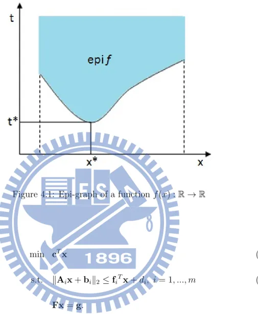
Epigraph reformulation: An epigraph of a function f :Rn→ R is a set of points in

Rn+1 _{domain lying on or above its graph. Every optimization problem has a general}

epigraph form by introducing a new variable t representing the output value of the objective function. The epigraph form of a typical optimization problem is defined in problem (4.4). A simple diagram expressing the meaning of epigraph reformulation is shown in Fig. 4.1, where the objective function f is R → R.

min f0(x) s.t. fi(x)≤ 0, i = 1, ..., m hi(x) = 0, i = 1, ..., p ≡ min t (4.4) s.t. f0(x)≤ t fi(x)≤ 0, i = 1, ..., m hi(x) = 0, i = 1, ..., p.

Second order cone programming: There are many function or sets of vectors are

known for its convexity in their domain of definition. Here, we introduce a convex set inRn+1 _{called second order cone. It has a specific form: K =}{(x, t) ∈ Rn+1| ∥x∥

2 ≤

t}. Its shape in R3 _{space is shown in Fig. 4.2. Because of the convexity of a second}

order cone, a specific form of optimization problem called second order cone program-ming comes up as problem (4.5), which is a convex optimization problem.

Figure 4.1: Epi-graph of a function f (x) :R → R

min cTx (4.5)

s.t. ∥Aix + bi∥2 ≤ fiTx + di, i = 1, ..., m (4.6)

Fx = g.

where Ai ∈ Rni×n, bi ∈ Rni×1, fi ∈ Rn×1. The feature of SOCP is that each

inequality constraints involves a generalized inequality defined by a second order cone

Ki ={(x, t) ∈ Rni+1| ∥x∥2 ≤ t}, i.e. (Aix + bi, fiTx + di)∈ Ki. Since x in constraint

set i are mapped onto a convex set Ki through affine mapping, constraint set i is

proven to be convex. The objective function and the equality constraints are just linear combinations of the elements in x which are convex obviously. Thus, if an optimization problem can be transformed to a SOCP, it is solvable and a global

Figure 4.2: A typical second-order cone in R3

optimal is guaranteed. So far, the discussions in this section focus on functions in domain of real numbers, but the definitions of SOCP and epigraph reformulation is same the domain of problem is expanded to complex numbers (i.e. replace R by C). The above definitions for problem reformulation are used for our beamforming problem which is in the domain of complex numbers.

Quasi-convex functions: A real valued function f (x) is quasi-convex if each of

sub-level set Sα(f ) = {x|f(x) ≤ α} is a convex set for every α. The negative of a

quasi-convex function is said to be quasi-concave. f (x) is quasi-concave if Sα(−f) =

{x|f(x) ≥ α} is convex for every α. The objective function of beamforming problem in (4.3) is quasi-concave, which can be proved by the definition of quasi-concave functions:

where f (wi,nsc) = Qswi,n† schi,nsc  2 Qs ∑ k∈S,k̸=i  w†i,nschk,nsc  2+ Qp ∑ l∈Sp  w†i,nscgl,nsc  2+ σ_N2 , =⇒ f(wi,nsc)≥ α ≡ Qsw†i,nschi,nsc  2 ≥ α ( Qs ∑ k∈S,k̸=i  w†i,nschk,nsc  2+ Qp ∑ l∈Sp  w†i,nscgl,nsc  2 + σ2 N ) . (4.8)

(4.8) will be proved to be a second order cone in Cn+m+2 _{from (4.9) to (4.11):}

Qsw†i,nschi,nsc  2 ≥ α ( Qs ∑ k∈S,k̸=i  w†i,nschk,nsc  2 + Qp ∑ l∈Sp  wi,n† scgl,nsc  2+ σ2 N ) (4.9) ≡ (1 + 1_{α )}h†_i,nscwk,nsc  2 ≥ ∑ k∈S  h†i,nscwk,nsc  2+Qp Qs ∑ l∈Sp  g†i,nscwl,nsc  2+ σ 2 N Qs (4.10)

≡ ∥Ai,nscwi,nsc+ b∥2 ≤

√ 1 + 1/αh†_i,n scwk,nsc (4.11) Ai,nsc = [ h1,nsc, ..., hn,nsc, √ Qp Qsg1,nsc, ..., √ Qp Qsgm,nsc, 01×M ]† b = [01×(n+m),√σN Qs ]T_.

Starting with (4.9), we add Qsti,nsc

w†i,nschi,nsc

2 on both side of (4.9) and divide both side by Qsti,nsc. After a transposition process, the inequality becomes (4.10). Finally,

the original inequality constraint is transformed into a form, which is similar to second order cone, by taking the square root on both side and introducing a channel matrix

Ai,nsc and a noise vector b. As shown in (4.11), for every α, the sub-level set is

like (4.6) which is a second order cone constraint and is convex. So, this objective function is a concave function. The minimum value of a quasi-convex function can be converged by iterative bisection algorithm (if one exists). On the other hand, the maximum value of a quasi-concave function can be converged too.

4.3

Beamforming Algorithm

Now, we begin the transformation of (4.3). The optimal beamforming weight for subcarrier nsc of SU i can be obtained by solving problem (4.12) and its epigraph

form is written as problem (4.13). Next, we should change the inequality constraint in (4.13) into a convex one.

max wi,nsc,∥wi,nsc∥≤1 Qswi,n† schi,nsc  2 Qs ∑ k∈S,k̸=i  wi,n† schk,nsc  2+ Qp ∑ l∈Sp  w†i,nscgl,nsc  2+ σ_N2 (4.12) ≡ max

wi,nsc,ti,nsc,∥wi,nsc∥≤1

ti,nsc (4.13) s.t. Qsw†i,nschi,nsc  2 Qs ∑ k∈S,k̸=i  w†i,nschk,nsc  2+ Qp ∑ l∈Sp  w†i,nscgl,nsc  2+ σ2_N ≥ ti,nsc.

Note that the constraint in (4.13) is same as (4.9) by just changing α into ti,nsc.

Therefore, it can be reformulated into a convex one by taking the same procedure from (4.9) to (4.11): Qsw†i,nschi,nsc  2 ≥ ti,nsc ( Qs ∑ k∈S,k̸=i  wi,n† schk,nsc  2+ Qp ∑ l∈Sp  w†i,nscgl,nsc  2+ σ2_N ) (4.14) ≡ (1 + _t 1 i,nsc )h†_i,n scwk,nsc  2 ≥ ∑ k∈S  h†i,nscwk,nsc  2+Qp Qs ∑ l∈Sp  g†i,nscwl,nsc  2+σ 2 N Qs (4.15)

≡ ∥Ai,nscwi,nsc+ b∥2 ≤

√ 1 + 1/ti,nsch † i,nscwk,nsc (4.16) Ai,nsc = [ h1,nsc, ..., hn,nsc, √ Qp Qsg1,nsc, ..., √ Qp Qsgm,nsc, 01×M ]† b = [01×(n+m),√σN Qs ]T_.

For fixed ti,nsc, the above constraint of the optimization problem is a second-order cone

of SOCP using bisection method. The original SINR maximization beamforming problem becomes:

max

wi,nsc,ti,nsc,∥wi,nsc∥≤1

ti,nsc (4.17)

s.t.∥Ai,nscwi,nsc + b∥2 ≤

√ 1 + 1/ti,nsch † i,nscwk,nsc. Ai,nsc = [ h1,nsc, ..., hn,nsc, √ Qp Qsg1,nsc, ..., √ Qp Qsgm,nsc, 01×M ]† b = [01×(n+m),√σ_QN_s]T ∀i ∈ S, nsc ∈ [1, ..., Nsc].

Bisection method is a way to search for the root of a continuous function by dichotomy. The bisection method is used to find the optimal value of the beamforming problem (4.17) and the algorithm is as follows:

1. Set the expected SINR upper bound u and lower bound l: u := 104 _{and l := 0.}

Set the convergence tolerance: ϵ := 1.

2. For i = 1 :|S|, for nsc = 1 : Nsc; while u− l ≥ ϵ :

(a) ti,nsc := (l + u)/2.

(b) Solve the convex problem (4.17).

(c) if the problem is solvable, l := ti,nsc; otherwise u := ti,nsc.

When we set a small number of error tolerance ϵ, and set the bounds properly, i.e.

l ≤ t⋆_i,nsc ≤ u, the bisection algorithm can find a solution close to the global optimal

enough. One thing needs to be mentioned is that the convex problem (4.17) is solved by the CVX Matlab toolbox [1].

30

CHAPTER 5

Channel Dependent Multi-User

Scheduling

5.1

Proposed Channel Dependent Scheduling

Al-gorithm

So far, the secondary base station is able to have the best signal quality for every scheduled UE using MIMO beamforming technology. The next challenge is how to select a set of UEs which have good channel condition and cause less interference to the primary base station. In order to minimize the interference power to the primary BS, we should focus on the inter-cell interference term of the signal model for primary receive signal. The inter-cell interference power on i-th primary user’s nsc-th subcarrier is formulated in subsection 3.2.2, equation (3.6):

PICI(i, nsc) = Qs ∑ j∈S   ˜w†_i,nscg˜j,nsc  2. (5.1) where ˜w†_i,n

sc represents primary user i’s receive beamforming weights on subcarrier

nsc. ˜gj,nsc denotes the MIMO channel vector of j-th SU to PBS link on subcarrier

nsc. S are the set of scheduled PUs and SUs. In order to avoid serious interference to

primary system, the secondary BS should choose a set of SUs so that PICI is smaller

beam-forming vector, ˜w†_i,nsc, for i-th scheduled primary user’s nsc-th subcarrier is unknown

for secondary BS. But the secondary BS can assume that the beamforming weight is determined by ideal zero-forcing beamforming (ZFBF) method which takes the chan-nel vectors of PUs in Sp into account. The orthogonality of channel vectors plays an

important role in MIMO beamforming. For the beamforming vector of PU i ( ˜wi,nsc),

it will have the following property: ˜wi,nsc ∥ ˜hi,nsc and ˜wi,nsc ⊥ ˜hj,nsc,∀j ̸= i, j ∈ Sp.

If the scheduled SU’s channel vector is nearly parallel to the beamforming vector of i-th primary user, ˜w_i,n† _sc is unable to null the interference signal, which will cause great interference. Therefore, we should choose SUs whose channel vectors to the pri-mary BS is nearly orthogonal to scheduled PUs’ beamforming vectors. The channel correlation metric for PU i and SU j on subcarrier nsc is defined as:

Ωnsc

i,j =

| ˜w†_i,nscg˜j,nsc|

∥ ˜wi,nsc∥∥˜gi,nsc∥

. (5.2)

The value of this metric is between 0 to 1. The smaller the value is, the two vectors are more orthogonal. Besides the orthogonality of vectors, the pathloss effect also affect the value of inner product: ˜wi,nscg˜j,nsc =∥ ˜wi,nsc∥∥˜gj,nsc∥ cos θ. For instance, although

SU j has a highly correlative channel with PU i, on the condition that its location is far away from the primary BS, its signal also causes little interference. This scenario can’t be discovered by the ordinary channel correlation metric in (5.2) because the channel gain is divided by the denominator. We introduce a upper bound of channel gain ”gd” here, which will be used in the scheduling algorithm. gdrepresents the gain

of pathloss effect for SU-PBS link. It can be set as ρ−Qsin dB, where ρ in dBm is the

ICI power constraint for each subcarrier and Qs in dBm is secondary users’ transmit

power on each subcarrier. If the channel gain of a SU is less than gd, it is expected to

cause ICI power less than ρ dBm to the primary system on each subcarrier. Assume there are K SUs requiring for service. In a specific resource block, a set of PUs called Sp is about to transmit data concurrently. User scheduling in the resource block

with Nsc subcarriers is considered here. Before introducing the scheduling algorithm,

we define two functions which will be used afterwards. Firstly, the average channel correlation metric for SU i and SU j on a resource block:

ωi,j = 1 Nsc Nsc ∑ nsc=1  h†i,nschj,nsc   ∥hi,nsc∥ ∥hj,nsc∥ . (5.3)

where h represents the channel vector of SU-SBS link. Secondly, the average channel gain in step (3) is:

G(i) = 1 Nsc Nsc ∑ nsc=1 ∥hi,nsc∥. (5.4)

The following is the proposed user schedule algorithm:

1. Set an orthogonality tolerance δ := 0.1 and ICI power threshold ρ :=−120 dBm.

2. ∀j ∈ [1, K] :

If the channel gain∥˜gj,nsc∥

2 _{≤ g}

d,∀nsc, SU j is put into a candidate set S′, else:

(a) Calculate the channel correlation metric between SU j and every PU i∈ Sp on

all the subcarriers in the resource block.

(b) Find the maximum value of all the correlation metrics in one resource block: Ωmax

j = max_i,n

sc

Ωnsc

i,j

(c) Put SU i, whose Ωmax_j ≤ δ, into a set S′ Finally the candidate set becomes:

S′ ={j|∥˜gj,nsc∥

2 _{≤ g}

d,∀nsc} ∪ {j|Ωmaxj ≤ δ}.

3. Sort the element in S′ by the average channel gain G(i) in descent order i.e.

G(S′(1))≥ G(S′(2))≥ ... ≥ G(S′(|S′|)).

5. While |S| < M ∧ PICI(k, nsc) < ρ,∀k ∈ Sp: Refresh S = S∪ S′(i⋆), i⋆ = max i∈S′,S′(i) /∈S ( G(i)/∑ j∈S ωS′(i),j ) .

In the above algorithm, we set δ := 0.1 to ensure the selected SUs whose channel is near-orthogonal to the PUs. After choosing the qualified SUs who will cause less interference to the primary system, we select the secondary user with best CSI into set S first. Then, we select the one who have better channel gain, and average channel correlations ω between it and those in S must be small relatively. Before adding a qualified SU, we should check if the inter-cell interference (ICI) power exceed the threshold ρ. This threshold is about 10 dB to the noise power (-132 dBm) on the bandwidth of one subcarrier. The value of ρ is acceptable for our system scenario since SNR for primary users are 40 dB on average in our pre-simulation.

In order to promote the overall spectrum efficiency in CR systems, the sacrifice of primary system’s performance is inevitable. The secondary system is responsible to control the interference and ensure the QoS of primary users. The basic idea of proposed scheduling scheme is to control the interference power under a threshold. The effectiveness of our scheduling scheme will be proved by comparing with some optimal scheduling schemes which are very complicated. The performance of proposed scheme is close to the optimal scheme in simulation results.

5.2

Random and Optimal Scheduling Scheme

Since the proposed scheduling algorithm is suboptimal. We need to evaluate the effec-tiveness of the proposed scheme. In this section, we introduce three other scheduling schemes and the performance of all the scheduling schemes will be compare in chap-ter 6. The first scheme is selecting M SUs randomly from the candidate SUs. This scheme is the simplest and is esteemed as a lower bound in performance

son. Secondly, an optimal scheduling scheme, which is dedicated to maximizing the throughput of primary system, is taken into account. The optimal solution is gotten by solving problem (5.5). The optimal solution guarantees that the scheduled SUs cause least affection to primary system in a resource block. Because problem (5.5) is a 0-1 integer programming problem which is NP hard, we can solve the problem by exhaustive search. This ICI-minimizing scheduling scheme will be combined with our quasi-convex beamforming algorithm and the throughput performance will come up in chapter 6. max S Nsc ∑ nsc=1 ∑ i∈Sp log₂(1 + ˜γi,nsc) (5.5)

s.t. |S| = M, PICI(i, nsc)≤ ρ, ∀i, nsc

where ˜γi,nsc = Qp ˜w†i,nsc ˜ hi,nsc  2 Qp ∑ j∈Sp,j̸=i   ˜w†_i,nsch˜j,nsc  2+ Qs ∑ k∈S   ˜w_i,n† _scg˜k,nsc  2+ ˜σ_N2 .

The beamforming weights for PUs considered in problem (5.5) are decided by ZFBF technique previously. If (5.5) is unsolvable, which means the optimal user set of M SUs cause ICI power greater than the constraint, we should reduce the number of served SUs (i.e. M = M − 1) and solve (5.5) again. Finally, we also discuss a scheduling scheme for sum rate maximization. This scheduling scheme takes the beamforming technique of each cell into consideration and select the SUs to maximize the system sum rate. Since this scheme guarantees the maximum sum rate, it is esteemed the upper bound for all the scheduling scheme. The optimization problem is shown in problem (5.6). The optimal solution is obtained by exhaustive search.

max S,wj,nsc Nsc ∑ nsc=1  ∑ i∈Sp log₂(1 + ˜γi,nsc) + ∑ j∈S log₂(1 + γj,nsc)   , s.t. |S| = M. (5.6)

where ˜γi,nsc = Qp ˜w†i,nsc ˜ hi,nsc  2 Qp ∑ k∈Sp,k̸=i   ˜w†_i,nsch˜k,nsc  2+ Qs ∑ j∈S   ˜w†_i,nscg˜j,nsc  2+ ˜σ2_N γj,nsc = Qswj,n† schj,nsc  2 Qs ∑ k∈S,k̸=j  w†j,nschk,nsc  2+ Qp ∑ i∈Sp  wj,n† scgi,nsc  2+ σ2_N . ˜

γi,nsc is the throughput of primary user i on nsc-th subcarrier and γj,nsc is the

through-put for secondary user j. Note that the optimal beamforming weights for SUs should be decided by quasi-convex algorithm every time when the different set of scheduled SUs is considered.

36

CHAPTER 6

Simulation Results

6.1

Assumptions

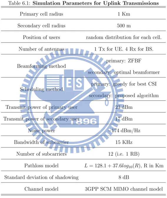
In this subsection, we describe the simulation environments for evaluating the perfor-mance of proposed beamforming and scheduling algorithm. We establish a hexagon primary cell with l kilo-meter radius and a smaller secondary cell of 500 meter ra-dius overlapping with the primary cell. The position relationship of the two cells is illustrated in Fig.6.1. For approaching real circumstance, we use the MIMO spa-tial channel model (SCM) for urban macro cell, specified by 3GPP work group TR 25.996 [18]. The pathloss, shadowing effect, and the subcarrier spacing are set accord-ing to 3GPP TR 36.814 [19] for 2 GHz carrier frequency and 10MHz bandwidth. For simulation and evaluation convenience, we only allocate the first resource block for uplink signalling and perform the signal processing. Fairness is not considered here. The primary BS select 4 users with best channel gain simultaneously and implement zero-forcing beamforming. The secondary BS executes the proposed scheduling and beamforming technique. The detail simulation parameters are listed in Table 6.1.

Table 6.1: Simulation Parameters for Uplink Transmissions

Primary cell radius 1 Km

Secondary cell radius 500 m

Position of users random distribution for each cell. Number of antennas 1 Tx for UE. 4 Rx for BS.

Beamforming method

primary: ZFBF

secondary: optimal beamformer

Scheduling method

primary: greedy for best CSI secondary: proposed algorithm

Transmit power of primary user 23 dBm

Transmit power of secondary user 17 dBm

Noise power −174 dBm/Hz

Bandwidth of subcarrier 15 KHz

Number of subcarriers 12 (i.e. 1 RB)

Pathloss model L = 128.1 + 37.6log10(R), R in Km

Standard deviation of shadowing 8 dB

Channel model 3GPP SCM MIMO channel model

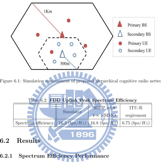
Figure 6.1: Simulation environment of proposed hierarchical cognitive radio network

Table 6.2: FDD Uplink Peak Spectrum Efficiency

Simulator 3GPP rel.8 ITU-R

1× 4 SIMO reqirement

Spectrum efficiency 16.2 (bps/Hz) 16.8 (bps/Hz) 6.75 (bps/Hz)

6.2

Results

6.2.1

Spectrum Efficiency Performance

The system performance of our proposed CR system is shown in this subsection. We assume that there are N UEs requiring for uplink service in each cell. Although the number of users may be different in different cell and at different time in reality, we set N = 50 in each cell at each time slot, to see the general performance of the proposed algorithms. For the secondary system, N = 50 is large enough to schedule M (= 4) SUs simultaneously. In each simulation process, we spread N UEs randomly in the domain of each cell. Then, we perform the beamforming and and scheduling

0 5 10 15 20 25 0 0.1 0.2 0.3 0.4 0.5 0.6 0.7 0.8 0.9 1 Spectrum efficiency (bps/Hz/UE) CDF Primary−ordinary Primary−CR Secondary−CR Primary+secondary

Figure 6.2: CDF plot for UEs’ spectrum efficiency of the CR system, where proposed BF and scheduling algorithm is adopted.

algorithm in Table 6.1 and get the capacity for each scheduled user. Since fairness is not considered here, the PUs with best CSI is chosen in each simulation round, which means that the outcome represents the peak spectrum efficiency of the system. The peak spectrum efficiency of the ordinary primary cell, which doesn’t coexist with secondary cell, is compared with the 3GPP calibration result in Table 6.2. The value is very similar and achieves the ITU-R requirement. This shows the validity of the simulator. We obtain the experimental CDF plot of UE’s throughput distribution in Fig. 6.2 after 200 independent rounds. From Fig. 6.2, it is found that the addition of secondary cell causes little performance degradation of primary system, but the additional throughput of secondary system is much more than the decreased quantity of primary system’s. In order to see the gain of spectrum efficiency brought from

0 5 10 15 20 25 30 0 0.1 0.2 0.3 0.4 0.5 0.6 0.7 0.8 0.9 1 Spectrum efficiency (bps/Hz) CDF Primary−ordinary Random+ZFBF Scheduling+ZFBF Proposed scheduling +BF

Figure 6.3: CDF for spectrum efficiency of the CR system, where the secondary BS schedules users randomly/sub-optimally while using ZFBF/quasi-convex technique.

secondary system, the spectrum efficiency of each PU in each simulation round is added by one corresponding SU. The spectrum efficiency of PUs and SUs are arranged in decreasing order, respectively, in advance. Those with the same order are summed up. This value stands for the spectrum efficiency which the CR system can achieved while a primary user is served.

For the purpose of performance comparison between beamforming schemes, we establish a scenario where secondary BS selects users by our scheduling algorithm and perform ZFBF on receive signal of scheduled users. The other more simplified sce-nario is introduced to be a worst case, where the secondary BS selects users randomly and adopts ZFBF for scheduled SUs. The CDF of CR system’s spectrum efficiency for different schemes are compared in Fig. 6.3. The statistics of spectrum efficiency