A genetic algorithm with disruptive selection

299 IEEE TRANSACTIONS ON SYSTEMS, MAN, AND CYBERNETICS-PART B: CYBERNETICS, VOL. 26, NO. 2, APRIL 1996

Correspondence

A

Genetic Algorithm with Disruptive Selection

Ting Kuo and Shu-Yuen Hwang

Abstruct-Genetic algorithms are a class of adaptive search techniques based on the principles of population genetics. The metaphor underlying genetic algorithms is that of natural evolution. Applying the “survival-of- the-fittest” principle, traditional genetic algorithms allocate more trials to above-average schemata. However, increasing the sampling rate of schemata that are above average does not guarantee convergence to a global optimum; the global optimum could be a relatively isolated peak or located in schemata that have large variance in performance. In this paper we propalse a novel selection method, disruptive selection. This method adopts a nonmonotonic fitness function that is quite different from traditional monotonic fitness functions. Unlike traditional genetic algorithms, this method favors both superior and inferior individuals. Experimental results show that GA’s using the proposed method easily find the optimal solution of a function that is hard for traditional GA’s to optimize. We also present convergence analysis to estimate the occurrence ratio of the optima of a deceptive function after a certain number of generations of a genetic algorithm. Experimental results show that GA’s using disruptive selection in some occasions find the optima more quickly and reliably than GA’s using directional selection. These results suggest that disruptive selection can be useful in solving problems that have large variance within schemata and problems that are GA-deceptive.

diag (V) 0 g F Hi > R , t H j I NOMENCLATURE Absolute matrix of a matrix

M.

Defining length of hyperplane H (the length of the smallest segment containing all the defining loci of

H ) .

Diagonal matrix of a vector V.

Occurrence matrix that represents the probabil- ity that each kind of string occurs at generation ! I .

];unction vector that represents the function values for each kind of string.

Average value of the objective function of the individuals in the population P ( t ) .

Hyperplane of the search space.

Set of individuals that are in the population

P ( t ) and are instances of hyperplane H .

H , is dominated by H3 in the population P ( t ) . H , is more worth exploring than H3 in the ]population P ( t ) .

H , is more remarkable than H3 in the popula- tion P ( t ) .

Identity column vector with dimension ( I

+

1) x 1.

Length of the bit string.

Number of individuals in the set H ( t ) .

Expected number of individuals in the set H ( t ) .

Order of hyperplane H .

Manuscript received July 14, 1993; revised February 13, 1994, and January 19, 1995. This work was supported by the National Science Council, Republic of China, under Grant NSC 84-2213-E-009-012.

The authors are with the Institute of Computer Science and Information Engineering, National Chiao Tung University, Hsinchu 30050, Taiwan, ROC.

Publisher Item Identifier S 1083-44 19(96)02300-X.

TP ” t S T ( X , t )

Crossover rate. Mutation rate. Population at time t .

Selection vector that represents theprobability that each kind of string is selected at generation 9.

Transition matrix that represents the probability of being mutated under the mutation rate p m . Expected number of offspring reproduced by individual z at time t.

Growth rate of the set H ( t ) without the effect of crossover and mutation.

Fitness of the individual x.

Average fitness of the individuals in the set Average fitness of the individuals in the popu- lation P ( t ) .

H

(4.

I. INTRODUCTION

Genetic algorithms (GA’s) have been applied in many diverse areas, such as function optimization [7], the traveling salesman problem [ll], [14], scheduling [5], [30], neural network design [19], [27], system identification [23], vision [4], control [22], and machine learning [8], [9], [16]. Goldberg’s book [12] provides a detailed review of these applications. The fundamental theory of genetic algorithms was presented in Holland‘s pioneering book [20].

The principle behind genetic algorithms is essentially that of Dar- winian natural selection. According to Neo-Darwinism, the process of evolution can be classified into three categories: stabilizing selection, directional selection, and disruptive selection [26]. Stabilizing selec- tion is also called normalizing selection, since it tends to eliminate individuals vvith extreme values. Directional selection has the effect of either incireasing or decreasing the mean value of the population. In contrast, disruptive selection tends to eliminate individuals with moderate values. We will give a formal definition of each of the three types of selection later. All traditional GA’s can be viewed as

a process of evolution based on directional selection. However, in some cases, a current worse solution may have a greater chance of “evolving” toward a better future solution. Why discard these worse solutions rather than trying to exploit them? This idea motivates our research.

The notatlion of schema must be introduced first so that we may understand hiow genetic algorithms can direct the search toward high fitness regions of the search space. A schema is a set of individuals in the search( space. In most GA’s, the individuals are represented by fixed-length binary strings. In the case of a binary string, a schema can be expressed as a pattern that is defined over the alphabet (0, 1, * }

and describes a subset of strings with similarities at certain string positions. In the pattern of

a

schema, 1’s and 0’s are referred to as defining bits: the number of defining bits is called the order of that schema. The distance between the leftmost and rightmost defining bits is referred to as the defining length of a schema. For example, the order of **0*11**1 is 4, and its defining length is 6. A bit string

x is said to be an instance of a schema s if x has exactly the same 1083-4419/96$05.00 0 1996 IEEE

300 IEEE TRANSACTIONS ON SYSTEMS, M

bit values in exactly the same locations that are defining bits in s. For example, 00011 and 00110 are both instances of schema 00*1*, but neither 1001 1 nor 00000 is an instance of schema 00*1*. Since every string of length L is an instance of 2L schemata, its fitness gives some information about those schemata. Thus, while explicitly sampling strings, the GA implicitly samples schemata. Schemata can be viewed as defining hyperplanes in the search space. Usually, the terms schema and hyperplane are used interchangeably.

Since GA’s are not admissible (i.e., no guarantee for an optimal solution), it is important to reduce the possibility of some GA’s missing the optimal solution. GA’s may fail to locate the optima of a function for several reasons [25]:

1) The chosen embedding (i.e., choice of domain) may be inap- propriate.

2) The problem is deceptive (i.e., tends to contain isolated optima: the best points tend to be surrounded by the worst) that is provably misleading for the simple three-operator genetic algorithms [12].

3) The problem is not deceptive, but average fitnesses of schemata cannot be reliably estimated because the sampling error is too large.

4) Average fitnesses of schemata can be reliably estimated, but crossover destroys individuals which represent schemata of high utility.

In this paper, we will propose a novel selection method and show that this new method can be helpful in the second and the third cases. The paper is organized as follows. In Section

JI,

we give a simple review of genetic algorithm. Different types of fitness functions are described in Section 111. GA’s that use disruptive selection to solve a nondeceptive but GA-hard function are described in Section IV. Then, in Section V, we derive a deterministic model for convergence analysis and demonsrate that GA’s using disruptive selection are more reliable than GA’s using directional selection in solving a deceptive function. Finally, in Section VI, we conclude the paper with a discussion of our results.

11. GENETIC ALGORITHM

A. Background

One description of genetic algorithms is that they are iterative procedures maintaining a population of individuals that are candidate solubons to a specific problem. At each generation the individuals in the current population are rated for their effectiveness as solutions, and in line with these ratings, a new population of candidate solutions is formed using specific genetic operators [20].

The three primary genetic operators focused on by most researchers are selection, crossover, and mutation. These are described below.

1) Selection (or Reproduction): The population of the next gen- eration is first formed by using a probabilistic reproduction process. In general, there are two types of reproduction pro- cesses: generational reproduction and steady-state reproduction. Generational reproduction replaces the entire population with a new population. In contrast, steady-state 1291, [31], re- production replaces only a few individuals in a generation. Whichever type of reproduction is used, individuals with higher fitness usually have a greater chance of contributing to the generation of offspring. Several selection methods may be used to determine the fitness of an individual. Proportional selection 1121, [20], and ranking [2] are the main selection schemes used in GA’s. The resulting population is sometimes called the intermediate population. The intermediate population is

AN, AND CYBERNETICS-PART B: CYBERNETICS, VOL. 26, NO. 2, APRIL 1996

then processed using crossover and mutation to form the next generation.

2) Crossover: A crossover operator manipulates a pair of in- dividuals (called parents) to produce two new individuals (called offspring) by exchanging segments from the parents’ coding. By exchanging information between two parents, the crossover operator provides a powerful exploration capability. A commonly used method for crossover is called one-point crossover. Assume that the individuals are represented as binary strings. In one-point crossover, a point, called the crossover point, is chosen at random and the segments to the right of this point are exchanged. For example, let z1 = 101010 and x2 =

010100, and suppose that the crossover point is between bits 4 and 5 (where the bits are numbered from left to right starting at I). Then the offspring are y1 = 101000 and y2 = 010110.

Several other types of crossover operators have been proposed, such as two-point crossover, multi-point crossover 171, uniform crossover El], [29], and shuffle crossover [lo].

3 ) Mutation: By modifying one or more of the gene values of an existing individual, mutation creates new individuals, increasing the variability of the population. The mutation operator ensures that the probability of reaching any point in the search space is never zero.

In this paper, we restrict our attention to the selection operator.

B. Selection Strategies

The selection operator plays an important role in driving the search toward better individuals and maintaining high genotypic diversity in the population.

Grefenstette and Baker 1171 noted that in selection strategies the selection phase can be divided into the selection algorithm and the sampling algorithm. The selection algorithm assigns to each individual z a real number, called the target sampling Tate, t s r ( z , t ) ,

to indicate the expected number of offspring reproduced by z at time

t.

The sampling algorithm then reproduces, according to the target sampling rate, copies of individuals to form a new population. Most well-known selection algorithms use proportional selection, which can be described as

where U is the fitness function and

a(t)

is the average fitness of the

population P ( t ) . For each selection algorithm,

where

H

is a hyperplane, H ( t ) is the set of individuals that are in the population P ( t ) and are instances of hyperplane H , m [ H ( t ) ] is the number of individuals of the set H ( t ) , and t s r [ H ( t ) ] is the growth rate of the set H ( t ) without the effects of crossover and mutation.

Thus,

where

u[H(t)]

is the average fitness of the set

H ( t ) .

Several researchers have studied mechanisms that affect the selection bias. Grefenstette [ 151 showed the effect of different scaling mechanisms on selection pressure. Baker [3] and Schaffer 1281 studied how different selection mechanisms bias selection. Whitley and Kauth [3 11 introduced a parameter for directly controlling selection pressure.

IEEE TRANSACTIONS ON SYSTEMS, MAN, AND CYBERNETICS-PART B: CYBERNETICS, VOL. 26, NO. 2, APRIL 1996 301

Goldberg and Deb’s [13] study is an excellent reference on selection methods; it compares four selection schemes commonly used in modern genetic algorithms.

C. Schema Processing

The Schema Theorem ~201, [211, a well-known property of G A ’ ~ ,

is formed from (3). 1171.

schema Theorem: a genetic algorithm using a proportional selection algorithm, a one-point crossover operator, and a mutation holds:

the rapid decline of selective pressure, many forms of dynamic fitness scaling have been suggested [12], [15]. For example, a dynamic linear fitness function has the form

U(.) = u f ( z )

+

b ( t ) . (7) Two definitions concerning the selection strategy are described below Definition 1: A selection algorithm is monotonic if the following

(8) Dejnition 2. A fitness function is monotonic if the following condition is satisfied:

operator, for each hyperplane H represented in P ( t ) the following _{t s r ( z , )}

₅

_{t s r ( z , ) cs U ( Z , )}

_I

U(.,).

condition is satisfied:

Here,

M [ H ( t

+

l)] is the expected number of individuals that will be the instances of hyperplane H at time t

+

1 under the genetic algorithm, given that M [ H ( t ) ] is the expected number of individuals at time t ,

p , is the crossover rate, pm is the mutation rate,

d ( H ) is the defining length

o ( H ) is the order of hyperplane H , and

L is the length of each string.

The term

{ % [ H ( t ) ] / a

( t ) } denotes the ratio of the observed average fitness of the hyperplane

H

to the overall population average. This term determines the rate of change of M [ H ( t ) ] , subject to the “error” terms (1 - b c d ( H ) / L - 1 ] } ( 1 - p,)”(*). The term

M [ H ( t

+

l)] increase,; if E [ H ( t ) ] is above the average fitness of the population (when the error terms are small), and vice versa. The error terms denote the effects of breaking up instances of hyperplane

H caused by crossover and mutation. The term (1 - b c d ( H ) / L

-

l ] } { M [ H ( t ) ] } specifies an upper bound on the crossover loss, the loss of instances of H resulting from crosses that fall within the defining length d ( H ) of H . The term (1 - P , ) ’ ( ~ ) gives the proportion of instances (of

H

that escape a mutation at one of the o ( H )

defining bits of H . We can say that the Schema Theorem expressed

a reduced view of GA: only the effect of selection is emphasized, while the effects of crossover and mutation are presented as a negative role. In short, the Schema Theorem predicts changes in the expected number of individuals belonging to a hyperplane between two consecutive generations. Clearly, short, low-order, above-average schemata receive an exponentially increasing number of trials in subsequent generations,. However, increasing the sampling rate of schemata that are above-average does not guarantee convergence to a global optimum.

of hyperplane H ,

111. MONOTONIC VERSUS NONMONOTONIC FITNESS FUNCTIONS

The fitness function determines the productivity of individuals in a population. Clearly, the Schema Theorem is based on the fitness function rather than the objective function.

In general, a fitness function can be described as

4.)

=

s[f(z)l

( 5 )

where f is the objective function and U(.) is a nonnegative number.

The function g is often a linear transformation, such as

U(.) = u f ( z )

+

b (6)

where a is positive when maximizing f and negative when minimiz- ing f and b is used to (ensure a nonnegative fitness. In order to avoid

Here (and hereafter) a

=

1 when maximizing f and a = -1 when minimizing

f.

In this paper, we propose a nonmonotonic fitness function instead of a monotonic fitness function. A nonmonotonic fitness function is one for which (9) is not satisfied for some individuals in a population. A. Monotonic Fitness Functions

All traditional GA’s use monotonic fitness functions. Monotonic fitness functions do not provide good performance for all types of problems. Grefenstette and Baker [17] have stated the following two theorems to describe the search behavior of genetic algorithms in terms of the objective function.

Theorem 1: In any GA that uses a proportional selection algorithm and a dynamic linear fitness function, for any pair of hyperplanes

H,, H ,

in the population P ( t ) , if the average value of the objective function over the set H , ( t ) is less than that over the set H , ( t ) , then

H , will receive fewer trials than H, does.

Although tlhis theorem shows how to characterize the search behavior of a class of genetic algorithms in terms of the objective function, it still fails to cover many successful genetic algorithms, such as a genetic algorithm using linear rank selection [17].

Dejinition 3: H , is dominated by H3 in P ( t ) ( H , < ~ , t H 3 ) if

That is, every individual of H 3 ( t ) is at least as good as every individual of H , ( t ) .

Theorem 2: In any GA that uses a monotonic selection algorithm and a monotonic fitness function, for any pair of hyperplanes H,, HJ

in the population P ( t ) , if H , is dominated by H, in P ( t ) , then H ,

will receive fewer trials than H3 does.

Although Theorem 2 offers a description of the behavior of a

larger class of genetic algorithms, it fails to distinguish the features of successful genetic algorithms from those of obviously degenerate search procedure’s, such as an algorithm that assigns every individual

a target sampling rate of 1. In short, Theorems 1 and 2 do not provide, respectively, necessary and sufficient conditions for good performance iin a genetic algorithm [17].

B. Nonmonotonic Fitness Functions

Nonmonotonic fitness functions can extend the class of GA’s. As suggested above, a worse solution also contains information that is useful for biasing the search. This idea is based on the following fact. Dependiing upon the distribution of the function values, the fitness function landscape can be more or less mountainous. It may have many peaks of high values beside steep cliffs that fall to deep gullies of very low values. On the other hand, the landscape may be a smoothly rolling one, with low hills and gentle valleys. In the former

302 IEEE TRANSACTIONS ON SYSTEMS, MAN, AND CYBERNETICS-PART B: CYBERNETICS, VOL. 26, NO. 2, APRIL 1996

case, a current worse solution, through the mutation operator, may have a greater chance of “evolving” toward a better future solution. In order to exploit such current worse solutions, we define the following new fitness function.

Definition 4: A fitness function is called a normalized-by-mean fitness function if the following condition is satisfied:

(11) Here, f ( t ) is the average value of the objective function

f

of the individuals in the population

P ( t )

. Clearly, the normalized-by-mean fitness function is a type of nonmonotonic fitness function. We shall refer to a monotonic selection algorithm using the normalized-by- mean fitness function as disruptive selection.

Now, we can give a formal definition of directional selection, stabilizing selection, and disruptive selection as follows.

Definition 5: A selection algorithm is directional if it satisfies

4

.

)

=

If(.)

-

f(t)I.

t s r ( z ; )

5

tST(.j)

*

a f ( z i )

5

C x f ( Z j ) . (12)

Dejinition 6: A selection algorithm is stabilizing if it satisfies

t s r ( z i )

I

tsr(zj)

*

If(.i) - f(t)I

2

If

( z j ) -

f(t)I.

(13) Dejinition 7: A selection algorithm is disruptive if it satisfies

t s r ( z i )

I

t s r ( z , )

If(%)

-

7(t)l I

If

(Xi) -

7(t)I.

(14)

Next, we shall examine the schema processing under the effect of disruptive selection.

Since the sampling error is inevitable, standard GA’s do not perform well in domains that have large variance within schemata. It is difficult to explicitly compute the observed variance of a schema that is represented in a population and then use this observed variance to estimate the real variance of that schema. Hence, we will try to use another statistic, a schema’s observed deviation from the mean value of a population, to estimate the real variance of the schema. By using this statistic, we can determine the relationship between two schemata.

Definition 8: H , is more remarkable than H j in P ( t ) ( H i > R , ~ H j ) if

If(.)

-

f(t)l

I f ( Y ) - f(t)l

.

(15)

That is, on average, H , has a larger deviation from J ( t ) than H j has. Since disruptive selection favors extreme (both superior and inferior) individuals, H , will receive more trials in subsequent generations.

We can now characterize the behavior of a class of genetic algorithms as follows.

Theorem3: In any GA that uses a monotonic selection algo- rithm and the normalized-by-mean fitness function, for any pair of hyperplanes H i , H j in the population P ( t ) ,

Hi

2 ~ , t

H J + ts.[H,(t)]

2

ts.[Hj(t)]. X E H , ( t )

>

y E H j ( t ) 4 H i ( t ) l - m[H,(t)l (16) Proofi Hi > ~ , t H j implies X E H , ( t )

>

Y E H J ( t ) m [ H z ( t ) l - m[H,(t)l

By ( l l ) , we can conclude that u [ H , ( t ) ]

>

u [ H 3 ( t ) ] . Thus, by (3), it is clear that t s r [ H , ( t ) ]

2

t s r [ H 3 ( t ) ] .

Hence, using disruptive selection, a GA implicitly allocates more trials to schemata that have a large deviation from the mean value of a population. In the general case, we can define any kind of nonmonotonic fitness function U ( . ) = g [ f ( z ) ] such that H , is more

worth exploring than H3 is in P ( t ) as follows.

Dejinition 9: A hyperplane H , is more worth exploring than H3

is in P ( t ) ( H , > M W E , t H 3 ) if

Similarly, we can characterize the behavior of a class of genetic algorithms as follows.

Theorem 4: In any GA that uses a monotonic selection algorithm and a nonmonotonic fitness function, for any pair of hyperplanes

H,, IT3 in the population P ( t ) ,

fft > M w E , t H3 -+ t s r [ H t ( t ) ]

2:

t s r [ H ~ ( t ) ] . (18) In fact, Theorems 3 and 4 extend the previous two theorems to a larger class of genetic algorithms. It is important to note that this extension is still consistent with Holland’s Schema Theorem.

Iv.

SOLVING A NON-DECEPTIVE BUT GA-HARD FUNCTION To verify the usefulness of using disruptive selection, we choose a class of problems that are “easy” in the sense of being nondeceptive but which are, in fact, hard for traditional GA’s to optimize [18].

Let

f

be defined as

(19) i f x = O

otherwise

f(.)

=

{

‘fk”

where 2 is an L-bit binary string representing the interval [0, I].

Clearly, for any schema H such that the optimum is in H , the average fitness of H is higher than all other schemata that do not cover the optimal solution. Because they pose no deception at any order of schema partition, functions such as (19) are often called “GA-easy” [33]. However, the optimum of this function will probably never be found by a GA unless by a lucky crossover or mutation. This is because the schemata that contain the optimum have function values that vary widely, so the observed average fitnesses of the schemata do not reflect their true average fitnesses. In other words, large sampling errors are inevitable. Grefenstette [18] called this a type of “needle- in-a-haystack” function because the global optimum of the function is isolated from the relatively good areas of the search space.

In the earlier version of this paper [24], the optimal value for function (19) was found by using a steady-state approach. It is noted that the number of evaluations should be twice the results presented in [24]. This was because in [24], two newborn children were created at each generation but a factor 2 was missing when counting the number of evaluations. In this paper, we adopted a generational approach. Since the behavior of genetic algorithms is stochastic, their performance usually varies from run to run. Consequently, we replicated ten runs on this function for each combination of the following GA parameter settings. p , = 0 3 5 , O 65,0.95 and p m = 0 1, 0.01, 0.001. Here p, andp, represent the crossover rate and mutation rate, respectively. Each search was run to 100 generations with the best five individuals recorded at each generation. The performance of a single run was taken to be the evaluation of the best individuals in the population at the end. In all cases a population size of 20 was used. The length of the binary strings was set to 10, 12, and 14 bits, respectively. Table I shows the number of successful runs out of ten runs for each combination of parameter settings. The figures in parentheses are the performance of traditional GA’s. These results show that GA’s using disruptive selection perforih better than traditional GA’s. For p, = 0.001 and 0.01, the performance was not as good as that of p , = 0.1. This could be because a low mutation rate prevented worse solutions from being mutated to better solutions.

IEEE TRANSACTIONS ON SYSTEMS, MAN, AND CYBERNETICS-PART B: CYBERNETICS, VOL. 26, NO. 2, APRIL 1996

THE

TABLE I

NUMBER OF SUCCESSFUL RUNS OUT OF T E N

L=10

I

L=12

I

L=14 RUNS

v.

SOLVING A DECEPTIVE FUNCTION

To illustrate the advantage of disruptive selection in solving a

deceptive function, we shall first present a convergence analysis to estimate the number of occurrences of optima of a deceptive function in the population of a GA. Next, we shall demonstrate that disruptive selection is more reliable than directional selection in solving a deceptive function.

In the jargon of genetic algorithms, a function is called GA-easy or GA-hard depending on whether or not genetic algorithms can find the optimum (optima) of the function. There are several approaches to studying whether a function is GA-easy or GA-hard. The most widely known approach is to study the deceptiveness of the function [32].

A deceptive function is a function for which GA’s are prone to be trapped at a deceptive local optimum. To date, the study of deception in GA’s has primarily focused on three different topics [6]: designing deceptive functions; understanding the effects of deception in GA solutions; and modifying GA’s to solve deceptive functions. We will concentrate on the last of these and focus on functions of unitation [l]. Functions of unitation are functions for which the function value of a string depends only on the total number of 1’s in that string and not on the positioiis of those 1’s. We will modify a standard GA with disruptive selection and compare the performance of disruptive selection and directiorlal selection by means of convergence analysis.

A. Convergence Analysis

Before stating the convergence analysis, we first introduce several definitions. All indices of the following matrices and vectors start from zero. Capital letters denote matrices or vectors, whereas the corresponding lowercase letters signify individual elements of the matrices. Note that the double index of an element of a vector is due to the choice of matrix notation for vectors.

Definition 10: The occurrence vector, denoted by O g , is a 1 x ( I + 1) row vector in which each element represents the probability that each kind of string occurs in generation g. For example, the element o : , ~ refers to the probability of occurrence for a string of unitation ut = 3 in the initial population. Here, ut = 3 means there are three 1’s in that string.

Definition 11: The selection vector, denoted by

Sg,

is an (1+1) x 1 column vector in which each element represents the probability that each kind of string I S selected in generation g. For example, the element sg, stands for the probability that a string with unitation ut = 2 is selected in generation 5.

DeJinition 12: The transition matrix, denoted by Tpm, is an (1+1) x (Z+1) matrix in which each element represents the probability a string has to be mutated into another string under the mutation rate p m . For example, the element t:,:’ denotes the probability a string of unitation ut = 3 has to be mutated into a string of unitation ut = 4 under the mutation rate pm = 0.01. Each element

tP,y

of Tpm is

computed by

303

Here k denotes the number of 1’s that are unchanged under the mutation rate pm, and I stands for the length of the bit string. The equation is explained as follows. Assume that there are 5 1’s in the string that are unchanged under mutation. The number of ways to choose k 1’s out of i 1’s is the first item of the above equation. In order to have j l’s, we can set only j - k bits out of I - i bits to be 1. The number of ways to do this is the second item of the above equation. Since there are i - k bits that should be mutated from 1 to 0 and j - k bits that should be mutated from 0 to 1, we need to mutate a totall of i

+

j - 2k bits and keep 1

-

( i

+

j - 2 k ) bits from being mutated. Finally, since the number of 1’s that are unchanged under mutation can range from 0 to i , we take the summation over k from 0 to i .

Note that partially to simplify the convergence analysis and par- tially to illustrate the effects of disruption selection, we do not consider the crossover operator in the transition matrix. In spite of this simplification, we also conducted several experiments using the crossover operator to support our argument.

Definition 13: Let diag (V) be the diagonal matrix of a vector

V. That is, the diagonal elements of diag (V) correspond to the elements of

’IT

and all other nondiagonal elements of diag (V) are zero.

Clearly, we can express the relation between the occurrence matrices of two consecutive generations as follows:

(21) 0‘” = O g x diag ( S g ) x Tp“.

Definition 14: The function vector, denoted by F, is an ( I +

I)

x 1 column vector in which each element represents the function value for each kind of string. For example, f 3 , 1 is the function value of

the strings of unitation ut = 3.

DeJinition 15: Let abs(M) be the absolute matrix of a matrix M

such that an element of abs(M) equals either r r ~ ~ , ~ , if m 2 , j is a positive number, or - m 2 , j , otherwise. Here m 2 , j is an element of the matrix Pid.

To perform our convergence analysis, we first investigate the relationship lbetween the occurrence vector, the selection vector, and the function vector. The selection vector

Sg

is a function of vectors

O g and F. As stated earlier [see (111, under the proportional strategy, the expected number of offspring reproduced by an individual is proportional to its fitness. That is, the probability of being selected for a string .c with unitation ut = k can be expressed as

- f k , l -

1

304 IEEE TRANSACTIONS ON SYSTEMS, MAN, AND CYBERNETICS-PART B: CYBERNETICS, VOL 26, NO 2, APRIL 1996

for directional selection and disruptive selection, respectively. Here, f ( 9 ) is the population's average performance at generation g.

Thus, in matrix form, we can express the selection matrix of GA's using directional selection and the selection matrix of GA's using disruptive selection as - (24) F

sg

= ~ O g x F and (25) respectively. Here I is an identity column vector with dimension Next, we derive the relationship between the Occurrence ma@ices of two consecutive generations. The percentage of a string in a popu- lation, after the selection phase, depends on its current percentage and its productivity (i.e., target sampling rate). In addition, theoretically, a string can be produced by any other string through mutation. By observing these two facts, we can derive the relationship between the occurrence matrices of two consecutive generations. In the first generation, the percentage of occurrence for a string of unitation

abs(F - 0" x F x I) O g x abs(F - O g x F x I)' S" ( I

+

1) x 1. ut = i can be expressed as 1 O : , z = O:, k 1

tPk;

k = O 1 x

ti;

f k , 1 = 4 , k x 1 Cf3J x 4 3 k=O 3=0 o?, k x f k , 1 x

ti;

1 - k = O - 1 f 3 , 1 x,.?,, J=O

Similarly, for the second generation, we can write

1

o f , , = d , k x

d,l

x

ti;

k = O

In general,

Thus, in matrix form, we can express the relationship between the occurrence matrices of two consecutive generations as

og+l = O g x diag (F) x Tpm

Og x F

and -

(30)

og+l = O g x diag [abs(F -

Og

x F x I)] x TPm

for directional selection and disruptive selection, respectively. Og x abs(F - Og x F x I)

B. Reliability of Convergence

Note that the above equations supply only a deterministic model of the genetic algorithms under the assumption that the expectations are actually achieved in each generation. In fact, the behavior of a genetic algorithm is stochastic. Hence, it is worth investigating the behavior of GA's with directional selection and disruptive selection.

In this section we demonstrate that GA's using disruptive selection find the optima of a deceptive function more quickly and reliably than GA's using directional selection.

A bipolar function is defined as a function that has two global optima that are maximally far apart from each other and a number of deceptive attractors that are maximally far apart from the global op- tima. Here the distance is measured in Hamming space. A symmetric bipolar function of unitation is a function that has two global optima of unitation ut = 0 and ut = 1 (1, an even integer number, is the length of the bit string), respectively, a number of deceptive attractors of unitation ut = 112, and function values that are symmetrical with respect to unitation ut = 112. In our study, the test bed was a six-bit symmetric bipolar deceptive function of unitation for which

0 0 = (1 6 Is 20 15 6 L) 64 64 64 6 4 64 64 64

F =

This function was constructed by satisfying the sufficient conditions for a bipolar deceptive function [6]. Using (20), (29), (30), Oo, and F, we can compute the distribution of the population for GA's after any generation. Although the distribution of the entire population can be determined, we are interested only in the occurrence ratio of optima (strings 000000 and 111 111). Here (and hereafter) the occurrence ratio of optima refers to the percentage of\occurrence of the optima in a population. When the occurrence ratio of optima equals zero, the GA has failed to discover the optima. In contrast, when the occurrence ratio of optima equals one, we say that the population has completely converged to the optima.

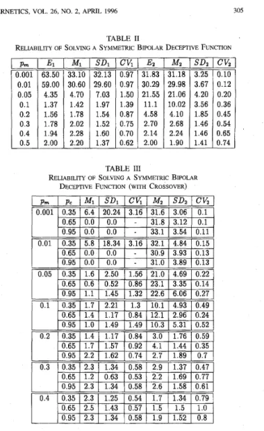
Using the mutation rates 0.001, 0.01, 0.05, 0.1, 0.2, 0.3, 0.4, 0.5, 0.6, 0.7, 0.8, 0.9, 0.95, 0.99, and 0.999, we computed the transition matrix Tpm in (29) and (30). Fig. 1 shows the compkation results of the deterministic model stated in Section V-A.

The horizontal axis identifies the mutation rate and the vertical axis indicates the occurrence ratio of optima in the final population (after 100 generations). Clearly, the curves are symmetrical with respect to p , = 0.5. This is because the transition matrices are symmetrical with respect to pn = 0.5 and both the occurrence vector 0' and the function vector F are symmetrical. Note that the upper bound of the occurrence ratio of optima is 50% when using disruptive selection. This upper bound is reasonable, since disruptive selection favors extreme (both superior and inferior) individuals.

It can be seen that in the range of 0.05-0.95 the proposed method has a larger occurrence ratio of optima than directional selection has. In contrast, in the ranges of [0.001 0.051 and [0.95 0.9991, the proposed method has a smaller occurrence ratio of optima. However,

IEEE TRANSACTIONS ON SYSTEMS, MAN, AND CYBERNETICS-PART B: CYBERNETICS, VOL. 26, NO. 2, APRIL 1996 29.98 21.06 10.02 4.10 2.68 2.24 1.90 305 3.67 4.20 3.56 1.85 1.46 1.46 1.41 Directional Selection 0.7 0.6 r pm p c m1 0.35 0.65 0.03. 0.35 0.65 0.95

o.ll

0.0 I

pB;*

I

,

,001 .01 .05 .1 .2 .3 .4 .5 .6 .7 .8 .9 .95 .99 ,999 MI SDI CV, M2 SD2 CV, 6.4 20.24 3.16 31.6 3.06 0.1 0.0 0.0 - 31.8 3.12 0.1 5.8 18.34 3.16 32.1 4.84 0.15 0.0 0.0 - 30.9 3.93 0.13 0.0 0.0 - 33.1 3.54 0.11 Mutation Rates

Convergence of solving A symmetric bipolar deceptive function Fig. 1. 0.05 0.6 0.5 R 0.4 a 0.3 O 0.1 Disruptive Selection

t

0.2 0.0 I I I I I I I I I I 0 5 10 15 20 25 30 35 40 45 50 55 60 65 0.95 0.0 0.0 - 31.0 3.89 0.13 0.35 1.6 2.50 1.56 21.0 4.69 0.22 0.65 0.6 0.52 0.86 23.1 3.35 0.14 Generations

Fig. 2. Comparison of rapidity on solving A symmetric bipolar deceptive function. 0.1 0.2 0.3 - 0.4 computing the occurrence ratio of optima through the deterministic

model, we observe that GA’s using the proposed method find the optima more quickly than GA’s using the conventional method. This observation is depicted (for p m = 0.01) in Fig. 2.

Here, the horizontal axis indicates the number of generations. Clearly, in the early generations, GA’s using disruptive selection have a higher Occurrence ratio of optima than GA’s using directional selection.

Since (29) and (30) involve probability, there is an intrinsic difference between experimental results obtained by actually applying GA’s and computation results obtained via these equations. It is reasonable to believe 1 hat a higher occurrence ratio of optima in the early stages implies greater reliability of the ratio in the final result. To verify this conjecture, we conducted several experiments using the following paramefers:

Population size: 64

Initial population: randomized Generations: 100

Mutation rates: 0.001, 0.01, 0.05, 0.1, 0.2, 0.3, 0.4, and 0.5. Each application of a GA consisted of 50 reinitialized runs. After replicating 50 runs, we computed the mean number of instances of the optima in the final population and the variation of the observed values. Table I1 presents the experimental results; here

E is the expected number of instances of the optima

A4 is the mean number of instances of the optima

S D is the standard deviation of the 50 numbers of instances of the optima

C V is the coefficient of variation, defined as S D I M .

A subscript 1 signifies directional selection and 2 disruptive

0.95 1.1 1.45 1.32 22.6 6.06 0.27 0.35 1.7 2.21 1.3 10.1 4.93 0.49 0.65 1.4 1.17 0.84 12.1 2.96 0.24 0.95 1.0 1.49 1.49 10.3 5.31 0.52 0.35 1.4 1.17 0.84 3.0 1.76 0.59 0.65 1.7 1.57 0.92 4.1 1.44 0.35 0.95 2.2 1.62 0.74 2.7 1.89 0.7 0.35 2.3 1.34 0.58 2.9 1.37 0.47 0.65 1.2 0.63 0.53 2.2 1.69 0.77 0.95 2.3 1.34 0.58 2.6 1.58 0.61 0.35 2.3 1.25 0.54 1.7 1.34 0.79 0.65 2.5 1.43 0.57 1.5 1.5 1.0 0.95 2.3 1.34 0.58 1.9 1.52 0.8 TABLE I1

RELIABILITY OF SOLVING A SYMMETRIC BIPOLAR DECEPTIVE FUNCTION

0.01 0.05 0.1 0.2 0.3 0.4 0.5 59.00 4.35 1.37 1.!56 1.’78 1 .!34 2.00 - Mi 33.10 30.60 4.70 1.42 1.78 2.02 2.28 2.20 __

-

SDI 32.13 29.60

1

7.03 1.97 1.54 1.52 1.60 1.37

-

-

Cv, 0.97 0.97 1.50 1.39 0.87 0.75 0.70 0.62

-

-

~

&

__ 31.83 30.29 1 21.55 11.1 4.58 2.70 2.14 2.00 TABLE I11

RELIABILITY OF SOLVING A SYMMETRIC BIPOLAR DECEPTIVE FUNCTION (WITH CROSSOVER)

~ __ 0.10 0.12 0.20 0.36 0.45 0.54 0.65 0.74

Obviously, directional selection usually resulted in a higher varia- tion than disruptive selection did. This result verifies our conjecture; an early, slight deviation from the computation value eventually leads to a great divergence from the expected result. This effect was clear in solving such a deceptive function, since the deceptive attractors are the second-best solution and are in the majority. Note that, for p m = 0.5, the behavior of a GA is just like a random search. Thus,

a contrary result is not surprising.

Since it is well known that the power of GA’s does not come from selection and mutation only, we also conducted experiments including the crossover operator to support our argument. Here, we replicated ten runs for each combination of parameter settings. Table I11 presents the results. It can be seen that disruptive selection is clearly superior to directional selection in solving this type of deceptive problem. From Tables I1 and I11 we can see that the crossover operator does not provide benefits when disruptive selection is used and it brings drawbacks when directional selection is used. This could be because the test function is deceptive for which GA’s are prone to be trapped at a deceptive local optimum, thus the crossover operator plays a negative role.

C. Why Disruptive Selection Works

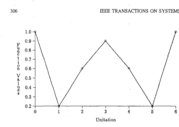
To explain why disruptive selection works, we characterize the deceptive function by its landscape. Fig. 3 shows the landscape of a

306 E E E TRANSACTIONS ON SYSTEMS, MAN, AND CYBERNETICS-PART B: CYBERNETICS, VOL. 26, NO. 2, APRIL 1996

1.0 4 ?

0.001

y

0.4 Unitation

Landscape of a symmetric bipolar deceptive function in unitation Fig. 3.

space.

TABLE IV

PROBABILITY OF BEING MUTATED m o THE GLOBAL OPTIMA

-

P777 0.001 0.01 0.05 0.1 0.2 0.3 0.4 0.5 - - ut=O ( u t = l j u t = 2 0.735 0.039 0.002 0.531 0.059 0.007 0.262 0.066 0.017 0.118 0.052 0.026 0.052 0.037 0.030 0.031 0.031 0.031 ut = 3 0.0 0.0 0.0 0.0 0.004 0.009 0.014 0.031 u t = 4 0.0 0.0 0.002 0.007 0.017 0.026 0.030 0.031

It is easy to see that the global optima are

u t = 5 ( u t = 6 0.001 0.994 0.01 0.941 0.039 0.735 0.059 0.531 0.066 0.262 0.052 0.118 0.037 0.052

I

0.031 0.031 surrounded (in a Hamming sense) by worst solutions and that the local optima (strings with unitation ut = 3) are surrounded by better solutions (strings with unitation ut = 2 or ut

=

4). These features imply that worst solutions, those with either unitation ut = 1 or ut = 5, have a greater chance of being mutated into optimal solutions and that better solutions are prone to be mutated into local optima. To ascertain whether this implication is true, we used (20) to compute the probability a string has to be mutated into the global optima (strings

000000 and 111 111) and the local optima (strings with unkation

ut = 3) under the mutation rate p m . Tables

IV

and V show the computation results from (20). These results confirm the implication. From Tables IV and V, we observe one common feature of these data, namely, there are two types of attractors, global optima and local optima, in the landscape. The force of attraction is dependent on the Hamming distance between one point and the attractor. The nearer a point is to an attractor, the stronger the force of attraction is. This feature explains why traditional GA’s are sometimes misled to deceptive attractors and why disruptive GA’s perform well.

VI. DISCUSSION AND CONCLUSIONS

Since all traditional GA’s use a monotonic fitness function and apply the “survival-of-the-fittest” principle to reproduce the new population, they can be viewed as a process of evolution that is based on directional selection. In this paper, we have proposed a type of disruptive selection that uses a nonmonotonic fitness function. The major difference between disruptive selection and directional selection is that the new method devotes more trials to both better solutions and worse solutions than it does to moderate solutions, whereas the traditional method allocates its attention according to the performance of each individual.

The experimental results reported here show that GA’s using the proposed method easily find the optimum of a function that is

nondeceptive but GA-hard. Since the sampling error is inevitable,

TABLE V

PROBASILrN OF BEING MUTATED INTO THE LOCAL OPTIMA u t = O I ? I t = l j u t = Z I u t = 3 0.038 0.156 0.245 0.312 0.320 0.315 0.313 u t = 5 I u t = 6 0.002

traditional GA’s do not perform well with functions that have large variance within schemata. However, using disruptive selection, a GA implicitly allocate more trials to schemata that have a large deviation from the mean value of a population. This statistic provides a good estimate of the real variance of the schema. Experimental results also show that GA’s using disruptive selection find the optima of a deceptive function more quickly and reliably than GA’s using directional selection do. This could be because the global optima of a deceptive function are surrounded by the worst solutions and the local optima are surrounded by better solutions. Since disruptwe selection also favors inferior individuals, GA’s using disruptive selection are immune to traps. Although we have tested this method on only two such functions, it might be applied successfully to other kinds of problems. Since disruptive selection favors both superior and inferior individuals, GA’s using disruptive selection will very likely perform well on problems easily solved by traditional GA’s. If GA’s using disruptive selection should not work well on them, we can implement a parallel GA in which disruptive selection and directional selection are used in different nodes and migration of good solutions occurs between different nodes periodically. Thus, as a supplement to directional selection, disruptive selection promises to be helpful in solving problems that are hard to optimize using traditional GA’s.

ACKNOWLEDGMENT

The authors would like to thank the three anonymous reviewers and the editor for their valuable suggestions for improving this paper.

REFERENCES

[l] D. H . Ackley, A Connectionist Machine for Genetic Hillclimbing. Boston, MA: Kluwer, 1987.

[2] J. E. Baker, “Adaptive selection methods for genetic algorithms,” in Proc. First Int. Con$ on Genetic Algorithms and Their Applications. Hillsdale, NJ Lawrence Erlbaum, 1985, pp. 101-111.

[3] -, “Reducing bias and inefficiency in the selection algorithm,” in Proc. Second Int. Con$ on Genetic Algorithms and Their Application. Hillsdale, NJ: Lawrence Erlbaum, 1987, pp. 1421.

[4] B. Bhanu, S. Lee, and J. Ming, “Self-optimizing image segmentation system using a genetic algorithm,” in Proc. Fourth Int. Con$ on Genetic Algorithms. San Mateo, CA: Morgan Kaufmann, 1991, pp. 362-369. [5] G. A. Cleveland and S. F. Smith, “Using .genetic algorithms to schedule

flow shop releases,” in Proc. Third Int. Con$ on Genetic Algorithms. San Mateo, CA: Morgan Kaufmann, 1989, pp. 160-169.

[6] K. Deb, J. Horn, and D. E. Goldberg, “Multimodal deceptive functions,” Univ. of Illinois at Urbana-Champaign, IlliGAL Report no. 92003, 1992. [7] K. A. DeJong, “An analysis of the behavior of a class of genetic adaptive

systems,” Ph.D. dissertation, Univ. Mich., Ann Arbor, MI, 1975. [8] -, “Learning with genetic algorithms: An overview,” Machine

Learning, vol. 3, pp. 121-138, 1988.

[9] M. Dorigo and U. Schnepf, “Genetic-based machine learning and behavior-based robotics: A new synthesis,” IEEE Trans. Syst., Man, Cybern., vol. 23, no. 1, pp. 141-154, 1993.

[IO] L. J. Eshelman, R. A. Caruana, and J. D. Schaffer, “Biases in the crossover landscape,” in Proc. Third Int. Con$ on Genetic Algorithms. San Mateo, CA, Morgan Kaufmann, 1989, pp. 10-19.

IEEE TRANSACTIONS ON SYSTEMS, MAN, AND CYBERNETICS-PART B: CYBERNETICS, VOL. 261, NO. 2, APRIL 1996 307

[ l 11 D. E. Goldberg and R. Lingle, Jr., “Alleles, loci, and traveling salesman problem,” in Proc. First Int. Con$ on Genetic Algorithms and Their Applications. Hillsd,de, NJ: Lawrence Erlbaum, 1985, pp. 154-159. [12] D. E. Goldberg, Genetic Algorithms in Search, Optimization and Ma-

chine Learning.

[13] D. E. Goldberg and K. Deb, “A comparative analysis of selection schemes used in genetic algorithms,” in Foundations of Genetic Al- gorithms, G. J. E. Rawlins, Ed. San Mateo, C A Morgan Kaufmann, 1991, pp. 69-93.

[14] J. J. Grefenstette, R. Gopal, B. Rosmaita, and D. V. Gucht, “Genetic algorithms for the traveling salesman problem,” in Proc. First Int. Con$ on Genetic Algorithms and Their Applications. Hillsdale, NJ: Lawrence Erlbaum, 1985, pp. 160-168.

[I51 J. J. Grefenstette, “Optimization of control parameters for genetic algorithms,” IEEE Trams. Syst., Man, Cybem., vol. SMC-16, no. 1, pp. 122-128, 1986.

[16] -, “Credit assignment in rule discovery systems based on genetic algorithms,” Machine Learning, vol. 3 , pp. 225-245, 1988.

[17] J. J. Grefenstette and J. E. Baker, “How genetic algorithms work A critical look at implicit parallelism,” in Proc. Third Int. Con$ on Genetic Algorithms.

[IS] J. J. Grefenstette, “Deception considered harmful,” in Foundations of Genetic Algorithms 2, D. Whitley, Ed. San Mateo, CA: Morgan Kaufmann, 1992, pp 75-91.

[19] S. A. Harp, T. Samad, and A. Guha, “Towards the genetic synthesis of neural networks,” in Proc. Third Int. Con$ on Genetic Algorithms. San Mateo, CA: Morgan Kaufmann, 1989, pp. 360-369.

[20] J. H. Holland, Adaptation in Natural and Artijicial Systems. Ann Arbor, MI: Univ. Mich. Press, 1975.

[21] __, “Searching nonlinear functions for high values,” Appl. Math. Comp., vol. 32, pp. 255-274, 1989.

[22] C. L. Karr, “Design of an adaptive fuzzy logic controller using a genetic algorithm,” in Proc. Fourth Int. Con$ on Genetic Algorithms.. San Mateo, CA: Morgan Kaufmann, 1991, pp. 450457.

[23] K. Kristinsson and C. A. Dumont, “System identification and control using genetic algorithms,” IEEE Trans. Syst., Man, and Cybern., vol. 22, no. 5 , pp. 1033-1046, 1992.

[24] T. Kuo and S. Y. Hwang, “A genetic algorithm with disruptive selec- tion,” in Proc. Fifth Imt. Con$ on Genetic Algorithms. San Mateo, CA: Morgan Kaufmann, 1993, pp. 65-69.

[25] G. E. Liepins and M. D. Vose, “Deceptiveness and genetic algorithm dynamics,” in Found,ztions of Genetic Algorithms, G. J. E. Rawlins, Ed. San Mateo, CA: Mo-gan Kaufmann, 1991, pp. 36-50.

[26] B. F. J. Manly, The Statistics of Natural Selection on Animal Popula- tions. London, UK Chapman and Hall, 1984.

[27] G. F. Miller, P. M. Todd, and S. U. Hegde, “Designing neural net- works using genetic algorithms,” in Proc. Third Int. Con5 on Genetic Algorithms. San Mateo, CA, Morgan Kaufmann, 1989, pp. 379-384. [28] J. D. Schaffer and A. Morishima, “An adaptive crossover distribution

mechanism for genetic algorithms,” in Proc. Second Int. Con$ on Genetic Algorithms und Their Applications. Hillsdale, NJ: Lawrence Erlbaum Associates, 1987, pp. 36-40.

[29] G. Syswerda, “Uniform crossover in genetic algorithms,” in Proc. Third Int. Con$ on Genetic Algorithms. San Mateo, CA: Morgan Kaufmann, 1989, pp. 2-9.

[30] G. Syswerda and J. I’almucci, “The application of genetic algorithms to resource scheduling,” in Proc. Fourth Int. ConJ on Genetic Algorithms. San Mateo, CA: Morgan Kaufmann, 1991, pp. 502-508.

[31] D. Whitley and J. K.auth, “GENITOR. a different genetic algorithm,” in Proc. Rocky Mountain Con$ on Art$cial Intelligence, 1988, pp. 118-130.

[32] D. Whitley, “Fundaniental principles of deception in genetic search,” in Foundations of Genetic Algorithms, G. J. E. Rawlins, Ed. San Mateo, CA: Morgan Kaufm.mn, 1991, pp. 221-241.

[33] S. W. Wilson, “GA-easy does not imply steepest-ascent optimizable,” in Proc. Fourth Int. Cor$ on Genetic Algorithms. San Mateo, CA: Morgan Kaufmann, 1991, pp. 85-89.

Restding, MA: Addison-Wesley, 1989.

San Mateo, CA: Morgan Kaufmann, 1989, pp. 20-27.

A Constructive Approach for Nonlinear System

Identification Using Multilayer Perceptrons

Ju-Yeop Choi, Hugh F. VanLandingham, and Stanoje Bingulac

Abstract-This paper combines a conventional method of multivariable system identification with a dynamic multi-layer perceptron (MLP) to achieve a constructive method of nonlinear system identification. The class of nonlinear systems is assumed to operate nominally around an equilibrium point in the neighborhood of which a linearized model exists to represent the system, although normal operation is not limited to the linear region. The result is an accurate discrete-time nonlinear model, extended from a MIMO linear model, which captures the nonlinear behavior of the system.

I. INTRODUCTION

Since real-world systems resist being modeled in precise math- ematical terms due to unknown dynamics and, typically, a noisy environment, it is very difficult to determine an exact model for a complex nonlinear system. Consequently, there is a need for a nonclassical technique which has the ability to accurately model these physical processes. It has been shown that multi-layer perceptrons (MLP’s), one of the many forms of artificial neural networks (ANN’S) is a universal l’unction approximator, i.e., with sufficient training on appropriate inpat/output data, MLP’s can represent arbitrarily closely any smooth vector map [l], [2]. Although the theory of linear system identification may now be considered to be a mature discipline, new techniques, particularly for nonlinear system identification, continue to be of interest. In this paper such a method is addressed in the context of using neural networks [3], [4]. Neural networks of various types and structures (paradigms) have been found to be efficient tools for identifying nonlinear systems, e.g., through Volterra series models, GMDH models, SONN models and radial basis functions [5]-[8]. Among the researchers of the control community using ANN’S

over the past two decades, Narendra [9]-1111 has used dynamic ANN’S as components in dynamical systems, concentrating on system identification and control of nonlinear plants. Pao introduced the functional-link net which constructs a nonlinear mapping at the input layer to reduce the complexity of ANN’S [12]. Although there are many techniques available for the corresponding linear identification

problem, MLP’s may be regarded as a nonclassical technique which can accomplish similar results using only input/output data, i.e., without prior model information. Most importantly, MLP’s do not require the usual assumption of linearity. Thus, although it is true that neural networks can offer little, if any, improvement over existing methods of identification of linear systems, they do present a

potential for c,apturing the complex nonlinearities of a wide class of industrial processes in a universal manner never before imagined [13]. However, there are many difficult problems to overcome, such as when the nonlinear system is found to be both complex and unstable. This latter condition complicates the “training” of the MLP [14]. One approach is to stabilize the system locally. Such stabilization of a nonlinear dynamic system can be done for systems which are Manuscript received August 27, 1993; revised May 18, 1994, and December 28, 1995.

J.-Y. Choi and H. F. VanLandingham are with the Bradley Department of Electrical Engineering, Virginia Polytechnic Institute and State University,

Blacksburg, VA 24061-01 11 USA (e-mail: hughv@vt.edu).

S. Bingulac i:j with the Department of Electrical and Computer Engineering, Kuwait University, 13060 Safat, Kuwait.

Publisher Item Identifier S 1083-4419(96)02308-4.