Fractional Steps Scheme of Finite Analytic Method
for Advection–Diffusion Equation
Tung-Lin Tsai
1; Chung-Min Tseng
2; and Jinn-Chuang Yang
3Abstract: For simply finding local analytic solution, the time derivative in the traditional finite analytic (FA) method is generally
replaced with a first-order finite difference approximation as a source term. However, this may induce excessive numerical diffusion, especially for advection-dominated transport problems. In this paper, a fractional steps scheme of the FA method without using the finite difference approximation to time derivative is proposed by applying the one-dimensional FA method whose local analytic solution is obtained from both spatial and time domains, together with the method of fractional steps. Four hypothetical examples, including two-dimensional and three-dimensional cases, are employed to investigate this newly proposed method as compared with the traditional FA method, the optimal unsteady FA method, and the alternating direction scheme of the hybrid FA method. The results show that the fractional steps scheme of the FA method can greatly diminish numerical diffusion and is superior to the other methods compared herein. DOI:10.1061/(ASCE)0733-9399(2005)131:1(23)
CE Database subject headings:Analytical techniques; Finite differences; Diffusion.
Introduction
The finite analytic (FA) method, unlike the finite difference method which applies the Taylor series expansion formulation or the finite element method which uses the interpolation function and weighting function, was first proposed by Chen et al.(1981) and has been applied to many fields. Chen and Chen(1984), Chen et al.(1987), Aksoy and Chen (1992), and Chen et al. (1995), for example, used the FA method to compute Navier–Stokes equa-tions. The FA method was also employed not only to the sus-pended sediment transport in river channel by Fang and Wang (2000) but also to the solute transport in two-dimensional (2D) groundwater flow by Hwang et al.(1985), Tsai et al. (1995), and Tsai et al.(2000).
The FA method is based on finding an analytic solution to a linear or linearized differential equation on a small subdomain of problem domain. For the one-dimensional(1D) case, two types of local analytic solutions could be found. With specifying proper initial and boundary conditions in a subdomain and applying the method of separation of variables, the first type of the local ana-lytic solution is obtained by solving a partial differential equation. The second one is given by replacing the time derivative with a first-order finite difference approximation as a source term for
solving an ordinary differential equation. The major difference between these two types of local analytic solutions is that the former is found from both spatial and time domains, but the latter, namely the hybrid FA method, is only derived from spatial do-main. However, for 2D and three-dimensional (3D) cases, only hybrid formulation could be applied to the FA method due to the difficulty in finding local analytic solution from both spatial and time domains.
In the FA method, the use of the first-order finite difference approximation to time derivative may deteriorate the computa-tional results, especially for the large Péclect number. To tackle this problem, Tsai and Chen(1995) proposed an optimal unsteady FA method that introduced an optimal time-weighting factor to improve the approximation for the time derivative in the tradi-tional FA method. The optimal time-weighting factor is obtained from the analytic solution of 1D linear advection and diffusion of a sharp front concentration following a uniform flow velocity and a constant diffusion coefficient in an infinite domain. However, with the use of the optimal time-weighting factor, the simulating cost may increase, especially for 3D problems, due to the need for a predictor–corrector computational procedure. Alternatively, based on the use of the 1D hybrid FA method (only the local spatial analytic solution is found) and applying the alternating direction implicit method (Peaceman and Rachford 1955) to in-crease the accuracy of the approximation for time derivative, there is another kind of FA method, namely the alternating direc-tion scheme of the hybrid FA method(Lu et al. 1990; Lu and Shi 1990; Lu and Chen 1992; and Yang and Li 1992). In addition, in order to obviate the use of the finite difference approximation to the time derivative, Li et al.(1992) applied the Laplace transform technique to deal with the time derivative and obtained satisfac-tory results for the 1D solute transport equation. However, the application of the Laplace transformation is limited to linear dif-ferential equations and transposable boundary conditions. More-over, calculation of the corresponding inverse Laplace transfor-mation may be difficult, especially for multidimensional problems.
In this paper, a fractional steps scheme of the FA method
with-1Research Assistant Professor, Natural Hazard Mitigation Research
Center(NHMRC), National Chiao Tung Univ., Hsinchu, Taiwan 30010, R.O.C.
2
Section Chief, Water Resources Agency, Ministry of Economic Affairs, Taipei, Taiwan 106, R.O.C.
3Professor, Dept. of Civil Engineering and Research Fellow of
NHMRC, National Chiao Tung Univ., Hsinchu, Taiwan 30010, R.O.C. Note. Associate Editor: Henry K. Stolarski. Discussion open until June 1, 2005. Separate discussions must be submitted for individual pa-pers. To extend the closing date by one month, a written request must be filed with the ASCE Managing Editor. The manuscript for this paper was submitted for review and possible publication on February 20, 2003; approved on June 4, 2004. This paper is part of the Journal of
Engineer-ing Mechanics, Vol. 131, No. 1, January 1, 2005. ©ASCE, ISSN
0733-9399/2005/1-23–30/$25.00.
out using finite difference approximation to time derivative is proposed to solve the multidimensional advection–diffusion equa-tion by applying the method of fracequa-tional steps (Yanenko 1971; Tsai et al. 2001; Tsai et al. 2002), together with 1D FA method whose local analytic solution is found from both spatial and time domains. In order to examine this new type of FA method, four hypothetical examples, including 2D and 3D cases, are consid-ered. Comparisons of simulated results by the traditional FA method, the optimal unsteady FA method, the alternating direc-tion scheme of the hybrid FA method, and the present scheme are conducted.
Brief Reviews of Former Finite Analytic Methods Optimal Unsteady Finite Analytic Method
The 2D advection–diffusion equation can be written as ⌽ t + u ⌽ x +v ⌽ y =x 2⌽ x2+y 2⌽ y2 共1兲
where ⌽⫽concentration of contaminant or temperature; x and
y⫽spatial coordinates; t⫽time; u andv⫽velocity components of flow in x and y directions, respectively; andxandy⫽diffusion
coefficients. In Eq. (1), u, v,x, andy may be given as
func-tions of x , y, and t.
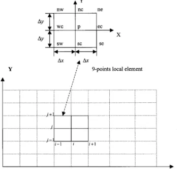
In the FA method, the solution domain is subdivided into small element of 2⌬x by 2⌬y as shown in Fig. 1. ⌬x and ⌬y are grid sizes in x and y directions, respectively. Eq. (1) for each local element can be linearized and evaluated at time step n as
1 共x兲i,j n
冉
⌽ t冊
i,j n + 2A ⌽ n x + 2BC ⌽n y = 2⌽n x2 + C 2⌽n y2 共2兲 where A =共u兲i,jn /共2x兲i,jn ; B =共v兲 i,j n/共2 y兲i,j n; and C =共 x兲i,j n/共 y兲i,j n.
The superscript n represents values evaluated at the 共n兲th time step. The subscript共i, j兲 represents values evaluated at the central node of rectangular local element as shown in Fig. 1.
The ease in finding an analytic solution to Eq. (2) is greatly increased greatly by replacing the time derivative with a finite difference approximation as
冉
⌽ t冊
i,j n = 1 1 −冋
⌽i,j n −⌽ i,j n−1 ⌬t −冉
⌽ t冊
i,j n−1册
共3兲where⫽time-weighting factor and ⌬t⫽time step. In the tradi-tional FA method, the time-weighting factor is equal to zero共 = 0兲, that is, a first-order finite difference approximation for time derivative. The optimal unsteady FA method (Tsai and Chen 1995) was presented with the introduction of an optimal time-weighting factor as = 0.5
冤
冉
⌽ t冊
i,j n−1 ⌽i,j n −⌽ i,j n−1 ⌬t冥
−0.28 共4兲Substituting Eq. (3) into Eq. (2) and specifying four boundary conditions for a local element as shown in Fig. 1, an analytic solution to Eq.(2) could be found in each local element using the method of separation of variables. When this local analytic solu-tion is evaluated at the central node共i, j兲 of the local element, an algebraic equation relating the evaluated nodal value to its eight neighboring nodal values and central nodal value at previous time step could be expressed as
冋
1 + aP 共1 − 兲⌬t共x兲i,jn册
⌽i,j n = a NW⌽i−1,j+1 n + a SE⌽i+1,j−1 n + aSW⌽i−1,j−1 n + aWC⌽i−1,j n + aEC⌽i+1,j n + aNC⌽i,j+1 n + a SC⌽i,j−1 n + a NE⌽i+1,j+1 n + ai,j ⌬t共1 − 兲共x兲i,jn ⌽i,j n−1 + 共1 − 兲共x兲i,j n冉
⌽ t冊
i,j n−1 共5兲 where the FA coefficients aP, aNW,…, aNEcould be obtained byChen and Chen(1984) and Hwang et al. (1985). Eq. (5) could be applied for each unknown nodal point to construct a set of alge-braic equations.
Alternating Direction Scheme of Hybrid Finite Analytic Method
The component of Eq.(1) in the x direction can be written as ⌽ t + u ⌽ x =x 2⌽ x2 共6兲
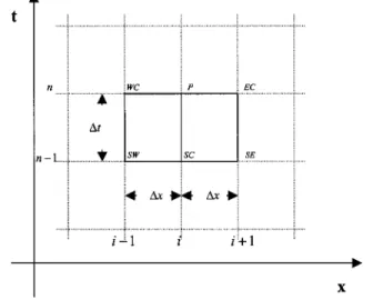
Like the traditional FA method as mentioned above, with the ap-plication of the first-order finite difference approximation to time derivative, Eq. (6) for a small element on both spatial and time domains as shown in Fig. 2 can be linearized and evaluated at time step n as
2⌽n
x2 = 2A1 ⌽n
x + s 共7兲
where A1=共u兲in/共2x兲in, and s =共⌽in−⌽in−1兲/共x兲in⌬t.
Fig. 1.Nine-points local element for two-dimensional finite analytic method
Eq.(7) is a linear ordinary differential equation that could be easily solved. With the local analytic solution, the FA algebraic equation at central point i in a local element as shown in Fig. 2 could be expressed as ⌽in−⌽i n−1 ⌬t = 共u兲in 2⌬x sinh共A1⌬x兲共e A1⌬x⌽ i−1 n − 2 cosh共A1⌬x兲⌽ i n + e−A1⌬x⌽ i+1 n 兲 共8兲
Eq.(8) is the so-called 1D hybrid FA method whose local analytic solution is only found from spatial domain as shown in Eq.(7).
Applying the idea of the alternating direction implicit method (Peaceman and Rachford 1955) together with the 1D hybrid FA method as shown in Eq. (8), an alternating direction scheme of the hybrid FA method has been proposed to solve the 2D advection–diffusion equation as follows:
⌽i,,j n−1/2 −⌽i,j n−1 ⌬t/2 = Lx⌽i,j n−1/2+ L y⌽i,j n−1 共9兲 ⌽i,,j n −⌽i,j n−1/2 ⌬t/2 = Lx⌽i,j n−1/2+ L y⌽i,j n 共10兲 in which Lx⌽i,j= 共u兲i,j n 2⌬x sinh共A1*⌬x兲共e A1*⌬x⌽
i−1,j− 2 cosh共A1*⌬x兲⌽i,j
+ e−A1 *⌬x
⌽i,j兲 共11兲
Ly⌽i,j=
共v兲i,jn 2⌬y sinh共B1*⌬x兲共e
B1*⌬y⌽
i,j−1− 2 cosh共B1*⌬y兲⌽i,j
+ e−B1*⌬x⌽
i,j+1兲 共12兲
where A1*=共u兲i,jn/共2x兲i,j n; and B 1 *=共v兲 i,j n/共2 y兲i,j n.
Fractional Steps Scheme of Finite Analytic Method The traditional FA method, the optimal unsteady FA method, and the alternating direction scheme of the hybrid FA method, as men-tioned above, are all developed based on the use of the finite difference approximation to time derivative. However, in the
dif-ferent types of FA methods, only 1D FA method (not including the 1D hybrid FA method) does not need the use of the finite difference approximation to time derivative, and then obtains the local analytic solution from both time and spatial domains(Chen and Chen 1982). The 1D FA method could be straightforwardly applied to solve multidimensional problems in conjunction with the method of fractional steps (Yanenko 1971; Tsai et al. 2001, 2002)
Using the method of fractional steps, the 2D advection– diffusion equation as shown in Eq. (1) can be decoupled into a series of 1D advection–diffusion equations as
⌽ t + u ⌽ x =x 2⌽ x2 共13兲 and ⌽ t +v ⌽ y =y 2⌽ y2 共14兲
By approximating the flow velocity and diffusion coefficient as a constant over a small element as shown in Fig. 2, the linerized 1D advection–diffusion equation as shown in Eq. (13) can be ex-pressed as B2 ⌽ t + 2A2 ⌽ x = 2⌽ x2 共15兲 where A2=共u兲i n/共2 x兲i nand B 2= 1 /共x兲i n.
Eq. (15) can be solved analytically in a small element by the method of separation of variables with the initial and boundary conditions are specified as
⌽共x,0兲 = as共e2A2x− 1兲 + bsx + cs 共16兲
⌽共− ⌬x,t兲 = aw+ bwt 共17兲
⌽共⌬x,t兲 = aE+ bEt 共18兲
where the node i is taken as the origin. The coefficients in Eqs. (16)–(18) could be found in terms of the nodal values at the element boundaries as shown in Fig. 2
Evaluating the analytic solution for nodal point i an algebraic equation giving the nodal value⌽inas a function of its five neigh-boring nodal values shown in Fig. 2 can be expressed as
⌽in= bWC⌽i−1n + bEC⌽i+1n + bSW⌽i−1n−1+ bSE⌽i+1n−1+ bSC⌽in−1
共19兲 where the coefficients bWC, bEC, bSW, aSE, and bSC in Eq. (19)
are functions of A2, B2,⌬x, and ⌬t (Chen and Chen 1982) and are displayed in the Appendix. Eq.(19) is a 1D FA method whose local analytic solution is found from both time and spatial do-mains with the partial differential equation as given in Eq. (15) and initial and boundary conditions as shown in Eqs.(16)–(18).
The 1D FA method, i.e., Eq.(19), can be rewritten as
Ax⌽in= Bx⌽in−1 共20兲
with introducing operators Axand Bxas
Ax⌽i= − bWC⌽i−1+⌽i− bEC⌽i+1 共21兲
and
Fig. 2.Local element in one-dimensional finite analytic method
Bx⌽i= bSW⌽i−1+ bSC⌽i+ bSE⌽i+1 共22兲
Thus, based on the technique of the fractional steps scheme as shown in Eqs.(13) and (14), together with the 1D FA method as shown in Eq. (21) for the x component and the one for the y component that can be easily found based on Eq.(20), a fractional steps scheme of the FA method is proposed to solve the 2D advection–diffusion equation as follows:
Ax⌽i,j * = Bx⌽i,j n−1 共23兲 Ay⌽i,jn = By⌽i,j* 共24兲 Here
Ax⌽i,j= − bWC⌽i−1,j+⌽i,j− bEC⌽i+1,j
共25兲
Bx⌽i,j= bSW⌽i−1,j+ bSC⌽i,j+ bSE⌽i+1,j
and
Ay⌽i,j= − bWC⌽i,j−1+⌽i,j− bEC⌽i,j+1
共26兲
By⌽i,j= bSW⌽i,j−1+ bSC⌽i,j+ bSE⌽i,j+1
where the superscript ⴱ denotes intermediate value. The coeffi-cients bWC, bEC, bSW, bSE, and bSCin Eq. (25) can be evaluated
as shown in Eq. (19) with A2=共u兲i,jn/共2x兲i,j n; and B
2= 1 /共x兲i,j n;
Similarly, the coefficients bWC, bEC, bSW, bSE, and bSC in Eq.
(26) can be calculated as given in Eq. (19) with A2 =共v兲i,jn /共2y兲i,j
n; B
2= 1 /共y兲i,j
n; and replacing⌬x by ⌬y. The sketch
of computational procedure for the fractional steps scheme of the FA method is depicted in Fig. 3.
Demonstrations and Evaluations
Advection and Diffusion of Point Source Contaminant In order to examine the performances of the fractional steps scheme of the FA method, the advection and diffusion of a point source contaminant in a uniform flow is considered first. The problem is given by ⌽ t + U ⌽ x =x 2⌽ x2+y 2⌽ y2 共27兲
with boundary conditions of
⌽共x,y,t兲 → 0 as 兩x兩 → ± ⬁ or 兩y兩 → ± ⬁ 共28兲 where U⫽constant flow velocity in the x direction. When the initial condition is a point source of mass M at x = x0and y = y0, the well-known exact solution is
⌽共x,y,t兲 = M 4t共xy兲1/2 exp
再
−关共x − x0兲 − Ut兴 2 4xt −共y − y0兲 2 4yt冎
共29兲 To allow a numerical solution based on an initial peak concentra-tion of unity, calculaconcentra-tion begins at time t = t0having a concentra-tion distribuconcentra-tion given by Eq.(29) with the point source of massM = 4t共xy兲1/2t0. In this numerical simulation, the following pa-rameters are used: t0= 1,000 s ; U = 2 m / s ;x= 3.2 m2/ s ;
y
= 1.6 m2/ s ; ⌬x=⌬y=40 m; ⌬t=15 s; and 共x0, y0兲 =共80 m,2,000 m兲.
Fig. 4 shows the contour plots of simulated results at time t =共t0+ 600兲 s by the fractional steps scheme of FA (FSSFA)
method, the alternating direction scheme of hybrid FA(ADSHFA) method, the optimal unsteady FA method, the traditional FA method, and the analytical solution. The computed results from those methods compared herein along the line y = 2,000 m are displayed in Fig. 5. From Figs. 4 and 5, one can clearly find that the traditional FA method induces larger numerical diffusion than the optimal unsteady FA method in which an optimal time-weighting factor is introduced. The computational result by the alternating direction scheme of the hybrid FA method seems to agree with the one yielded by the optimal unsteady FA method. The fractional steps scheme of the FA method can greatly de-crease numerical diffusion in comparison with the other three methods by evading the use of finite difference approximation to time derivative.
Advection and Diffusion of Line Source Contaminant This example simulates advection and diffusion of a line source contaminant in a uniform flow on semi-infinite domain as shown in Fig. 6. The governing equation is given by Eq.(27) with the boundary and initial conditions as follows:
⌽共0,y,t兲 = 1
共30兲 0艋 y 艋 y0
Fig. 3. Sketch of computational procedure for fractional steps scheme of finite analytic method
⌽共0,y,t兲 = 0 共31兲 y0艋 y 艋 y1 ⌽共⬁,y,t兲 = bounded 0艋 y 艋 y1 共32兲
冏
⌽ y冏
y=0 = 0 共33兲 x⬎ 0冏
⌽ y冏
y=y1 = 0 共34兲 x⬎ 0 ⌽共x,y,0兲 = 0 x⬎ 0 共35兲 0艋 y 艋 y1The exact solution was presented by Bruch and Street(1967). The FSSFA method, the ADSHFA method, the unsteady FA method, and the traditional FA method are used to simulate this problem. With y1= 20 m ; y0= 10 m ; U = 0.1 m / s ; ⌬x=⌬y=0.5 m; ⌬t = 4 s ; x= 0.003 m2/ s; andy= 0.001 m2/ s, the simulated results
at t = 80 s and on the line y = 5 m are displayed in Fig. 7. It is clearly found that the fractional steps scheme of the FA method has the best results in comparison with the other three schemes. The traditional FA method produces larger numerical diffusion among those methods compared herein. The simulated results by the alternating direction scheme of the hybrid FA solution and the optimal unsteady FA method are comparable.
Two-Dimensional Convective Transport Equation A 2D nondimensional convective transport equation with a uni-form flow is considered. The governing equation is
Fig. 4.Comparison of various schemes for advection and diffusion of point source contaminant:(a) traditional finite analytic method; (b) optimal unsteady finite analytic method; (c) alternating direction
scheme of hybrid finite analytic method;(d) fractional steps scheme of finite analytic method; and(e) exact solution
Fig. 5.Comparison of various schemes for advection and diffusion of point source contaminant(along line y =2,000 m)
Fig. 6.Domain and boundary conditions for calculation of advection and diffusion of line source contaminant
⌽ t + ⌽ x + ⌽ y = D
冉
2⌽ x2+ 2⌽ y2冊
共36兲where D represents the inverse of the Reynolds number. Under the initial condition
⌽共x,y,0兲 = sin共x兲 + sin共y兲 共37兲 and boundary conditions
⌽共0,y,t兲 = 共sin共− t兲 + sin 共y − t兲兲exp共− D2t兲 ⌽共1,y,t兲 = 共sin 共1 − t兲 + sin 共y − t兲兲exp共− D2t兲
⌽共x,0,t兲 = 共sin 共x − t兲 + sin共− t兲兲exp共− D2t兲
⌽共x,1,t兲 = 共sin 共x − t兲 + sin 共1 − t兲兲exp共− D2t兲 共38兲 the exact solution to Eq.(36) can be expressed as
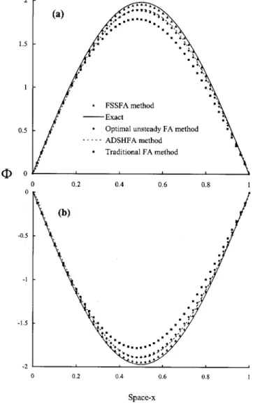
⌽共x,y,t兲 = 共sin 共x − t兲 + sin 共y − t兲兲exp共− D2t兲 共39兲 A uniform grid size of 0.02⫻0.02, time step of 0.025, and D = 0.0005 are used for this simulation. The computed results along the line y = x by the FSSFA method, the ADSHFA method, the optimal unsteady FA method, and the traditional FA method are displayed in Fig. 8. The results show that the traditional FA method induces severe numerical diffusion. The alternating direc-tion scheme of the FA method and the optimal unsteady FA method seem to provide comparable simulated results. The frac-tional steps scheme of the FA method, again, has the best results among the four methods considered.
Three-Dimensional Diffusion in Shear Flow
In order to further investigate the capability of the fractional steps scheme of the FA method, a case for 3D diffusion in a shear flow is studied. The velocity shear in the diffusion of a patch of passive contaminant from an instantaneous source plays an important role in groundwater flow or natural streams such as oceans, lakes, and estuaries. The governing equation for shear diffusion can be writ-ten as ⌽ t +共V0+⍀yy +⍀zz兲 ⌽ x = Dx 2⌽ x2+ Dy 2⌽ y2+ Dz 2⌽ z2 共40兲 where V0⫽mean velocity in the x direction; ⍀y and⍀z denote
horizontal and vertical shear, respectively; and Dx, Dy, and Dz
represent eddy diffusivities in x , y, and z directions, respectively. The analytical solution for an instantaneous point source of mass
M released at x = y = z = 0 was obtained by Carter and Okubo
(1965) as follows: ⌽共x,y,z,t兲 = M 83/2共D xDyDz兲1/2t3/2共1 + 2t2兲1/2 ⫻exp −
冋
共x − V0t − 0.5共⍀yy +⍀zz兲t兲2 4Dxt共1 + 2t2兲 + y 2 4Dyt + z 2 4Dzt册
共41兲 whereFig. 7.Comparison of various schemes for advection and diffusion of line source contaminant(along line y =8 m)
Fig. 8.Comparison of various schemes for the two-dimensional non-dimensional convective transport equation:(a) t=2 and (b) t=3
2=
b
共⍀y 2D y/Dx兲 + 共⍀z 2D z/Dx兲c
12 共42兲Allowing numerical solution to have an initial peak concentration of unity, simulation begins at time t = t0with the point source of mass M as
M = 83/2共D
xDyDz兲1/2t3/2共1 + 2t0
2兲1/2 共43兲 In the numerical simulation, t0= 1,000 s ; V0= 0.2 m / s ; ⍀y=⍀z
= 0.0002 1 / s ; Dx= Dy= Dz= 5.0 m2/ s ; ⌬t=100 s; and grid space
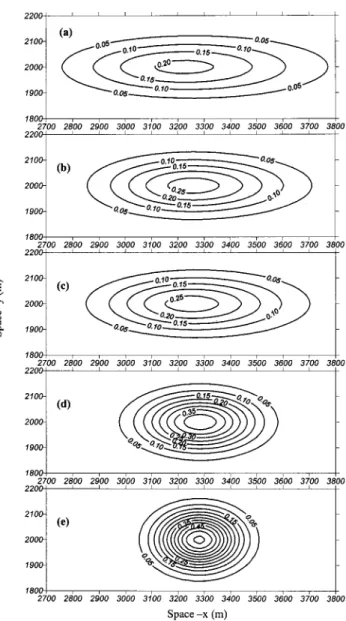
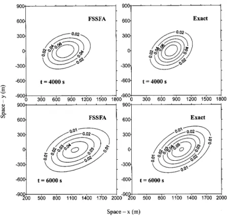
⌬x=⌬y=⌬z=100 m are used. Fig. 9 shows the contour plots of the fractional steps scheme of the FA method and the exact solu-tion at t = 4,000 and 6,000 s on the plane z = 0, respectively. From Fig. 9, one can observe that the fractional steps scheme of the FA method gives convincing simulated results.
Conclusions
The FA method, unlike the finite difference method which applies the Taylor series expansion formulation or the finite element method which uses the weighted residual method with interpola-tion funcinterpola-tion and weighting funcinterpola-tion, is based on finding an ana-lytic solution to a linear or linearized differential equation on a small subdomain of the problem domain. It is observed that re-placing the time derivative with a first-order finite difference ap-proximation in the traditional FA method may induce excessive numerical diffusion, especially for a large Péclect number. To improve the use of the first-order finite difference approximation to time derivative in the traditional FA method several alterna-tives, such as the applications of optimal time-weighting factor and the alternating direction implicit method, have been pre-sented. In this paper, a new fractional steps scheme of the FA method is proposed, in which the local analytic solution is found
from both time and spatial domains. It is as expected that the traditional FA method induces the largest numerical diffusion among the four methods compared herein. The alternating direc-tion scheme of the hybrid FA method and the optimal unsteady FA method seem to give comparably better results, while the pro-posed fractional steps scheme of the FA method gives the least numerical diffusion as compared with the other three methods due to avoiding the use of the finite difference approximation to the time derivative.
Appendix. Coefficients of One-Dimensional Finite Analytic Method bWC= eA2⌬xS1, 共44兲 bEC= e−A2⌬xS1 bSW= eA2⌬xS2, 共45兲 bSE= e−A2⌬xS2 bSC= 4A2⌬x cosh共A2⌬x兲coth共A2⌬x兲P2 共46兲 S1= B2⌬x2 ⌬t 共P2− Q2兲 + Q1 共47兲 S2= B2⌬x2 ⌬t 共Q2− P2兲 − 2A2⌬x coth共A2⌬x兲P2 共48兲 P2=
兺
m=1 ⬁ 共− 1兲m+1 m⌬xe−Fm⌬t 关共A2⌬x兲2+共 m⌬x兲2兴2 共49兲Fig. 9.Contour plots of diffusion in shear flow by fractional steps scheme of finite analytic on plane z = 0 at t = 4,000 and 6,000 s
Fm= A2 2 +m 2 B2 共50兲 m= 共2m − 1兲 2⌬x 共51兲 Q1= 1 eA2⌬x+ e−A2⌬x 共52兲 Q2= eA2⌬x− e−A2⌬x 2A2⌬x共eA2⌬x+ e−A2⌬x兲2 共53兲 Notation
The following symbols are used in this paper: D ⫽ the inverse of Reynolds number;
Dx, Dy, Dz ⫽ eddy diffusivities in x,y, and z directions;
Lx, Ly ⫽ operators;
u ,v, U ⫽ flow velocity component;
V0 ⫽ mean velocity in x direction; ⌬t ⫽ time increment;
⌬x,⌬y,⌬z ⫽ computational grid intervals in x, y, and z directions
x,y,z ⫽ diffusion coefficients in x, y, and z directions;
⌽ ⫽ concentration; and
⍀y,⍀z ⫽ horizontal and vertical shear.
Subscripts
i , j ⫽ x and y directional computational point index.
Superscripts
n ⫽ time step index.
References
Aksoy, H., and Chen, C. J.(1992). “Numerical solution of Navier-Stokes equations with nonstaggered grids using finite analytic method.” Numer. Heat Transfer, Part B, 21, 287–306.
Bruch, J. C., and Street, R. L.(1967). “Two-dimensional dispersion.” J. Sanit. Eng. Div., Am. Soc. Civ. Eng., 93(6), 17–39.
Cater, H. H., and Okubo, A.(1965). A study of the physical process of movement and dispersion in Cape Kennedy area. Final Rep. U.S. American Energy Communication Contract No. AT (30-1).
Chen, C. J., Bravo, R. H., Chen, H. C., and Xu, Z.(1995). “Accurate discretization of incompressible three-dimensional Navier-Stokes
equations.” Numer. Heat Transfer, Part B, 27, 371–392.
Chen, C. J., Naser-Neshat, H., and Ho, K. S. (1981). “Finite analytic numerical solution of heat transfer in two-dimensional cavity flow.” Numer. Heat Transfer, 4, 179–197.
Chen, C. J., Yu, C. H., and Chandran, K. B. (1987). “Finite analytic Numerical solution of unsteady laminar flow past disc-valves.” J. Eng. Mech., 113(8), 1147–1162.
Chen, H. C., and Chen, C. J.(1982). The finite analytic method, Vol. 4, Institute of Hydraulic Research., Univ. of Iowa, Iowa City, Iowa. Chen, H. C., and Chen, C. J. (1984). “Development of finite analytic
numerical method for unsteady two-dimensional Navier-Stokes equa-tion.” J. Comput. Phys., 53, 209–226.
Fang, H. W., and Wang, G. Q.(2000). “Three-dimensional mathematical model of suspended-sediment transport.” J. Hydraul. Eng., 126(8), 578–592.
Hwang, J. C., Chen, C. J., Sheikhoslami, M., and Panigrahi, B. K.(1985). “Finite analytic numerical solution for two-dimensional groundwater solute transport.” Water Resour. Res., 21, 1354–1360.
Li, S. G., Ruan, F., and Mclaughlin, D.(1992). “A space-time accurate method for solving solute transport problems.” Water Resour. Res.,
28, 2297–2306.
Lu, J., and Chen, G. (1992). “Alternating direction schemes of hybrid finite analytic method for solving convective-diffusion equations.” Flow modeling and turbulence measurements, Z. Liang, C. J. Chen, and S. Cai, eds., Hemisphere, Washington, D.C., 210–218.
Lu, J., Chen, G., and Shi, G.(1990). “Hybrid schemes of finite analytic method for solving Burgers equations.” J. Wuhan Univ. Hydraulic Electric Eng., 23, 33–42.
Lu, J., and Shi, G., (1990). “A kind of FAM for solving convective-diffusion equation.” Chin. J. Computat. Phys., 7, 179–188.
Peaceman, D. W., and Rachford, H. H.(1955). “The numerical solution of parabolic and elliptic differential equations.” J. Soc. Ind. Appl. Math., 3, 28–41.
Tsai, W. F., and Chen. C. J.(1995). “Unsteady finite-analytic method for solute transport in ground-water flow.” J. Eng. Mech., 121(2), 230– 243.
Tsai, W. F., Lee, T. H., Chen, C. J., Liang, S. J., and Kuo, C. C.(2000). “Finite analytic model for flow and transport in unsaturated zone.” J. Eng. Mech., 126(5), 470–479.
Tsai, T. L., Yang, J. C., and Huang, L. H.(2001). “An accurate integral-based scheme for advection–diffusion equation.” Commun. Numer. Methods Eng., 17, 701–713.
Tsai, T. L., Yang, J. C., and Huang, L. H. (2002). “Hybrid finite-difference scheme for solving the dispersion equation.” J. Hydraul. Eng., 128(1), 78–86.
Yaneko, N. N. (1971). The method of fractional steps: the solution of problems of mathematical physics in several variables, Springer, New York.
Yang, Y. S., and Li, W.(1992). “Alternating direction schemes of hybrid finite analytic method for solving Navier–Stokes equations.” Flow modeling and turbulence measurements, Z. Liang, C. J. Chen, and S. Cai, eds., Hemisphere, Washington, D.C., 198–203.