The hydrodynamic coefficients for an oscillating rectangular structure on a free surface with sidewall

(1)

Pergamon

S0029--8081 (96)00009-X

T H E H Y D R O D Y N A M I C C O E F F I C I E N T S F O R A N O S C I L L A T I N G R E C T A N G U L A R S T R U C T U R E O N A F R E E

S U R F A C E W I T H S I D E W A L L

Hu-Hsiao Hsu and Yung-Chao Wu*

*Department of Civil Engineering, National Chiao-Tung University, Hsinchu Taiwan R.O.C..

(Received 6 October 1995; accepted in final form 13 December 1995)

A b s t r a c t - - B a s e d on a two dimensional linear water wave theory, the boundary element method (BEM) is developed and applied to study the heave and the sway problem o f a floating rectangular structure in water to finite depth with one side of the boundary is a vertical sidewall and the other boundary is an open boundary. Numerical results for the added mass and radiation damping coefficients are presented. These coefficients are not only depend on the submergence and the width o f the structure, but also depend on the clearance between structure and sidewall. Negative added mass and sharp peaks in the damping and added mass coefficients have been found when the clearance with a value close to integral times o f half wave length of wave generated by oscillation structure. The important effect o f the clearance on the added mass and radiation damping coefficients are discussed in detail. An analytical solution method is also presented. The BEM solution is compared with the analytical solution, and the comparison shows good agreement.

1. INTRODUCTION

A variety of analytical and numerical methods has been developed over the past four decades for the treatment of a rectangular structure oscillating in periodic motion at the water surface. The problem can provide fundamental information of hydrodynamic properties of added mass and damping of the structure, which can also be used as the basis to study the problems of wave and structure interactions and the stability of floating structures.

Kim (1965) was the first to study the heave problem for a floating hemispheroid using an integral method to obtain numerical results. Lebreton et al. (1966) studied the heave problem for a floating rectangle also using the same method. Black et al. (1971) calculated the radiation problem of a rectangular block due to small oscillation by exploiting the variational formulation of Schwinger. Bai et al. (1974) studied the heave problem for a floating circular cylinder using the variational formulation and the simple source function to obtain numerical results. Yeung (1975, 1982) analyzed the radiation and scattering problems for floating circular and rectangular cylinders by using the hybrid integral-equation method. Havelock (1955) studied waves generated by periodic heaving oscillations of a floating hemisphere, and Hulme (1982) presented a modified solution which advances the analytical formulation by using deep-water multipole expansion involving a wave

*Corresponding author.

(2)

178 Hu-Hsiao Hsu and Yung-Chao Wu

source (dipole) and wave-free potentials. Nestegard and Sclavounos (1984) studied the heave and sway motion problem for a circle, a rectangle and a triangle also using the same method. Vantorre (1986) calculated hydrodynamic forces up to the third order, acting on axisymmetric bodies in an oscillatory heaving motion, by using the integral-equation method. Lee (1995) analyzed the heave problem of a rectangular structure oscillating in periodic motion in water of finite depth, by using the analytical method and the constant element of boundary element method (BEM).

From the researches of the scholars as above, we find that most of them focus attention on floating structures oscillation with periodic motion on water surface of deep water with unbounded domain, and almost no people attempt to study the problem of floating structures oscillation on water surface of finite deep water and one side of the boundary with vertical sidewall.

When a ship is parked in the dock, the waves are reflected due to a vertical sidewall. So, it is different to the problems of structures oscillation on water surface with unbounded domain. To analyze the problem of hydrodynamic forces on structures with a vertical sidewall. In this paper, a boundary element method is used to solve the heave and sway motion problem of floating rectangular structure oscillating in periodic motion at the water surface with the left hand side (LHS) sidewall and the right hand side (RHS) open boundary. Numerical results are represented by using the added mass and the damping coefficients. To increase the accuracy of the numerical solution, the linear element will be used to perform computation. To justify the accuracy of the numerical solution, the numerical results will be compared to the analytical solution.

2. THEORETICAL FORMULATION OF THE PROBLEM

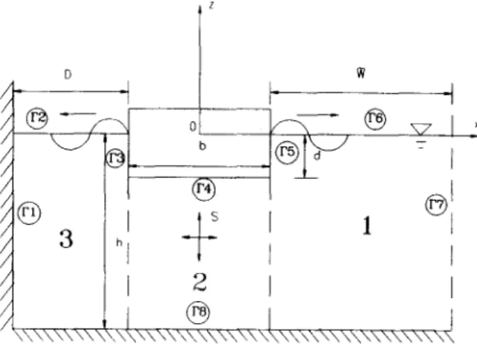
The problem of a rectangular structure oscillating in periodic motion at the water surface, as depicted in Fig. 1, will be studied. The width of the structure is b, and the submergence depth d. The water depth is h. An inertial, Cartesian coordinate system is chosen such that the origin of the x-axis is at the center of symmetry of the structure. The positive x points to the right, and the positive z points upwardly. The sidewall is D distance away

D

z

//

-I

S@

S

:3

h I

/ / \ \ \ \ \ \ \ \ \ \ \ L

1 I

2 I

®

1

, \ X \ \ \ \ \ \ \ \ \ \ \ \ \ \ \ \ \ \ \ \ \ \ \ \ X \ \ \ \

(3)

Hydrodynamic coefficients for an oscillating rectangular structure 179

from the structure. A numerical boundary is located at R H S , distance (V away from the structure, so that the semi-infinite domain becomes confined domain.

By making the usually assumptions of classical hydrodynamics, i.e., the fluid is inviscid and incompressible and the flow is irrotational, the fluid motion can be described by a velocity potential function. The velocity potential • can be expressed as

= R e a l [ ¢b(x,z)e -i~q (1)

i = ~-Z-~, and the velocity potential tb(x,z) must satisfy the Laplace equation

V2~b = 0 (2)

the velocity V can be expressed as

= - w , (3)

where V is the gradient operator. The displacement function of the structure motion can be expressed as

= ise -i'~' (4)

where s is the amplitude, to is the oscillating frequency. The frequency to must satisfy the dispersion relation

to2 = g k t a n h ( k h ) (5)

where g is the gravity acceleration, k is the wave number. The velocity potential must also satisfy the following boundary conditions (Dean and Dalrymple, 1984):

1. The free surface boundary conditions: on F2,/'6

b6

to2

-- = -- dp on z = 0 ( 6 )

0z g

2. The boundary condition at the water bottom: on/'8

O~b = 0 on z = - h (7)

On

i.e., the normal velocity is zero on the solid boundary. Where n is the unit normal vector pointing out of the fluid domain.

3. The boundary conditions on the structure surface: on F4,/-'3 and F5

O~b _ -~,, on So (8)

On

where V. is the velocity vector in normal direction on the structure surface, So is the submerged surface of the oscillating body.

4. The boundary condition at the sidewall: o n / ' l ; which is the same as Equation (7), the normal velocity is zero on the solid boundary

(4)

~n~b O ° n x

(

b

)

= - ~ + D

-

(9)

5. The radiation condition: o n / 7 ; this condition expresses that the behavior of an outgoing wave at ~' distance away from the structure.

The free surface elevation ~ can be calculated by using the linearized Bemoulli's equation:

1

~dp

- i w

- - • ( 1 0 )

g ~t g

The dynamic pressure can be expressed as

P = Pfftt = -io~p~ (11)

The vertical wave force acting on the structure can be calculated by integrating the wave pressure along the submerged surface of structure, and is written as

f

F =

PdA = p

~ - dA = -i~op dPdA = -io~pe -i°~t 4~4

(12)

SO

So so So

where p is the density of fluid. The wave force, F, can be reformulated to obtain the added mass coefficient/~, and the damping coefficient, ~. The solving process for/x and ,~ can be written as follows: (Sarpkaya and Isaacson, 1981)

f

a2~ 0~:

F

= - i t o o e - i ' ' t ~/A = / x ~ + ) t ~ (13) So where

a~

~t

is the velocity of the structure,

a2~

Ot 2

is the acceleration of the structure. Let

qb(x,z) = Re(49) + ilm( qb)

where R e

and I,,,

denote real and imaginary parts respectively. Then

= - - i o ) p e -i,,,' ([Re(~) +

ilm(dp)]dA

F

SO

(14)

(5)

Hydrodynamic coefficients for an oscillating rectangular structure 181 and and f _p = /~.,(6)dA (19) S _J So

Note that in accordance with Equation (18) and Equation (19)/z and A are indeed real. The nondimensional added mass coefficient Ca, and the nondimensional damping coefficient Ca will be defined as

/x 1 (Re(th)dA C a - p V - tosV (20) 2 So

if

c~ - - 1m(4,)d4 (21) p(oV (osV So V = bd

is the submerged volume of the oscillating structure. 3. BEM FORMULATION

The boundary element method (BEM) has been used to solve a variety of problems in theoretical hydrodynamics and elasticity theory (Brebbia and Dominguez, 1989). For a boundary value problem in which the free space Green's function, i.e. fundamental solution, is known, the BEM can be used to perform computations only on the boundary of the domain. The effective dimensionality of the problem is reduced by one. Avoiding detailed computations inside the domain makes the BEM method more efficient than the domain type methods.

To utilize the BEM, we must first convert the boundary value problems into an integral equation representation. Using Green's second identity

fr(6Oq-q~

(22)

From Equation (4) it can be seen that 0~

- - ~ - o ) s e - i t o t ( 1 6 )

Ot

02~

Ot 2 _ ito2se-iO,, (17)

From Equation (13) to Equation (15), the added mass and damping coefficients may be defined explicitly as

of

i x = - - Re(qb)dA (18)

COS

(6)

where q is fundamental solution of the goyerning equation, F is the boundary of the solution domain, fZ is the solution domain, ~b is the velocity potential at a selected point of the boundary.

Because the governing equation of the fluid domain is Laplace equation, the fundamental solution is (Greenberg, 1971)

q = ~-~. In (23)

in which r is the distance from the source point to the field point. From Equation (22) any velocity potential 4~j of the boundary is given by

f

= - - - q - dF (24)

2"n- v ~n bn

in which j is the source point, 13 is the internal angle of the source point j.

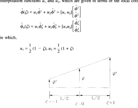
The numerical procedure of the BEM involves dividing the boundary into N segments or elements. To increase the accuracy of the numerical results, the linear element, as shown in Fig. 2, will [ge used to perform computation on the boundary of the domain. Therefore the values of ~b and

3n

at any point on the element can be defined in terms of their nodal values and two linear interpolation functions u~ and u2, which are given in terms of the local coordinates ~, i.e.

+(0

= u , 4 , ' + u 2 6 2 = [u, u21 2 (25) ^

L62j

in which, ul

_{= ~ ( 1 - O, u 2 = ~ ( 1 + 0}

1

1 ... ~?J~ ... " ... J l

7 " . . . . I c y ¢~

(7)

Hydrodynamic coefficients for an oscillating rectangular structure 1 8 3

, ~ varies from - 1 to +1.

For a well-posed boundary value problem, either ~b or tO. or a relation between them is known at all points of the boundaries. Since both th and th. at the radiation boundary are unknowns, the relation between ~b and thn may be built by using the matching conditions of velocity and pressure, at

X--- 4-

, i.e., (Wu, 1987):

c¢

¢h = Ao ig

coshk(h

+ z) ei ~

to cosh(kh)

+ ~ Amcoskm(h + z)e -k.~

m = l

oo

_Aogk

coshk(h

+ z) eik~ _ ~ k,.A,.coskm(h + z)e -k.~

(26) ~b x = ~bn = to cosh(kh)

m = l

the

RHS

is an analytical solution for wave in channel with fiat bottom (Dean and Dalrym- pie, 1984). Since cosh

k(h

+ z) and cos k,. (h + z) (m =1,2 ... ~) are orthogonal functions, one can obtain

0

tocosh(kh)

e_ik~f

v ÷ b f c~ncoShkm(h + z)dz

(27)

Ao -

gkQo

- - h 0 1

- b f

Am

--

kmam e km~w + ~

~bncosk,n(h +

z)dz

(28) - h where 0 Qo = f cosh2k( h +

z)dz

- - h (29) 0 a m =

f

c°s2km(h +

z)dz

--h (30)

in which k., is the wave number of evanescent mode and must satisfy the dispersion relation (Dean and Dalrymple, 1984)

to2 = -gkmtan(kmh)

m = 1,2 ... ~ (31)

in which m is the number of evanescent mode and the calculation requires truncation at some finite value m = M, wherein M is equal to forty in this paper.

Substitution of Equation (27) and Equation (28) into Equation (26), one can establish the relation between t~ and ~bn on the radiation boundary.

(8)

184 Hu-Hsiao Hsu and Yung-Chao Wu 0

icoshk(h + zF) f

~b.coshk(h +

z)dz -

cb(zp) -

kQo

--h 0

f qb~coskm(h + z)dz

h

~ coskm(h + Zp)

m = J

kmQ.,

(32)

Discretizing the above equation by linear element, the equation can be written as

-49i(z,,) + ~ PJckJn = 0 on

F7 (33) J where and )0, fS,

icoshk(h + zp) f~l,

j = 1

kQo

icoshk(h + Zp)_p2 , + icoshk(h + zp)~,

j=/: 1,N

FU =

kQo

icoshk(h + Zp)3~ -~,

j = N

kQo

icoshk(h +

" coskm(h + Zp) •

J~ -

kQo zp) f~ + ~

k,.Q.,

g)ml m = l coskm(h +

icoshk(h + zp)_f~ + ~

Zp)gjm 2

f~; - kOo _{m =} _l kma,o

g~..~ and gJm2 a r e defined by the following two equations ()

J L#~ *~

0

~bncosk,.(h +

z)dz

= - 2 [gJ~l g/m2

- h J

So the boundary value problem can be described completely. Rearranging in such a way that all unknowns are taken to the left hand side and all the knowns are move to the right hand side, then

[A][X] = [B] (34)

where [X] is the vector of unknown ~b and ~bn, [B] is the known vector, [A] is the matrix of coefficients. Equation (34) can be solved by using the Gauss elimination method.

(9)

At comers the flux at both sides may not be unique (so called comer point). To take into account the possibility that the flux at a point before a comer (not necessarily a comer point) may be different from the flux at a point after a comer, two nodes are taken at every comer in the present model. That is replacing the comer node by two different nodes inside each of the two adjacent elements.

4. ANALYTIC SOLUTIONS

4.1. Construction o f the mathematical model

To solve the problem analytically, the problem domain can be divided into three regions as depicted in Fig. 1. (Lee, 1995)

1. Region 1: -___x_< + - h < z < 0 2. Region 2: b [ x l - < ~ , - h - - - z - - < - d 3. Region 3: - + D < - - x < - - 2 ' h < - z < - O

The boundary-value problems describing the three regions can be written as: 1. Region 1 724,~(x,z) = 0

34,1

(DE

b

_ 4,1 o n z = O ; - < - x < - g 2

)

bz 2 - 34,1 34, 2 b 3x - 3x on x =

and radiation condition (4, is outgoing wave). 2. Region 2 V 2 4, 2(x,z) = 0 34, 2 b 3 z - o~s o n z = - d , Ixl --< 34, 2 - 0 o n z = - h 3z (35) (36) (37)

(38)

(39)

(40)

(41)

(10)

186 Hu-Hsiao Hsu and Yung-Chao Wu C#$=+ onx=- ; (42) 4’ = r#$ onx=-- b 2 3. Region 3 v2+3(x,Z) = 0 (43) (44) (45) agJ3 a+2 b ax ax onx=-- 2

ax=0

onx=_

ax

;-_hszsO (47) (48) where +‘, v, C#I’ represent the velocity potential of the three regions.

Note that the velocity and pressure matching boundary conditions for the two neighbor- ing regions has been separated intentionally as shown in Equation (38), Equation (42), Equation (43) and Equation (47). The difficulty of solving the above boundary-value problems is mainly on the region 2 due to the nonhomogeneous boundary conditions (Equation (40) and Equation (43)). Lee’s method (Lee, 1995) will be introduced to solve the nonhomogeneous boundary value problem. The nonhomogeneous boundary-value problem (Equation (39) to Equation (43)), will be separated into two nonhomogeneous problems, one horizontal problem for

and the other vertical problem for 4;

which can be solved analytically.

1. Horizontal homogeneous problem for c#+,*

V2C#&x,z) = 0 _(4% (50)

a44

-=ws onz= -d;

aZ

a+:,

p-0 onz= -h aZ (51) -hszs -d ₍₅₂₎

(11)

Hydrodynamic coefficients for an oscillating rectangular structure 187 b

q b ~ = O o n x = - ~ ; - h <- z <- - d (53)

2. Vertical homogeneous problem for ~bv 2

V2dp~x,z) = 0 (54) bck~' _{az -} 0 on z ₌- d ; _{I x l ~}b ₍₅₅₎ a4,~ - 0 o n z = - h

(56)

bz

b ~b~.=ck 1 o n x = ~ ; - h < - z < - - d (57) b ck 2 = ck 3 on x = - 7 ; - h <- z <- - d (58)

Therefore, the solution to Equation (39) to Equation (43) is equivalent to the sum of the solutions of Equation (49) to Equation (53) and Equation (54) to Equation (58). 4.2. Analytic solutions

By using the method of separation of variables, analytic solutions for the three regions can be obtained.

1. Region 1

b

~1 ~_ Alocosh[k(h + z)]e ik<x- 5 ) + ~] A2.cos[k.(h + z)]e-~.~*-~ )

n = l

(59)

.

where k and k. must satisfy the dispersion relation

co 2 = gktanh( kh ) = - gk.tan( knh ), n = 1,2 ... oo Region 2 4' 2 = 4'~, + 4'~ 4 ~ = ~'..42,sin )t, x - cosh[1,(h + z)] n = l in which and 2cosb[cos(n~r)- 1] nlr /]z. = (A.b)Zsinh[A.(h_d)], h. = ~ - , n = 1,2 ... o¢ b

q~2 = AzoX + B20 + E [A2n ek"~x + b) + B2ne_~.(x_~)]cos[k.( h + Z)]

n = l (60) (61) (62) (63) (64)

(12)

n7T

kn = i-2 n = 1,2,...,z (65)

3. Region 3

4’ =

A,,, cask (2 li + D + x coshk(h + z) + 2 A,,coshk 1 ’ ,,(;+D+x)cosk.(h+z) I, = I

(66)

The unknown coefficients A,,,, A,,, A_<,, and Ban can be determined by using the matching conditions at

(Equation (38), Equation (42)) and at h

x=-~- 2

(Equation (43), Equation (47)), i.e. 1.

a+2 a+!

b

---==

_ax

onx=m~

2

z i

2 &zh,cosh[h,(h + z)] + Am + c k,,(A2,,eknh - B,,2)cos[k,(h + z)]

II = I fl=I x (67) = _{ikA,,cosh[k(h + z)] + z} _{A,,(-k,)cos[k,(h} _{+ z>l} II = I 4J2=#j’ _onx=- ;

$20 + B20 + i (A 2nekrjh + B,,}cos[~,(~ + z>I = A,ocosh[k(h + dl (68)

II = I + 5 A,“COS k,(h + z)l ,I = I 3.

a+2

a+'

b ---==--

_ax

onx= - - 2 5 &&os(h,b)cosh[A,(h + z)] + A,, n=l

(13)

Hydrodynamic coefficients for an oscillating rectangular structure 189 oo

+ ~ k.{A2.-Bz.ek.b}cos[k.(h +

z)] =

A3o(-k)sin[k(D)]

n = l oo cosh[k(h + z)] + ~

A3.(k~)sinh[k~(D)]cos[k.(h +

z)] n = l (69) . b 4, 2 = 4, 3 o n x = - 5

b

~

- ~ Azo + B2o + ~'~ {A~ + B2ne".b}cos[Kn(h +

z)] (70)

n = l

= A3ocos[k(D)]cosh[k(h +

z)] + ~'~

A3.cosh[k~(D)]cos[kn(h +

z)]

n = l

Equation (67) to Equation (70) can now be multiplied by the orthogonal function in their belonging regions, and integrated along the corresponding matching boundary. The algebraic equations thus obtained can be written as

{Mo(1)}A2o + ~2

[A2,.(r,,,e '"b) + B2m(-Km)]{Ml(1,m)}

(71)

m = l

+ a~o(-ik){No(1)}

= - ZA2yAj{N1(1j)}

j = l oo

{Mo(n)}A2o + ~ [Azm(Km eKmb) + Bzm(-Km)]{Ml(n,m)}

(72)

m = l

o~

+ Al(.-,)k,,-llNo(n)} = - ~AzjAjlN,(nj)}

n = 2,3 ...

j = l

A2o (h-d) + B2o(h-d)

+A~o(-1){Mo(1)} + ~

Al(m_tl(-1){Mo(m)} = 0

m = 2

1

oo

+ ~Al~m-l)(-1){Ml(m,n)}

= 0 n = 1,2 ... oo

m = 2

[A2o(- ~) + B2o](h- d) + a3o(-1) { Mo(1) }cos[k(D)]

c~ + Z A3(m - 1)( -- 1 ) { Mo(m) } c o s h [ k m _ 1 (D)] = 0 m = 2 (73) (74)

(75)

(14)

190 Hu-Hsiao Hsu and Yung-Chao Wu

KbF1

]

[A2. +

B2,,e.

] [ ~ ( h - d ) J +

A3o(-1){M,(1,n)}

cos[k(D)] (76)

+ Z A3(m-1)(-

l){Ml(m,n)}cosh[k,,,-l(D)]

= 0 n = 1,2 ...

m = 2

A2o{Mo(1)} + ~ ]

[A2,.Km + Bz.,(-K.,)e""b]{M~(1,m)} + A3o(k)sin[k(D)]

(77)

m = l

-

~ftzjXjcos(Xib){N,(Ij)}

j = l

a2o{Mo(n)} + ~

[a2,.Km + Bz..(-K,.)eKmb]{Ml(n,m)}

m = l

+ a 3 ( . - 1)( - k._ l) {

No(n)

} sinh[k._ ~ (D)] (78)

~e

= - ~AzjA~cos(Ajb){N,(nd)}

n = 2,3 ... oo

j = l

where the symbolic expressions Mo(1), Ml(1, m), No(l), N~ ( 1 , j ) ,

M1 (n, m), No(n), N~(nd)

and Mo(n)

can be written as follows:

d )14o(1) = f cosh[k(h +

z)]dz

(79) --h d

Mo(n ) = f cos[kn_l(h + z)]dz

( n = 2 , 3 . . . 00) ( 8 0 ) - h - d Ml(1,m) =

fcosh[k(h + z)lcostK,.(h +

z)ldz

(81)

--h - d

Ml(n,m) = f

cos[k,_l(h + z)]cos[K.,(h +

z)]dz

(n = 2,3 ... oo) (82)

- h 0

No(I) =

f cosh~[k(h + z)]dz

(83)

h 0

No(n) = f

cos/[kn-t(h

+ z)]dz

(n = 2,3 ... oo) (84)

(15)

Hydrodynamic coefficients for an oscillating rectangular structure 191 - d N~(1 j ) = f cosh[k(h + z)]cosh[Aj(h + z)]dz (85) --h - d _/* Nl(nd) = [ cos[k~_~(h + z)]cosh[Aj(h + z)]dz (n = 2,3 ... ~) (86) - h

Equation (71) to Equation (78) can now be used to solve for the coefficients Al~, A2",

B2~ and A3n; n =0, 1, 2 ... oo. The vertical wave force acting on the structure can be

calculated by th 2 and ~b~, of the region 2, i.e.

t ~ 2 = ¢ ~ 2 e - i ' ~ t = [ t ~ 2 + ~b2le -'°" (87)

3 ~ 2

P = ~ = -itopdpZe -i'°' = - i t o p [ 6 2 + ~b2]e -;°" (88)

F l ~ = ~ = faoPdA = -itope-'~fao[th 2 + th2v]dA = fe - ' ~ (89) where

f = -pro{ ~, ,42~cosh[An(h-d)] c°s[Anb]- 1 _{: 1} _X~ _{( 9 0 )} ekn b - 1

+ B2ob + ~ (a2~ + B2~) ~ c o s [ k ~ ( h - d ) ] ~ n = l

The wave force (F) expression shown in Equation (89) can be reformulated to obtain the nondimensional added mass coefficient Ca, and the nondimensional damping coefficient Ca, R , { f } C a - - - (91) pstobd l m { f } Ca - pstobd (92)

where R, and Im denote real and imaginary parts respectively. 5. NUMERICAL RESULTS AND DISCUSSION

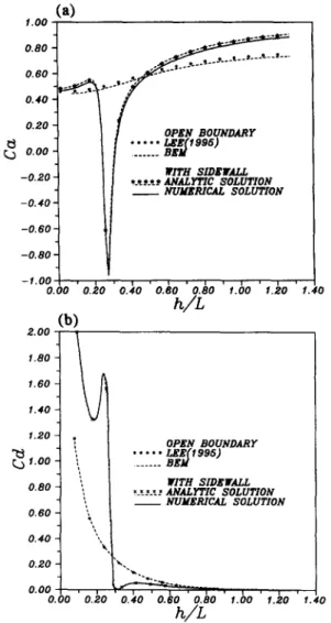
In this paper, we study the heave and the sway problem of a floating rectangular structure in water of finite depth with one side of the boundary is a vertical sidewall and the other boundary is an open boundary. This problem has not been solved by analytical or numerical method and no experimental data in the literature. To prove the accuracy of the present linear element BEM solution and analytical solution, the two side open boundary problem of Lee (1995) has been recomputed and compared to the present results. The geometry parameters of Lee's two examples are (h/b =3.0, d/h =0.4), (blh =0.4, hid =3.0), and the water depth h =1.0 m. The computed dimensionless added mass, Ca, and damping coefficients, Ca, are presented as function of relative water depth h/L, L is the wave length

(16)

192 Hu-Hsiao Hsa and Yung-Chao Wu

of wave generated by oscillating rectangle, and are plotted in Fig. 3 and Fig. 4. The comparisons indicate that the present numerical results of linear BEM agree very well with Lee's analytical solution (Lee, 1995).

The effect of sidewall on Ca and

Cd

will be examined. The problems we consider has the same scale as Lee's (Lee, 1995), but the open LHS boundary is changed to a vertical sidewall, as shown in Fig. 1. Assuming that the clearance between sidewall and rectangle is D =0.2h, numerical results based on linear BEM and analytical method are presented as function of relative water depth and are plotted in Fig. 3 and Fig. 4 again. Both added mass and damping coefficients change rapidly when

h/L

close to 0.25. This is the typical

(a)

0.80 0.60 0 . 4 0 ~ 1 " 0.20 OPEN BOUNDARY ~) . . . I ~ E ( f 995) o.oo ... B E M W I T H SlDEVfALL - 0 . 2 0 *.*..*.*:. ANALYTIC SOLUTION _ _ NUMERICAL SOLUTION - 0 . 4 0 - 0 . 8 0 - 0 . 8 0 o o o o ~o o ~o o ~o o bo I bo 1~o 14o

h/L

(b) 2.00 1.80 1.60 1.40 1.20 '. O P E N BOUNDARY 1.oo ... W I T H SIDEF{ALL 0.80 ,.,. "._".." A N A L P F I C S O L U T I O N _ _ N U M E R I C A L S O L U T I O N o eo ,, O. 40 'k, 0.20

0.00 i ' ~ - ,

. . . . . , 0,00 0 . 2 0 0.40 0.60 0 . 8 0 1.00 1,20 1.40

h/L

Fig. 3. Dimensionless added mass and damping coefficients for a rectangular structure heaving in calm water.

(17)

(a)

t.00 0.80 - 0.60 0 . 4 0 o . e o o~,E~r a o u t c ~ n Y . . . 8t~z~m(1996 ) r,~ 0.00 . . . WITH SIDEFI.I,L - 0 . 2 0 *_*__*.*_.* A N A L Y T I C 3 0 L U T I O N ' NUMffPJCAL SOLLTTIOH -0.40 - -0,60- - 0 . 8 0 ! -1.00

o . o o ' o.~,o ' o.,~o ' o.~o ' o.~o .1.00 1.20 . . .

h/L

(b)

2.00 1 . 8 0 - 1 . 6 0 -. 1.40 - 1 . 2 0 - ,00 : I 0.80 t 0.60 '",,, 0 . 4 0 - 0.20 "~', 0.00 " - - '

o.oo 'o.bo o..~o

h/L

1.40 O P E N B O U N D A R Y WITH SID.ffWAI.,L ~,_,_.,.,--, ANItLPI"IC S O L U T I O N _ _ N U M E R I C A L S O L U T I O N

o . ~ o ' o . ~ o ' 1.bo ' 1.bo ' 1.4o

Fig. 4. Dimensionless added mass and damping coefficients for a rectangular structure heaving in calm water.

(hid =3.0, blh =0.4, DIh =0.2)

resonant behavior. The present results indicate the important effect of sidewall on the hydrodynamic coefficients.

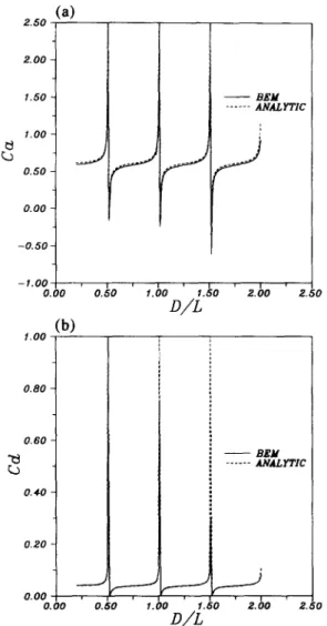
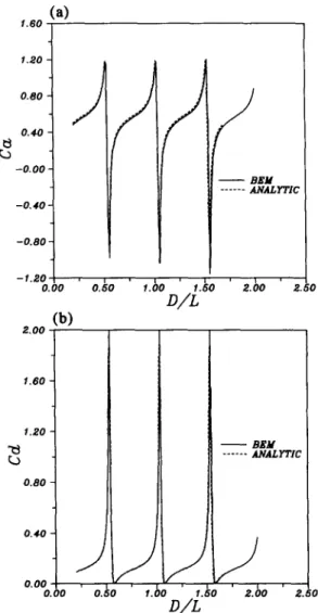
In the following, the important effect of clearance on the hydrodynamic coefficients will be examined in detail. Define the relative clearance as DIL. Numerical results of linear

BEM and analytical method are plotted in Fig. 5a and b for Ca and Ca respectively. In

Fig. 5 the added mass and damping coefficients are shown as function of relative clearance,

D/L, for h/L ---0.5. We fined that both Ca and Ca values have great change when DIL is

equal to 0.5, 1.0 and 1.5. This phenomenon is called resonance, the same as harbor seich- ing. Due to the reflection of vertical sidewall, wave energy is accumulated in the region

(18)

194 Hu-Hsiao Hsu and Yung-Chao Wu (a) 2.50 2.00 1.50 1.00 0.50 0.00 - 0 . 5 0 - 1 . 0 0 0.00 (b) 1 . 0 0 - - B E M . . . ANALYTIC

J

o./so ,.bo ,.~o a.bo s.5o

D/L

0.80 0.60 0.40 - - B E M . . . A N A L Y T I C 0.20 0.00 , , , 0.00 0.50 1.00 1.50 2.00

D/L

2 . 5 0

Fig. 5. Dimensionless added mass and damping coefficients for a rectangular structure heaving in calm water.

(h/d =3.0, b/h =0.4, h/L =0.5)

between sidewall and structure. T o further prove this resonant behavior, the dimensionless

added mass and damping coefficients have been computed and plotted in Fig. 6a and b

for tdL =0.3. The resonance phenomena appear at the same relative clearance as before,

i.e., D/L =0.5, 1.0 and 1.5. We conclude that if the clearance D is integral timms o f half

wave length, L/2, the resonant behavior will appear, and the hydrodynamic coefficients will change rapidly.

In addition to the heave motion, w e also examine the added mass and damping coef- ficients for a rectangular structure oscillating in a s w a y motion in calm water with finite depth. At first, the numerical results o f Ca and Ca are presented as function o f relative

(19)

(a)

t . 6 0 1.20 0 . 8 0 0.40 e~ - 0 . 0 0 - - 0 , 4 0 " - 0 . 8 0 - 1 . 2 0 0.00

(b)

2. OO

)/

_/

/

- - B E M . . . A N A L Y T I C

o.ko 1.bo 1.6o 2,bo z.5o

D / L 1.60 1.20 0.80 - - B E M . . . IdCI.tI,]'TIC

o.,o ) y , / )

0.00 , , 0.00 0.50 1.00 1.50 2.00 2.50

D/L

Fig. 6. Dimensionless added mass and damping coefficients for a rectangular structure heaving in calm water. (h/d =3.0, b/h =0.4, h/L =0.3)

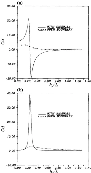
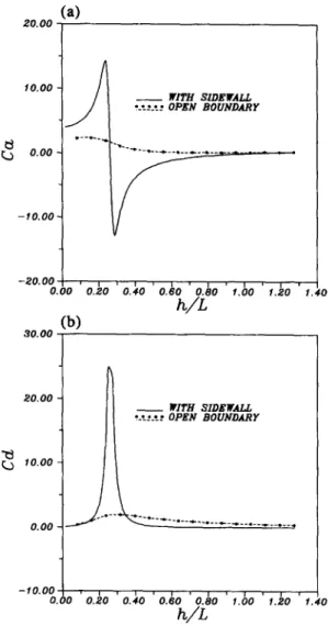
depth h/L and are plotted in Fig. 7 and Fig. 8. Both Ca and Ca change rapidly when h/L

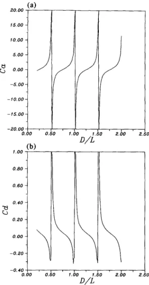
close to 0.25. These results indicate the important effect of sidewall. The important effects of clearance on C= and Ca are shown in Fig. 9 and Fig. 10 for h/L =0.5 and h/L =0.3

respectively. Again the resonance phenomena appear as the clearance is integral times of half wave length, and the hydrodynamic eoefticients change rapidly.

6. CONCLUSIONS

The BEM with linear element has been established to study the hydrodynamic properties of rectangular structure oscillating on water of finite depth. The accuracy of the BEM is

(20)

196

30. O0

Hu-Hsiao Hsu and Yung-Chao Wu

(a)

20.00- 10.00. 0.00 - -10.00- _ _ ~[ITH S I D E W A L L • .'..'_'_." O P E N B O U N D A R Y -20.00 . . . . .

o.oo o.;zo o.~o 'o.~o o.~o ,.bo 1.~o 1 4 o

h/L

(b)

40.00 t 30.00 1 20. O 0 10.00 0.00 _ _ W I T H S I D E W A L L ,_.__._.__. O P E N B O U N D A R Y -I0.00 . . . . . . .

o.oo o.~o o~o o.~o o.~o ,.bo I~O ,.4o

h/L

Fig. 7. Dimensionless added mass and damping coefficients for a rectangular structure swaying in calm water.

( h l b =3.0, d l h ---0.4, D I h ----0.2)

proved by comparing numerical results of BEM and analytical method. Negative added mass and sharp peaks in the added mass and damping coefficients have been found when one side of the open boundary is replaced by sidewall. Resonant behavior will appear when the clearance between sidewall and structure is integral times of half wave length of wave generated by oscillating structure. The hydrodynamic coefficients of any shape structure oscillating on water can be examined by using the present numerical technique. This work is supported by the National Science Council, Republic of China, under grant No. NSC-84-2611-E-009-002.

(21)

Hydrodynamic coefficients for an oscillating rectangular structure

(a)

20. O 0 197 1 0 . 0 0 Y 0 . 0 0 * - - " ' ~ ""'~'-°--~--, ... ~ . . . = - 1 0 . 0 0 - 2 0 . 0 0

o.oo ' o.~o ' o . ; o ' o.~o ' o.~o ' ,.oo' ' , . ~ o ' 1.,~o

h/L

(b)

30. O0 E,~ I0.00 20. O 0 _ _ W I T H S I D E W A L L ~.~._*.*_.* O P E N B O U N D A R Y I

/ _ _

o o o ... -10.00

o.oo 'o.~o ' o.~o ' o.~o 'o.~o ' 1.bo ' 1.~o ' ,.40

h/L

Fig. 8. Dimensionless added mass and damping coefficients for a rectangular structure swaying in calm water.

(hid =3.0, blh =0.4, DIh =0.2)

R E F E R E N C E S

Bai, K. J. and Yeung, R. W. 1974. Numerical solutions to free-surface flow problems. Tenth Symposium on Naval Hydrodynamics, Cambridge, Mass., pp. 609--633.

Brebbia, C.A. and Dominguez, J. 1989. Boundary Elements: An Introductory Course. McGraw-Hill.

Black, J.L., Mei, C.C. and Bray, M.C.G. 1971. Radiation and scattering of water waves by rigid bodies. J. Fluid

Mech, 46, 151-164.

Dean, R.G. and Dalrymple, R.A. 1984. Water Wave Mechanics for Engineers and Scientists. Greenberg, M.D. 1971. Application of Green's Function in Science and Engineering. Prentice-Hall.

Havelock, T. H. 1955. Waves due to floating sphere making periodic heaving oscillations. Proc. Royal Soc. Lond. A231, pp. 1-7.

Hulme, A. 1982. The wave forces on a floating hemisphere undergoing forced periodic oscillations. J. Fluid

(22)

198 Hu-Hsiao Hsu and Yung-Chao Wu "0 rO 1.00 0,80

(a)

2 0 . O 0 15.00 - 10.00 / 5.00

/

o . o o - f - 5 . 0 0 - - I 0 , 0 0 - - 1 5 . 0 0 - -20.00 0.00 0.50

(b)

0 . 6 0 0.40 0.,80 0.00 -0.20 -0.40 0.00 rO 1.00 1.5d 2,00

z /L

,?,.50

o.ho l.bo ,.ho e.bo e so

D J L

Fig. 9. Dimensionless added mass and damping coefficients for a rectangular structure swaying in calm water. (h/d =3.0, blh --0.4, tdL ---0.5)

Kim, W.D. 1965. On the harmonic oscillations of a rigid body on a free surface. J. Fluid Mech. 21, 427-451. Lebreton et al., 1966: Author: please supply full ref. or delete in text.

Lee, J.F. 1995. On the heave radiation of a rectangular structure. Ocean Engng. 22, 19-34.

Nestegard, N. and Sclavounos, P.D. 1984. A numerical solution of two-dimensional deep water wave-body problems. J. Ship Res. 28, 48-54.

Sarpkaya, T. and Isaaeson, M. 1981. Mechanics of Wave Forces on Offshore Structures. Van Nostrand-Reinhold, New York.

(23)

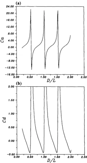
199 1.50

(a)

24. O0 20.00 16.00 12.00 8.00 ¢) 4.00 o . o o - - 4 . O0 - - 8 . 0 0 - - 1 2 . 0 0 - - 1 6 . 0 0 0.00

(b)

2.00

/

1.00 0 . 5 0 0.00 - 0 . 5 0 0.00

/

Hydrodynamic coefficients for an oscillating rectangular structure

,.bo ~.~0 2.bo 2.50

i 0 . 5 0

D/z,

o.~o l.bo 1.5o 2.00 2.50

D/Z`

Fig. 10. Dimensionless added mass and damping coefficients for a rectangular structure swaying in calm water. (h/d =3.0, b/h =0.4, hlL =0.3)

Vantorre, M. 1986, Third-order theory for determing the hydrodynamic forces on axisymmetric floating or submerged bodies in oscillatory heaving motion. Ocean Engineer/rig 13, 339-371.

Wu, Y.C. 1987. Constant Wave Form Generated by A Hinged Wavemaker of Finite Draft in Water of Constant Depth. Proc. of 9th Conf. on Coastal Engineering, Taiwan, R.O.C., pp. 552-569.

Yeung, R.W. 1975. A Hybrid Intesral-Equation Method for Time Harmonic Free-Surface Flows, 1st International Conference on the Ship Hy&odyrmmics, Gaithevsburg, Md., pp. 581-607.