Estimation of the Moments of the Residence Time and First Passage Time from Experimentally Measurable Permeation Parameters via a New Formulation of the Transmission Matrix

Estimation of the Moments of the Residence Time and First Passage Time from

Experimentally Measurable Permeation Parameters via a New Formulation of the

Transmission Matrix

Jenn-Shing Chen,

a,

* Kwei-Tin Yeh,

a

Wen-Yih Chang

a

and James K. Baird

b a

Department of Applied Chemistry, National Chiao-Tung University, Hsin-Chu 30010, Taiwan

b

Department of Chemistry, University in Huntsville, Huntsville, Alabama, AL 35899, USA (Received: Sept. 28, 2013; Accepted: Dec. 23, 2013; Published Online: Apr. 14, 2014; DOI: 10.1002/jccs.201300491)

Siegel’s analysis on membrane transport in the Laplace domain [J. Phys. Chem. 95 (1991) 2556] in terms of transmission matrix, T(s), has been extended to a more useful formulation. This is achieved by combin-ing uses of the matrix transport equations appropriate for void initial condition, or for saturated equilib-rium, or of Dirac delta functional type and the theorem det[T(s)] = 1. This formulation enables us to ex-pand T(s) in power series of the Laplace variable, s, with the expansion coefficients as the algebraic func-tions of the experimentally measurable transport parameters. Utility of the formulation is illustrated in the estimation of the experimentally inaccessible time moments for the first passage or residence times. It was also applied to the percutaneous drug delivery to obtain from the experimental data. The higher moments of the time lag or time lead using a graphic method.

Keywords: Transmission matrix; Membrane transport; Percutaneous drug delivery. INTRODUCTION

Permeation transport across membranes is of great importance in science and technology, and has played a crucial role in such diverse fields as chemical sensors,1,2 controlled release,3,4 separation processes,5 protection against pollution,6electrodialysis,7to name just a few. In practical applications, three modes of membrane transport are employed:8(a) absorptive permeation, where the initial activity within the membrane is zero and the activities at the upstream and downstream faces are at a constant level

a0and zero, respectively; (b) desorptive permeation, where the initial condition is of saturated equilibrium with activ-ity a0throughout the whole membrane. If the activity is a0 at the upstream face, zero at the downstream face, then we have forward desorptive permeation; and if, on the other hand, the boundary conditions at two faces are exchanged, then we have backward desorptive permeation; (c) desorp-tion, where the initial activity a0prevails throughout the whole membrane and the boundary conditions at both faces are kept at zero activity. For heterogeneous membranes, where the diffusivity D(x) and partition coefficient K(x) depending on position, the permeation can be mathemati-cally described by the Smoluchowski equation,9-11 ¶

¶tr( , )x t = ¶ ¶xD x( )K x( ) ¶ ¶x r( , ) ( ) x t

K x . The complete knowledge about

the membrane permeation entails the full time-dependent solution to the diffusion equation subject to appropriate boundary and initial conditions. Unfortunately full, analyt-ical solution is seldom obtained except for some simple, trivial cases. Thus one is usually satisfied with obtaining a few diffusion parameters characteristic of the permeation such as permeation (P), time lag (tL) for absorptive and

time lead (t₊) for desorptive permeation and their higher moments.12,13All these permeation parameters can be ob-tained directly from the suitably designed experiments. For details, see section 4 below. Theoretically, they can also be formulated via the Taylor expansion of the transmission matrix, T(s), in power series of s with the expansion coeffi-cients expressed in terms of the repeated integrals of [K(x)D(x)]-1and K(x)14or by the method of repeated inte-gration of the diffusion equation.9,15However, these formu-lations are useful only in the cases where the functions K(x) and D(x) are known beforehand.

Another concern about diffusion transport is the mo-ments of the first passage time10,11,16and residence time.17,18 As a rule, neither is obtainable directly from the experi-ments. Mathematically the former can be obtained by solv-ing the adjoint (or backward) diffusion equation10,11and the latter by the Green’s function of the diffusion equation.17,18 Again these tasks are feasible only when K(x) and D(x) are known ahead of time.

In this communication we will contrive a device which makes it possible to estimate the moments of the res-idence time and first passage time from permeation param-eters obtained directly from suitably designed permeation experiments. Using the measurable permeation parameters of component laminae, it is also useful for the estimation of various time moments of a composite laminate. This device is the Taylor expansion of the transmission matrix, T(s), in power series of s with the expansion coefficients expressed in terms of the measurable parameters: permeability, time lag and time lead and their higher moments. With this de-vice, evaluation of most of the diffusion time moment amounts merely to a task of algebraic manipulation. The rest of this article will be organized as follows: Section 2 presents the matrix transport equations for void and satu-rated equilibrium initial conditions. In conjunction with the theorem det[T(s)] = 1, we are able to correlate the fluxes of various modes with the matrix elements to express the ex-pansion coefficients of T(s) in terms of various permeation time moments. Section 3 illustrates the application of this device to the time moments of the first passage time, resi-dence time, and percutaneous drug delivery. Section 4 sug-gests a graphical method for the treatment of the experi-mental data to obtain the time moments for absorptive and desorptive permeation and finally the last section gives a concluding remark.

TAYLOR EXPANSION OF T(s) IN TERMS OF PERMEATION PARAMETERS

We start with the matrix transport equation for void initial concentration within the whole membrane14,19-21

(1)

This equation relates the pair (activity, a$ ( )u s, and flux,

$ ( )

Ju s) in the Laplace domain at the upstream face to the

counterpart,a$ ( )d s and $ ( )Jd s, at the downstream face. For

membrane absorptive permeation,a$ ( )u s = a

s

0

anda$ ( )d s = 0

are the boundary conditions. The permeation flux at the downstream face is calculated to be

(2)

where the superscript (a) is indicative of “absorptive”. In terms of $Jd( )

a

( )s , the diffusion parameters steady-state

per-meability (P), time lag (tL) and its second and third

mo-ments (tL

( )2 , tL

( )3

) for absorptive permeation can be defined as shown in Eqs. (3)-(6). A subsequent use of Eq. (2) leads to (3) (4) (5) (6) where Jd ss a , ( )

is the steady-state flux for absorptive perme-ation. Equations (4)-(6) are equivalent to the statement that

tL, tL

( )2 and tL

( )3

are the first, second and third time moments based on the distribution (d

dtJd a ( ) ( )t )/Jd ss a , ( ) , respectively. On rearranging Eqs. (3)-(6), the Taylor expansion ofT s₁₂( )can be represented in terms of the diffusion parameters of the absorptive permeation by

(7)

where the definition ofbi (i = 0, 1, 2, 3) is self-explanatory

in Eq. (7).

To find a similar series for T22( ) the forward desorp-s

ú û ù ê ë é ú û ù ê ë é = ú û ù ê ë é = ú û ù ê ë é ) ( ˆ ) ( ˆ ) ( ) ( ) ( ) ( ) ( ˆ ) ( ˆ ) ( ) ( ˆ ) ( ˆ 22 21 12 11 s J s a s T s T s T s T s J s a s T s J s a u u u u d d s a s T s J_da 0 12 ) ( ) ( 1 ) ( ˆ ₌ -) ( 1 0 lim ) ( ˆ 0 lim 12 0 ) ( 0 ) ( , s T s a s J s s a J P a d a ss d ® -= ® = º ) ( ) ( 0 lim ) ( ˆ 0 lim 12 12 ) ( , ) ( s T s T ds d s J s J s ds d s t _a ss d a d L = _® -® º ï ï þ ïï ý ü ï ï î ïï í ì -÷÷ ÷ ÷ ø ö çç ç ç è æ ® = ® º ) ( ) ( ) ( ) ( 2 0 lim ) ( ˆ 0 lim 12 12 2 2 2 12 12 ) ( , ) ( 2 2 ) 2 ( s T s T ds d s T s T ds d s J s J s ds d s t a ss d a d L ) ( ) ( 0 lim 2 12 12 2 2 2 s T s T ds d s t_L ® -= ) ( , ) ( 3 3 ) 3 ( ) ( ˆ 0 lim a ss d a d L J s J s ds d s t -® º ï ï þ ïï ý ü ï ï î ïï í ì -+ ÷÷ ÷ ÷ ø ö çç ç ç è æ ® = ) ( ) ( ) ( ) ( 6 ) ( ) ( ) ( ) ( 6 0 lim 12 12 12 12 2 2 12 12 3 3 3 12 12 s T s T ds d s T s T ds d s T s T ds d s T s T ds d s ) ( ) ( 0 lim 6 6 12 12 3 3 3 ) 2 ( s T s T ds d s t t t_{L L L} ® + -= L -+ -= 3 ) 3 ( ) 2 ( 3 2 ) 2 ( 2 12 6 6 6 2 2 1 ) ( s P t t t t s P t t s P t P s T L L L L L L L L -= 3 3 2 2 1 0 b s b s b s b

tive permeation mode is employed, which in turn requires the transport equation for initial saturated equilibrium14,21

(8)

witha$ ( )d s = 0,a$ ( )u s = a

s

0

, appropriate for this mode of per-meation, the permeation flux at downstream face is given by

(9)

where the superscript (d) is indicative of “desorptive”. Again we can define the forward time lead t₊, and its higher moments in terms of $Jd( )

d

(s) and use Eq. (9) to obtain

(10)

(11)

(12)

The subscript, +, in t₊, t₊( )2 and t₊( )3 is used to specify the permeation in the forward direction. With the fact that steady-state permeabilities for absorptive and desorptive permeation are identical, and after inserting Eq. (9) into Eqs. (10)-(12), the Taylor expansion ofT s22( )can be

repre-sented after rearrangement by

(13) where t₊= tL - t+, t+ ( )2 = tL ( )2 _{- t} + ( )2 and t₊( )3 = tL ( )3 _{- t} + ( )3 , and the definition ofdi for i = 0, 1, 2, 3 is self-explanatory.

To find the Taylor expansion of T₁₁( ) , we use thes

backward desorptive permeation flux, $ ( )Ju s d

, which is cal-culated using Eq. (8) witha$ ( )d s =

a s

0

anda$ ( )u s = 0 to obtain

(14)

In a fashion similar to that used to obtain T22( ) in Eq. (13),s

we find (15) where t_-= t_L- t_-, t_-( )2 = t_L( )2 _{- t} -( )2 and t-( )3= tL ( )3 _{- t} -( )3, with

t_-being the time lead for backward desorptive permeation and t_-( )2

and t_-( )3

its second and third moments, respectively. For n = 0, 1, 2, 3 theaiare defined in Eq. (15).

A further application of the theorem21

(16)

allows us to obtain for T21( ) the Taylor series expansions

(17) Again, the definition ofg_i(i = 1, 2, 3) is self-explanatory.

Results collected from Eqs. (7), (13), (15) and (17) represent the Taylor expansion of T(s) in power series of s with the coefficients expressed in terms of permeation time moments which are measurable from the experiments. They can be looked upon as a supplement to the Taylor ex-pansion of T sij( ) in power series of s with coefficients

ex-pressed in terms of repeated integrals of K(x) and [k(x)D(x)]-1as revealed in reference.14These representa-ú ú û ù ê ê ë é -ú û ù ê ë é = ú ú û ù ê ê ë é -) ( ˆ ) ( ˆ ) ( ) ( ) ( ) ( ) ( ˆ ) ( ˆ 0 22 21 12 11 0 s J s a s a s T s T s T s T s J s a s a u u d d s a s T s T s J_dd 0 12 22 ) ( ) ( ) ( ) ( ˆ ₌ -÷÷ ÷ ÷ ø ö çç ç ç è æ -® = -® = + _{( )} ) ( ) ( ) ( 0 lim ) ( ˆ 0 lim 22 22 12 12 ) ( , ) ( s T s T ds d s T s T ds d s J s J s ds d s t _d ss d d d ) ( , ) ( 2 2 ) 2 ( ) ( ˆ 0 lim d ss d d d J s J s ds d s t ® = + ï ï þ ïï ý ü ï ï î ïï í ì ÷÷ ÷ ÷ ø ö çç ç ç è æ + -® = 2 12 12 22 22 12 12 12 12 2 2 22 22 2 2 ) ( ) ( 2 ) ( ) ( ) ( ) ( 2 ) ( ) ( ) ( ) ( 0 lim s T s T ds d s T s T ds d s T s T ds d s T s T ds d s T s T ds d s ) ( , ) ( 3 3 ) 3 ( ) ( ˆ 0 lim d ss d d d J s J s ds d s t -® = + ï ï î ïï í ì ÷÷ ÷ ÷ ø ö çç ç ç è æ -® = 2 12 12 22 22 12 12 2 2 12 12 22 22 2 2 12 12 ) ( ) ( ) ( ) ( 6 ) ( ) ( ) ( ) ( 6 ) ( ) ( ) ( ) ( 3 0 lim s T s T ds d s T s T ds d s T s T ds d s T s T ds d s T s T ds d s T s T ds d s 3 12 12 12 12 3 3 22 22 3 3 12 12 2 2 22 22 ) ( ) ( 6 ) ( ) ( ) ( ) ( ) ( ) ( ) ( ) ( 3 ÷ ÷ ÷ ÷ ø ö ç ç ç ç è æ + + -+ s T s T ds d s T s T ds d s T s T ds d s T s T ds d s T s T ds d L + -+ + -+ + = + + + + + + + 3 ) 2 ( ) 2 ( 2 ) 3 ( 2 ) 2 ( 22 6 3 3 6 2 2 1 ) (s t s t t t s t t t t t t t s T L L L L L + + + + = 3 3 2 2 1 0 d s d s d s d s a s T s T s J_ud 0 12 11 ) ( ) ( ) ( ) ( ˆ ₌ L + -+ + -+ + = - - - -- 3 ) 2 ( ) 2 ( 2 ) 3 ( 2 ) 2 ( 11 6 3 3 6 2 2 1 ) (s t s t t t s t t t t t t t s T L L L L L + + + + = 3 3 2 2 1 0 a s a s a s a 1 ) ( ) ( ) ( ) ( )] ( det[T s =T₁₁ sT₂₂ s -T₁₂ sT₂₁ s = 2 ) 2 ( ) 2 ( 21 [2 ] 2 ] [ ) (s P t t s P t t t t s T =- ₊+ _- - _{+ -}- ₊ - -L + + -+ -P₆[t+(3) t-(3) 3t+(2)t- 3t+t-(2) 6tLt+t-]s3 L + + + = 3 3 2 2 1s g s g s g

tions are the central result of the article and will be applied to the estimation of the time moments of the following problems.

APPLICATIONS

As the first example, we consider the first passage time for a particle initially located at x0 between a reflect-ing face xu and an absorbing face xd, xu < x0< xd.

11,16 Solv-ing this problem requires the matrix transport equation for an initial condition ofd-function type14,19

(18)

where T*( ) is the transmission matrix for the subdomains

from x0to xd. After substitution of $ ( )Ju s = 0 anda$ ( )d s = 0

into Eq. (18), the flux escaping from the face x_d is calcu-lated to be

(19)

The mean first passage time can be represented by

(20)

where the denominator represents the initial total amount which is equal to unity. Putting Eq. (19) into Eq. (20) fol-lowed by expanding the transition matrix elements in terms of Eqs. (7), (13), (15) and (17), we obtain

(21)

Here the quantity associated with the superscript * denotes the fact that this quantity is to be specified to the sub-do-main, x0< x < xd. The second moment of first passage time

is also easily calculated by

(22) where t₊* = tL * _{- t} + * and t₊( )*2 = tL ( )*2 _{- t}

+( )*2 . Thus with each quantity on the right-hand sides of Eqs. (21) and (22) being experimentally accessible,m1andm2can be estimated.

The second example goes to the estimation of the mo-ments of the residence time for the first example.17,18These residence time moments are not measurable directly from experiments. The residence time is related to the Green’s function $ ( , |G x s x₀)associated with the diffusion equa-tion.14,18Such a Green’s function can be constructed by the following strategy. The diffusion domain is partitioned into three sub-domains labeled by A, B, C. A is from xu to x, B

from x to x0and C from x0to xd. The matrix transport

equa-tion between the xu and xd, where the initial location x0 is confined, reads19

(23)

The transport equation for the sub-domain between xu and

x, where the particle is not initially located, reads

(24)

The superscript capitals A, B, C signify the regions with which the transmission matrices associate and the subscript x denotes “at the interface x”. Substituting the boundary conditionsa$ ( )_d s = 0 and $ ( )J_u s = 0,a s$ ( )_x is found from Eqs. (23) and (24) to be

(25)

Upon using Eqs. (7) and (15), we obtain

(26)

But it should be noted that it is the concentration Green’s function which gives residence time not the activity. With the relation14,19,20a x s =$( , ) $( , )

( ) r x s

K x we find the mean

resi-dence time at x for infinitely long observation time to be

(27)

and its second moment to be ú û ù ê ë é + ú û ù ê ë é = ú û ù ê ë é 1 0 ) ( ) ( ˆ ) ( ˆ ) ( ) ( ˆ ) ( ˆ _* s T s J s a s T s J s a u u d d ) ( ) ( ) ( ) ( ) ( ) ( ˆ 11 * 12 21 * 22 11 s T s T s T s T s T s J_d = -) ( ˆ 0 lim ) ( ) ( 0 0 1 J s ds d s dt t J dt t J t d d d ® -= =

ò

ò

¥ ¥ m * * 1=[++ -] -t+ P P t t m ) ( ˆ 0 lim ) ( ) ( 2 2 0 0 2 2 J s ds d s dt t J dt t J t d d d ® = =

ò

ò

¥ ¥ m )] ( 2 2 [ * t 2 _L* ₊*- ₊(2)*+ ₊(2)+ _-(2)+ _-2- * ₊+ -= t t t t t t P P t t _L ú û ù ê ë é + ú û ù ê ë é = ú û ù ê ë é 1 0 ) ( ) ( ˆ ) ( ˆ ) ( ) ( ˆ ) ( ˆ _{( ) ( )} s T s J s a s T s J s a _C u u ABC d d ú û ù ê ë é = ú û ù ê ë é ) ( ˆ ) ( ˆ ) ( ) ( ˆ ) ( ˆ _{( )} s J s a s T s J s a u u A x x ) ( ) ( ) ( ) , ( ˆ ) ( ˆ ) ( 11 ) ( 11 ) ( 12 s T s T s T s x a s a ABC A C x = =

-{

( ) 1 ) , ( ˆ ) ( ˆ ( ) 1 ) ( 1 ) ( 1 ) ( 0 ) ( 2 ) ( ) ( ) ( ) ( ) ( A ABC ABC C C C ABC A C L C x s P t t t P s x a s a = = + +- -- + b +b a a -a

}

+L -- ( ) 2 1 ) ( 1 ) ( 1 ) ( 2 ) ( 2 ) ( 0 ( ) ( ) s A ABC C A ABC C _{a a b a a} b ) ( ) ( ) ( ) ( ) ( ) ( _C A C L ABC P t t t x K x = - - - -t

(28)

The value of K(x) may be obtained from the experimentally measurable permeabilityD x K x

x

( ) ( )

D and time lag ( ) ( ) Dx D x 2 6 for

a slice of material between x and x+ D , with Dx thin enoughx

to be considered homogeneous. In the case of x>x0, a simi-lar calculation yields

(29)

(30)

where the sub-domain A¢ is from xuto x0, B¢ from x0to x, C¢ from x to xd. Thus we have demonstrated that

experimen-tally inaccessible residence time moments can be estimated from the experimentally measurable quantities.

As a third example, consider a membrane initially in a state of saturated equilibrium at a constant activity, a₀, that undergoes desorption leakage from either ends. The tradi-tional desorption experiment measures the total release from both sides, hence, is unable to give the release time moments for a particular side. This difficulty, however, can be overcome by our method. The Laplace transform of the escaping flux at the downstream face is found to be

(31)

by substitutinga$ ( )u s =a$ ( )d s = 0 into Eq. (8) as required for

desorption experiment. If Eqs. (7) and (13) are used, $ ( )Jd s

can be expanded as a power series in s to be

(32)

It immediately follows upon using Eqs. (7) and (17) that the first time moment, td, for release from the downstream face

is

(33)

upon using Eqs. (7) and (17). The second moment td

( )2 for release from the downstream face is found to be

(34)

Similar calculation on the first (tu) and second (tu

( )2 ) mo-ments of the release time from the upstream face gives

(35)

(36)

Again, the time moments for escaping from a particular boundary, which is experimentally inaccessible, can be es-timated from the experimentally accessible permeation pa-rameters.

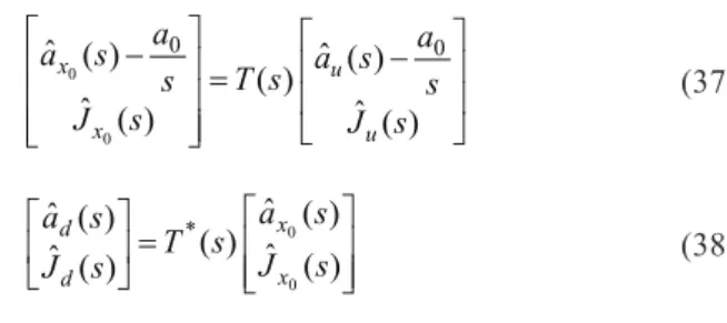
As the last example, we consider a percutaneous drug delivery from a patch matrix attached to the skin. The ma-trix is homogeneously saturated with the drug. During ad-ministration, the drug molecules diffuse through the matrix and skin (specifically, stratum cornea) into the tissue. The configuration of the permeation system is sketched in Fig. 1, indicating that the upstream face is reflecting, i.e., imper-meable, and the downstream face is absorbing. The matrix transport equations for this drug delivery system are as adapted from Eqs. (1) and (8).

(37)

(38)

The quantity with the subscript u (0, d) is that at the face xu

= ) ( ) 2 ( _x t )] ( ) ( ) ( [ ) ( 2 1( ) ) ( 1 ) ( 1 ) ( 2 ) ( 2 ) ( 0 ) ( 1 ) ( 1 ) ( 1 ) ( 0 ) ( 2 A ABC C A ABC C A ABC ABC C C x K b +b a a -a -b a -a -b a -a ïþ ï ý ü ïî ï í ì + -= - -) ' ( ) ' ( ) ' ' ( ) ' ' ( ) ' ' ( ) ' ' ' ( ) ( ) ( B B L C B B A C B L C B A P t P t t t x K x t ] ( [ ) ( 2 ) ( ₂( ' ') ₂( ') ₀( ' ') ₁( ' ' ') ₁( ' ' ') ₁( ' ') ) 2 ( BC B BC ABC ABC AB x K x b b b a a a t = - + -] ( ) ( [ ) ( 2K x b₀(B'C')a₂(A'B'C')-a(₂A'B') +b₁(B'C')a₁(A'B'C')-a₁(A'B') -s a s T s T s J_d 0 12 22 ) ( ) ( 1 ) ( ˆ ₌ -0 2 3 0 1 2 1 2 1 0 1 2 0 3 2 0 2 0 1 1 2 0 0 1 _] [ ) ( ˆ _{s s s a} Jd = + - + - - + +L b d b d b b d b b d b b d b d b b d + + = -= -® = t 2 ) ( ˆ ) ( ˆ 0 lim (2) 1 2 0 1 t s J s J ds d s t d d d _d d b b + + = + -= ® = t 3 ] [ 2 ) ( ˆ ) ( ˆ 0 lim (3) 2 0 2 1 0 1 1 2 0 2 1 3 2 2 ) 2 ( t s J s J ds d s t d d d b b b b d d b b d d -= t 2 ) 2 ( t t_u -= t 3 ) 3 ( ) 2 ( t t_u

Fig. 1. Lay out of the percutaneous drug delivery, x_u, is

an impermeable boundary, x₀is the interface

between the matrix and stratum cornea, x_dis the interface between stratum cornea and tissue, and is assumed to be absorbing.

ú ú û ù ê ê ë é -= ú ú ú û ù ê ê ê ë é -) ( ˆ ) ( ˆ ) ( ) ( ˆ ) ( ˆ 0 0 0 0 s J s a s a s T s J s a s a u u x x ú ú û ù ê ê ë é = ú û ù ê ë é ) ( ˆ ) ( ˆ ) ( ) ( ˆ ) ( ˆ 0 0 * s J s a s T s J s a x x d d

(x₀, xd). The superscript * is used to specify the quantity in

the stratum cornea. The quantity without * as its superscript is the one which be specified in the patch matrix. Solve

$ ( )

J_d s from Eqs. (37) and (38) after substitutinga$ ( )_d s = 0, $ ( )

Ju s, results in

(39)

The Taylor expansion of $ ( )J_d s in power series of s can be obtained upon using Eqs. (7), (13), (15) and (21) and is found to be (40) with P= g1 (41) (42) (43)

The first moment for the drug delivery is then

(44)

and the second moment is

(45)

where the Greek letters can be found specified in Eqs. (7), (13), (15) and (17).

DATA TREATMENT

The feasibility of this new methodology gears to the permeation parameters: permeability, time lag for absorp-tive permeation and time leads for forward and backward

desorptive permeations and their higher moments. The per-meability, time lag and time lead are usually obtained from the slope and the intercept with the time axis of the linear asymptote for a plot of total release, Q t( ) = J d

t

( )t t 0

ò

,

against time, t (see Fig. 2).22This graphic method can be also extended to the determination of higher moments. From the definition of the n-th moment of the time lag in the Laplace domain, Eqs (4)-(6), which can be transformed into the time domain. After integration by parts, we have

(46)

After arrangement, Eq. (46) becomes

(47) Thus a plot of y= tn d t t t J d

-ò

1 0

( ) against x= will exhibit atn

linear asymptote with a slope J

n d ss,

and an intercept (with

s a s T s T s T s T s T s J_{d *} 0 11 11 * 12 21 12 ) ( ) ( ) ( ) ( ) ( ) ( ˆ + -= 0 2 ) s R s ( ) ( ˆ _{s P Q a} J_d = + + +L ) ( 1 1* 0* 1 1 2 g a a b g g - + + = Q ) ( _{2 1 1}* ₂* ₀* _{2 1}* ₁ 1 3 g a a a a b g b g g - + + + + = R 2 1 * 0 * 1 1 1 1 * 0 * 1 1 2(a a b g ) g (a a b g ) g + + + + + -Fig. 2. Plot of tn t t d t J d

-ò

1 0 ( ) against tn to obtain the n-th moment of the time lag for absorptive perme-ation from the intercept on tn

axis by the right-hand side linear asymptote, and the n-th mo-ment of the time lead for forward desorptive permeation from the intercept on tn

axis by the left-hand side linear asymptote. The two linear

asymptotes has the same slope J

n

d ss,

. The plot for the n-th moment of the time lead of the backward desorptive permeation is not shown but is similar to that for forward desorptive per-meation. 1 2 * 0 1 * 1 1 ) ( ˆ ) ( ˆ 0 lim g g b g a a + + -= -® = > < s J s J ds d s t d d ) ( 2 2 ) ( ) 2 ( ) 2 ( * * -+ -+ -+ -+ --+ + + - - ₊ -= t t t t t t t t P P t t ) ( ˆ ) ( ˆ 0 lim 2 2 ) 2 ( s J s J ds d s t d d ® = > < )] )( ( [ 2 1 * 0 * 1 1 1 2 1 * 0 * 1 1 1 * 1 2 * 0 * 2 * 1 1 2 1 3 _{a a b g} g g g b a a g b g b a a a a g g _{- - - - - + + + - + +} =

ò

ò

-¥ ® = ¥ ® = t d n ss d n ss d t d n n L J d J n t t J d d dJ t t 0 1 , , 0 ) ( ] ) ( [ lim ) ( lim t t t t t t t ) ( ) ( lim _{, ( )} 0 1 n L n ss d t d n _{t t} n J d J t®¥

ò

= -- _{t t} t

the x-axis) t_L( )n

(see Fig. 2). Proceeding as in the derivation of Eq. (47), an equation for the time lead can be found

(48) Again, a plot of y= tn t t d t J d

-ò

1 0

( ) against x_{= give a lin-}tn

ear asymptote whose slope is J

n d ss,

and intercept with the x-axis is t₊( )n.

The arguments for the foregoing data treatment are based on a model that diffusivities and partition coeffi-cients depend on position only. Thus the cases of position-dependent and/or concentration-position-dependent diffusivities and partition coefficients are excluded in this data treat-ment. Moreover, as to be consistent with the prescribed ab-sorbing boundary condition, it is also required that an infi-nite volume of the downstream receiver, which is impracti-cal experimentally. The measurements of permeation time lag, time leads and their higher moments, as a rule, are sub-ject to systematic error23and random error.24The former is due to the finite volume of the downstream receiver and in-complete attainment of the steady state. Therefore, care must be exercised to balance between the maximum preci-sion in the measurements and minimum derivation of the experimental line from the linear asymptote.25The influ-ence of systematic and random errors on, and the optimized design of the experiments toward the accuracy of the mea-surements of diffusivity, partition coefficient, time lag and time leads had been discussed in detail by Petropoulos and Myrat.25,26

CONCLUSION

As indicated in Eqs. (7), (13), (15) and (17), the Tay-lor expansion of the transmission matrix, T(s), has been contrived in the form of a power series in s, with expansion coefficients as the functions of the experimentally measur-able diffusion parameters permeability, time lag, time lead and their higher moments. This is accomplished by com-bining the matrix transport equation for the void initial con-centration (Eq. (1)) with that for the initial condition of sat-urated equilibrium (Eq. (8)) and the definitions of the above mentioned parameters. The results are expressed by Taylor expansions for T₁₂( ), Ts ₂₂( ) and Ts ₁₁( ) (Eqs. (7),s

(13) and (15)). A further use of det[T(s)] = 1 gives the cor-responding expansion for T21( ) (Eq. (17)). With such as

Taylor expansion of transmission matrix as a tool and in co-operation with appropriate matrix transport equations, the problems of time moments for first passage time, resi-dence time and the percutaneous drug delivery can be solved algebraically. As a result, various time moments can be expressed by the algebraic function of the above-men-tioned measurable parameters. Thus, some experimentally inaccessible time moments can be estimated from perme-ation parameters measurable in appropriate permeperme-ation ex-periments. This methodology for the estimation of the time moments would provide a useful vehicle for the treatment of the membrane permeation and other problems in diffu-sive transports.

ACKNOWLEDGEMENT

We are grateful to the National Science Council of Taiwan for the financial support of this work.

EFERENCES

1. Madou, M. J.; Morrison, S. R. Chemical Sensing with Solid State Devices; Academic Press: Boston, 1989.

2. Cattrall, R. W. Chemical Sensor; Oxford Chemistry Primers: Oxford University Press, Oxford, 1997.

3. Wood, D. A. Materials Used in Pharmaceutical Formulation in Polymeric Material Used in Drug Delivery Systems; Blackwell Scientific: Oxford, 1989.

4. Fan, L. T.; Singh, S. K. Controlled Release; Springer-Verlag: Berlin, 1989.

5. Matsuura, T. Synthetic Membranes and Membrane Separa-tion Process; CRC: Boca Raton, FL, 1994.

6. Frisch, H. L.; Kloczkowski, A. J. Colloid Interface Sci. 1984, 99, 404.

7. Mulder, M. Basic Principles of Membrane Technology; Kluwer: Dordercht, 1991.

8. Frisch, H. L. J. Phys. Chem. 1978, 82, 1559. 9. Chen, J. S.; Fox, J. L. J. Chem. Phys. 1988, 89, 2278. 10. Zwanzig, R. Proc. Natl. Acad. Sci. USA 1988, 85, 2029. 11. Szabo, A.; Schulten, K.; Schulten, Z. J. Chem. Phys. 1980,

72, 4350.

12. Siegel, R. A. J. Phys. Chem. 1991, 95, 2556. 13. Petropoulos, J. H. Polym. Membr. 1985, 64, 93.

14. Chen, J. S.; Chang, W. Y. J. Chem. Phys. 2000, 112, 4723. 15. Frisch, H. L.; Prager, S. T. J. Chem. Phys. 1971, 54, 1451. 16. Weiss, G. H. Adv. Chem. Phys. 1967, 13, 1.

17. Agmon, N. J. Chem. Phys. 1984, 81, 3644.

18. Berezhkovskii, A. M.; Zaloj, V.; Agmon, N. Phys. Rev. E 1998, 57, 3937.

19. Chen, J. S.; Chang, W. Y. J. Chem. Phys. 1997, 106, 8022.

) ( ) ( lim _{, ( )} 0 1 dss n n t u n _{t t} n J d J t + - ₌ -¥ ®

ò

t t t

20. Chen, J. S.; Chang, W. Y. J. Chem. Phys. 1997, 107, 10709. 21. Shi, W. G.; Chen, J. S. J. Chem. Soc. Faraday Trans. 1995,

91, 469.

22. Crank, J. The Mathematics of Diffusion, 2nded.; Oxford Uni-versity Press: New York, 1995.

23. Jenkins, R. C. L.; Nelson, P. M.; Spirer, L. Trans. Faraday.

Soc. 1970, 66, 1391.

24. Siegel, R. D.; Coughlin, R. W. J. Appl. Polym. Sci. 1970, 14, 3145.

25. Petropoulos, J. H. J. Membr. Sci. 1987, 31, 103. 26. Petropoulos, J. H.; Myrat, C. J. Membr. Sci. 1977, 2, 3.