滲出水集排特性對掩埋場穩定性之影響

(1)

國立交通大學

土木工程研究所

碩士論文

滲出水集排特性對掩埋場邊坡穩定度之影響

Leachate Water Balance and Its Effect on Slope Stability of

Landfill

研究生：盧彥森

指導教授：單信瑜博士

中華民國九十九年二月

(2)

I

滲出水集排特性對掩埋場邊坡穩定度之影響

研究生：盧彥森指導教授：單信瑜博士國立交通大學土木工程研究所

摘要

由於台灣地狹人稠，土地取得不易，導至許多掩埋場座落於山谷之間。當掩埋場位於山區間時，由於滲出水水頭高的上升，或是掩埋場底部的地工合成材因過濕潤，較易發生邊坡滑移破壞的情況，造成掩埋場的破壞，甚至是人命的損失。因此本研究將藉由水文平衡分析軟體 HELP (Hydrologic Evaluation of Landfill Performance)探討掩埋場中滲出水集排系統對滲出水的效能，並以邊坡穩定分析軟體 SLOPE/W 對掩埋場的穩定性做分析，探討滲出水水頭高對掩埋場穩定性之影響。在此研究中，為針對台灣北、中、南部三地區的掩埋場做分析，其中選擇了八里掩埋場、頭份掩埋場與安定掩埋場為本研究之對象。研究結果顯示，滲出水水頭高主要在滲出水集排系統的劣化下升高，而廢棄物滲透係數的上升，將造成滲出水延遲收集時間的增加。由邊坡穩定分析得知，安全係數會因為滲出水水頭高的增加、掩埋場襯砌層間介面摩擦角的降低與掩埋場高度的增加而下降，另一方面，介面襯砌層間介面摩擦角的下降，對掩埋場穩定性最為影響。

(3)

II

A Study of Leachate Waste Balance and Its Effect on Slope Stability of Landfill By

Student: Yen-Sen Lu Advisor: Dr. Hsin-Yu Shan Department of Civil Engineering

National Chiao Tung University

Abstract

Many of the landfills in Taiwan are located in the valleys or mountain areas due to the shortage of land. Meanwhile, the valley-filled landfill will face the slope failure which is caused by the buildup of leachate. Hence, the clogging Leachate Collection and Removal System (LCRS) might cause the instability of landfill slopes. The objec-tive of this study is to simulate the performance of LCRS by Visual HELP (Hydrologic Evaluation of Landfill Performance) and evaluate the slope stability by SLOPE/W. In order to study landfills in northern, central, and southern Taiwan, Bali Landfill, Toufen Landfill, and Anding Landfill are selected respectively. The results show that the lea-chate head will rise due to the degradation of the LCRS. In addition, the decrease of hydraulic conductivity of the waste layer will increase the time lag of leachate collec-tion. As indicated by the result of slope stability analysis, the factor of safety will de-crease with the inde-crease of the height of waste, inde-creases of the leachate head, and the decrease of the interfacial friction angle of liner system. Moreover, the interfacial fric-tion angle of liner system is most critical to the stability of the landfill.

(4)

III

謝誌

算一算，在交大也待了六年多了，也同時讓單信瑜老師照顧了六年，實在是很感謝老師指導與關心，讓我的六年來的校園生活畫上一筆色彩繽紛。研究上也很感謝徐松圻老師、賴俊仁老師、劉家男老師的細心指教，讓我受益良多，也感謝陳宏益科長的大力支持與幫助，才使得我的研究能夠有著美好的結果。研究所期間當然更不能忘了大地組的夥伴們，尤其是同實驗室的培旼、韋恩、凱仁、韋甫，能夠與大家相識相遇，真的是很令人開心的事。當然別忘了溫柔嫻熟的系辦小姐們。最後一定是要感謝家人的支持與相伴，沒有他們，也就不會有今日的我，當然還有可愛的未婚妻雯妃，與長得很像西鄉隆盛前室友敬程，是我人生路上最重要的兩人，也是我心靈上最大的依靠。最後的最後一定要提一下林明璋實驗室的朋友，希望有一天能再一起去爬山吧！

(5)

IV

Figures List

Figure 2-1: 3D Profile of the Landfill ... 3

Figure 2-2: Profile of Valley-filled Landfill During Operation ... 4

Figure 2-3: Profile of Leachate Collection and Removal System ... 8

Figure 3-1: Analysis flow chart ... 13

Figure 3-2: Flow Chart for Visual HELP Analysis ... 15

Figure 3-3: Flow Chart of Slope Stability Analysis ... 17

Figure 3-4: Geography of Bali Landfill, reprinted from Google Earth ... 19

Figure 3-5: Bali Landfill from Plan View ... 20

Figure 3-6: Profile of Bali Landfill for Slope Stability Analysis ... 20

Figure 3-7: Design Profile of Main Road and Drainage Pipe, Redraw from the Original Drawing ... 21

Figure 3-8: Profile of Bali Landfill for HELP ... 21

Figure 3-9: Geography of Toufen Landfill, reprinted from Google Earth ... 22

Figure 3-10: Toufen Landfill from Plan View, Redraw from the Origin Drawing... 23

Figure 3-11: Profile of Toufen Landfill Side View ... 24

Figure 3-12: Profile of Toufen Landfill for HELP ... 24

Figure 3-13: Geography of Anding Landfill, reprinted from Google Earth 26 Figure 3-14: Detail of liner system of landfill ... 27

Figure 3-15: Anding Landfill from Plan View, Modified from the Original Drawing... 27

Figure 3-17: Profile of Anding Landfill Side View ... 28

Figure 3-16: Profile of Anding Landfill for HELP ... 28

(9)

VIII

Figure 4-1: Cumulative Leachate Collection ... 38 Figure 4-2: Variation of Leachate Production with Evaporative Depth... 38 Figure 4-3: Variation of Daily Leachate Production with Evaporative Depth

... 38 Figure 4-4: Variation of Daily Leachate Production with Evaporative Depth, between 2007/6/1 and 2007/9/1 ... 39 Figure 4-5: Variation of Leachate Production with LCRS Slope ... 39 Figure 4-6: Variation of Leachate Head with LCRS Slope ... 40 Figure 4-7: Variation of Leachate Production and Leachate Head with

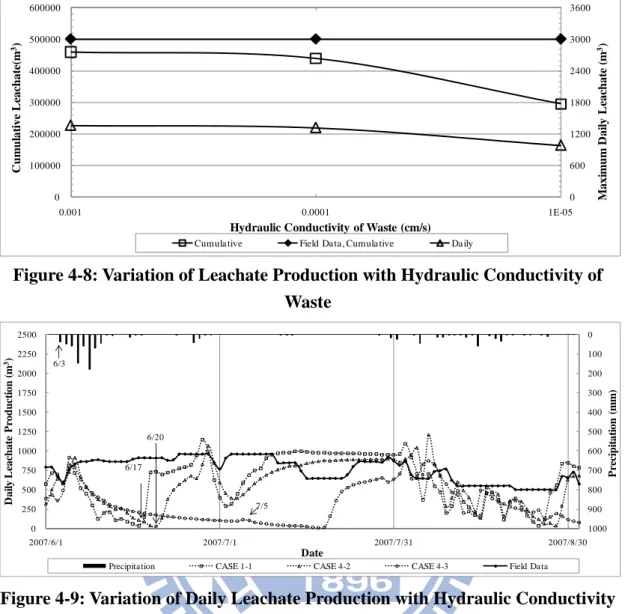
hydraulic Conductivity of LCRS ... 41 Figure 4-8: Variation of Leachate Production with Hydraulic Conductivity

of Waste ... 42 Figure 4-9: Variation of Daily Leachate Production with Hydraulic

Conductivity of Waste, between 2007/6/1 and 2007/9/1 ... 42 Figure 4-10: Variation of Loading Capacity with Days for Bali Landfill in

731 days ... 43 Figure 4-11: Cumulative Leachate Collection ... 45 Figure 4-12: Variation of Leachate Production with Evaporative Depth ... 46 Figure 4-13: Variation of Daily Leachate Production with Evaporative

Depth ... 46 Figure 4-14: Variation of Daily Leachate Production with Evaporative

Depth, between 2007/8/1 and 2007/12/31 ... 46 Figure 4-15: Variation of Leachate Production with LCRS Slope... 47 Figure 4-16: Variation of Leachate Production with LCRS Slope and the

(10)

IX

Figure 4-17: Variation of Leachate Head with LCRS Slope ... 48 Figure 4-18: Variation of Leachate Production and Leachate Head with

Hydraulic Conductivity of LCRS, Present... 49 Figure 4-19: Variation of Leachate Production and Leachate Head with

Hydraulic Conductivity of LCRS, Closed ... 50 Figure 4-20: Variation of Daily Leachate Production with Height of Waste,

Close Observation ... 50 Figure 4-21: Variation of Leachate Production with Hydraulic Conductivity

of Waste ... 50 Figure 4-22: Variation of Daily Leachate Production with Hydraulic

Conductivity of Waste, Close Observation ... 51 Figure 4-23: Variation of Loading Capacity with Days for Toufen Landfill

in 641 days ... 51 Figure 4-24: Cumulative Leachate Collection ... 54 Figure 4-25: Variation of Leachate Production with Evaporative Depth .... 54 Figure 4-26: Variation of Daily Leachate Production with Evaporative

Depth, between 2007/6/1 and 2007/9/1 ... 54 Figure 4-27: Variation of Leachate Production with Height of waste ... 56 Figure 4-28: Variation of Daily Leachate Production with Height of waste,

between 2007/5/20 and 2007/9/20 ... 56 Figure 4-29: Variation of Daily Leachate Head with Height of waste, Close

Observation ... 56 Figure 4-30: Variation of Daily Leachate Production with Height of waste

in 1994 ... 57 Figure 4-31: Variation of Leachate Head with Height of Waste in 1994 .... 57

(11)

X

Figure 4-32: Variation of Cumulative Leachate Production and Highest Leachate Head with the Height of Waste and Hydraulic Conductivity of LCRS ... 58 Figure 4-33: Leachate Production with Hydraulic Conductivity of Waste .. 59 Figure 4-34: Variation Daily Leachate Production with Hydraulic

Conductivity of Waste, between 2007/5/20 and 2007/9/20 ... 59 Figure 4-35: Variation Leachate Production and Leachate Head with

Hydraulic Conductivity of Waste, Closed ... 60 Figure 4-36 : Variation of Loading Capacity with Days for Anding Landfill

in 731 days ... 60 Figure 4-37: Variation Factor of Safety with Hydraulic Conductivity of

Leachate collection and removal system, with the interfacial friction angle as 15° ... 61 Figure 4-38: Variation Factor of Safety with Hydraulic Conductivity of

Leachate collection and removal system, with the interfacial friction angle as 8° ... 62 Figure 4-39: Variation Factor of Safety with Hydraulic Conductivity of

Leachate collection and removal system, Present ... 64 Figure 4-40: Variation Factor of Safety with Hydraulic Conductivity of

Leachate collection and removal system, Closed ... 64 Figure 4-41: Variation Factor of Safety with Hydraulic Conductivity of

Leachate collection and removal system, Present, Weak Interface Strength of GCL ... 64 Figure 4-42: Variation Factor of Safety with Hydraulic Conductivity of

(12)

XI

(13)

XII

Table List

Table 2-1: Summary of Landfill Failure (Qian and Koerner, 2005) ... 6

Table 2-2: Summary of HDPE/GCL Interfacial shear Strength (Triplett and Fox, 2001) ... 6

Table 2-3: Unit Weight and Strength Parameters of Municipal Solid Waste . 7 Table 2-4: Hydraulic Properties of Municipal Solid Waste ... 7

Table 3-1: Main Characteristic of Selected Landfill ... 18

Table 3-2: Summary of weather in Bali Landfill ... 22

Table 3-3: Summary of Weather in Toufen Landfill ... 25

Table 3-4: Summary of Climate in Anding ... 29

Table 3-5: Values of Cases for Sensitivity Analysis ... 31

Table 3-6: Result of Kmax ... 34

Table 3-7: Summary of Parameters for Slope Stability Analysis ... 35

Table 4-1: Summary of Simulation Result of Bali Landfill from HELP ... 36

Table 4-2: Summary of Simulation Result of Toufen Landfill from HELP 44 Table 4-3: Summary of Simulation Result of Anding Landfill from HELP 52 Table 4-4: Factor of Safety obtained from Slope Stability Analysis ... 62

Table 4-5 Summary of Safety of Factor obtained from Slope Stability Analysis in Toufen Landfill ... 65

(14)

1

Chapter 1 Introduction

1.1 Background

Due to the difficulty of obtaining land for disposing the municipal solid wastes or incinerator ash, many municipal solid waste landfills in Taiwan are located in mountain areas. Liner system is installed in the landfill to collect the leachate for treatment and prevent the leakage of leachate. Many reported slope failure of landfills have been associated with the excessive buildup of leachate level and excessive wetness of the geosynthetic interface, both of which is in turn related to clogging Leachate Collec-tion and Removal Systems (LCRS).

The buildup of leachate head in the landfill will cause the failure but the impor-tance of avoiding clogging of LCRS is sometimes ignored. Moreover, the leachate production rate and the ponding leachate head on the liner system is seldom moni-tored in Taiwan’s landfill. Moreover, due to the error design and lack of maintenance, some landfills have to face the problem of LCRS clogging. In Taiwan, the regulation does not emphasize on the design of LCRS hence the performance of LCRS is doubt-able. In addition, the design of LCRS does not fully employ the water balance simula-tion. Thus, the performance of LCRS should be examined and the design of LCRS should be improved.

1.2 Research Objectives

The objective of this study is to understand the performance of LCRS in various situations by simulating real landfills for water balance analysis and slope stability analysis. Three sites of landfill are located in the south, central, and north of Taiwan. They are chosen to be analyzed because of the different rainfall intensity, type of landform, and types of waste. In each landfill, different slope of LCRS and material

(15)

2

parameters are applied to water balance calculation. The results of leachate head are then used for slope stability analysis to study the consequential effect.

(16)

3

Chapter 2 Literature Review

2.1 Landfill Design and Operation

The major components of landfill are the liner system and the cover system. The liner system consists of LCRS and hydraulic barrier system. A typical profile of landfill is shown in Figure 2-1. The LCRS will drain the leachate out of the landfill to the wastewater treatment plant. The hydraulic barrier system will prevent leachate from infiltrating into the ground underneath the landfill. The gas produced by the waste will be collected with the gas collection system. When the waste reaches the designed vo-lume, the cover system will be constructed to reduce the generation of leachate and the landfill will be closed.

Figure 2-1: 3D Profile of the Landfill

2.2 Slope Stability Issue

Landfill is categorized into four types by the mode of fill, including area fill, trench fill, above and below ground fill, and valley fill (Qian et al., 2001). The waste in

Cover System

Leachate Collection and Removal System Barrier System

Gas Collection System

(17)

4

valley-filled landfill is piled from the bottom of landfill and the shape of the waste layer tends to be parallelogram as shown in Figure 2-2.

Figure 2-2: Profile of Valley-filled Landfill During Operation

The slope stability is critical to landfills in mountain areas. As indicated in Table 2-1, most landfills installed with liner system are involved with translational failure. The translational failure of landfill is due to two main mechanisms, including buildup of leachate head and wetting of interface in liner system (Qian and Koerner, 2005). The slip surface of translational failure lies along the liner system due to the low in-terfacial strength. Furthermore, absorption of leachate will cause of the increasing of unit weight of waste and thus will lower the stability of the waste (Koerner and Soong, 2000).

2.2.1 Interface Strength of Geosynthetics

There have been many studies on the interfacial shear strength between the geo-synthetics or between soil and geogeo-synthetics (Liu, 2004). In a series of shear strength test for interfaces of HDPE geomembrane and clay, the residual shear strength is about

Waste LCRS

Barrier System Slip Surface

(18)

5

43.1 kPa in submerged interface condition (Mitchell and Seed, 1990). The interfacial shear strength of HDPE geomembrane/compacted clay is between 11° and 14° while the clay is compacted to field density and water content. The unit weight of waste is17.3 kN/m3 and the height of overlying waste-fill is approximately 17.7 m, hence the residual friction angle can be determined as 8° (Seed and Mitchell, 1990). Some suggest that the friction angle of interface between geosynthestics should be as low as 8°. In the meantime, HDPE geomembrane and saturated compacted clay may be low while being in wet condition (Mitchell and Mitchell, 1992).

In the field test of slope stability for geosynthetic clay liner (GCL), the interface strength may be low since the bentonite inside the GCL tends to extrude through the opening of the geotextiles as GCL hydrates and thus reduce the interfacial shear strength (Daniel et al., 1998). The interfacial shear strength obtained from the labora-tory tests on the shear strength of the HDPE geomembrane and GCL interface are listed in Table 2-2 (Triplett and Fox, 2001). For smooth HDPE geomembrane/hydrated GCL interface, the residual cohesion is between 0.3 kPa and 5.8 kPa, and the friction angle is between 6.9° and 9.2°, respectively.

2.2.2 Properties of Municipal Solid Waste

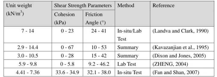
The unit weight and strength parameters of municipal solid waste (MSW) are listed in Table 2-3. The unit weight ranges from 2.9 kN/m3 to 14.4 kN/m3. For shear strength parameters, the cohesion ranges from 0 kPa to 67 kPa, and the friction angle covers from 9.2° to 53° due to the high heterogeneity of MSW.

The results of several researches on hydraulic properties of MSW are summa-rized in Table 2-4. The range of hydraulic conductivity of waste is from 4.0 10-2 cm/s to 4.2 10-5 cm/s.

(19)

6

Table 2-1: Summary of Landfill Failure (Qian and Koerner, 2005)

Case No

Type of Failure Reason for Low Initial FS

Triggering Mechanism

U-3 Translational Leachate Buildup Within Waste Mass

Excessive buildup of leachate level due to ponding

U-4 Excessive buildup of leachate level due to ice formation

L-4 Excessive buildup of leachate level due to liquid waste

L-5 Excessive buildup of leachate level due to leachate injection L-6 Excessive buildup of leachate level due to closed outlet valve L-7 Excessive buildup of leachate level due to leachate injection U-7 Single Rotational Excessive buildup of leachate level due to heavy rains

(hur-ricane) L-1 Translational Wet Clay Beneath

GM,i.e. GM/CCL composite

Excessive wetness of the GM/CCL interface

L-2 Excessive wetness of the GM/CCL interface

L-3 Excessive wetness of the bentonite in an unreinforced GCL

U-1 Single Rotational Wet Foundation or Soft Backfill Soil

Rapid rise in leachate level within the waste mass

U-5 Excessive buildup of perched leachate level on clay liner

U-6 Progressively weaker foundation soils

U-2 Multiple Rotational Foundation soil excavation exposing soft clay L: LINER

U: UNLINER

Table 2-2: Summary of HDPE/GCL Interfacial Shear Strength (Triplett and Fox, 2001)

GM/GCL Interface

Normal Stress range (kPa)

Peak Strengh Normal Stress range (kPa) Large Displacement (200 mm) Cohesion (kPa) Friction Angle (°) Cohesion (kPa) Friction Angle (°) SM/W 6.9-486 0.3 9.8 6.9-127 0.3 8.1 127-486 3.0 6.9 SM/NW 6.9-486 0.4 9.9 6.9-127 0.6 9.2 127-486 5.8 6.9 SM/W: 40 mil smooth HDPE / Woven geotextiles of woven/nonwoven needle-punched GCL

(20)

7

Table 2-3: Unit Weight and Strength Parameters of Municipal Solid Waste

Unit weight (kN/m3)

Shear Strength Parameters Method Reference Cohesion (kPa) Friction Angle (°) 7 - 14 0 - 23 24 - 41 In-situ/Lab Test

(Landva and Clark, 1990)

2.9 - 14.4 0 - 67 10 - 53 Summary (Kavazanjian et al., 1995) 3.0 - 10.5 0 - 28 15 - 42 Summary (Dixon and Jones, 2005)

5.9 - 9.8 0 - 5.8 9.2 - 46.2 Lab Test (ZHENG, 2004) 4.41 - 7.36 33.6 - 34.9 32.1 - 38.0 In-situ Test (Fan and Shan, 2007)

Table 2-4: Hydraulic Properties of Municipal Solid Waste

Hydraulic Conductivity (cm/s) Field Capacity (vol/vol) Wilting Point (vol/vol) Initial Water Content (%) Method Reference 1.0 10-2 - 1.0 10-4

5.8-9.2 8.55 - 20.5 Lysimeter (Fungaroli and Steiner, 1979)

4.0 10-2 - 1.0 10-3

Percolation

test in pits

(Landva and Clark, 1990)

1.0 10-3- 1.5 10-4

0.35 0.20 10 - 20 Pumping Test (Oweis et al., 1990)

0.12 0.11 18.4 - 6.7 ASTM 2325 (Benson and Wang, 1998) 1.1 10-3 -

2.9 10-4

0.36 0.17 39.0 Lab test (Jang et al., 2002)

2.3 Leachate Collection and Removal System 2.3.1 Design and Hydraulic Properties of LCRS

Leachate is generated from the initial water content of the waste, precipitation, and the degradation of wastes. In order to prevent the buildup of leachate head, LCRS is installed to collect the leachate from treatment. An LCRS is composed of a drainage blanket and a system of drainage pipes. Drainage pipes are placed in a fishbone pattern in the landfill and wrapped by gravel and geotextiles (Figure 2-3). The geotextiles is

(21)

8

used for protecting the drainage system from the clogging by the fines of waste or soil. The landfill which stores hazardous waste will have more than one leachate collection system. Therefore a secondary drainage layer will be installed underneath in order to detect the leakage of leachate.

Figure 2-3: Profile of Leachate Collection and Removal System

2.3.2 Design of LCRS

According to the regulation of landfill by of Taiwan (Department of Health, 1985), the basic liner system should consist of a drainage pipe with 1 m/s flow rate and a barrier with at least 10-6 cm/s of hydraulic conductivity. U.S Environmental Protec-tion Agency (USEPA) demands that the leachate head should be less than 30 cm (or 1 ft). In addition, there is no demand for specific flow rate of LCRS but the drainage layer shall be designed to reduce the leachate head on the liner system generated by the 24-hours, 2-year storm in 72 hours after the storm (USEPA, 1992).

For the prediction of leachate production in Taiwan, the rational method (Kuich-ling, 1889): Q= C·I·A ... (2.1) Coarse Sand Geomembrane Geotextile Gravel Drainage Pipe

(22)

9

is used, where Q is the peak discharge (m3); C is the runoff coefficient; I is the rainfall intensity (mm/hr); A is the drainage area (m2). Based on Equation 2.1, some equation for predicting leachate production is developed and applied (Wang, 2007). The mod-ified rational method (Foundation Conference on National Urban Cleaning, 1989): Q= (C1·A1+C2·A2)·I ... (2.2)

where the C1 is the runoff coefficient for the area of few-runoff and operation; C2 is

the runoff coefficient for the area of mass-runoff and closed area; A1 the area of

few-runoff and operation; A2 is the area of mass-runoff and closed area, is often used.

2.3.3 Clogging of Leachate Collection and Removal System

Researches indicate that the LCRS might clog in different situations. The majority of clogging of LCRS can be classified as three types: biological, physical, and chemical (Rowe and VanGulck, 2004). Field observations show that a thick slime layer was observed in the drainage blanket layer and the drainage pipe was clogged by the min-eral deposit (Fleming et al., 1999). In another field study, the hydraulic conductivity of sand was found to reduce from 4.3 10-2 cm/s to 1.6 10-5 cm/s because of the ce-menting within the void of the sand (Koerner and Koerner, 1995a).

The leachate of waste provides substance and nutrition for bacteria and hence the growing of biofilm inside the geotextiles induces the clogging (Mlynarek and Rollin, 1995). In laboratory tests on clogging by biofilm, the permeability of geotextiles was shown to decrease from 10-2 cm/s to 9.0 10-5 cm/s (Koerner and Koerner, 1995b) and 4 10-1 cm/s to 9 10-4 cm/s (Palmeira et al., 2008). On the other hand, the geotextiles soaked in the leachate are clogged by organic material and fine sediment. The per-meability of geotextiles was observed in the field and was found to decrease from 2.3 10-1 cm/s to 7.5 10-5 cm/s (Koerner and Koerner, 1995a).

(23)

10

2.4 Water Balance Calculation: Hydrologic Evaluation of Landfill Performance

Hydrologic Evaluation of Landfill Performance (HELP) is the most widely used computer program for water balance analysis of landfill (Albright et al., 2002; Nixon et al., 1997). HELP is developed by U.S. Army Engineer Waterways Experiment Sta-tion for the USEPA (Schroeder et al., 1994a). HELP is a quasi-two-dimensional hy-drologic model of water movement into or out from landfill, hence the calculation is one-dimensioned (Schroeder et al., 1994b). HELP have been used widely in the U.S.A for the design of landfill. In other countries, HELP was also employed in some studies and the results are fairly close to field data (Dho et al., 2002; Jang et al., 2002; Klaus, 2000).

2.4.1 Calculation Methods of HELP Model

The procedure of HELP can be described as six parts: weather input, and com-putation of runoff, potential evaporation, vertical drainage, lateral drainage, and geomembrane leakage (Schroeder et al., 1994b):

1. Weather Data: Weather data can be input by historical data or generated by weather generator. The weather data used in HELP includes precipitation, temperature, solar radiation, wind speed, and relative humidity.

2. Runoff Computation: SCS curve-number method is used for runoff. The ad-justment of curve number is related to the various levels of vegetation and the soil types in HELP model (USDA, 1985).

3. Evaporation Computation: The method follows the approach recommended by Ritchie (1972). Besides, a modified Penman (1963) equation

(24)

11

is used for soil water evaporation. This part contains potential evapotranspi-ration, surface evapoevapotranspi-ration, soil water evapoevapotranspi-ration, and plant transpiration. 4. Vertical Drainage Computation: The governing equation for vertical drainage

is Darcy’s law which will calculate the rate of vertical flow. In addition, Compell’s equation (1974),

K K SM RS_{UL RS} λ_{... (2.4)}

is applied to the unsaturated hydraulic conductivity.

5. Lateral Drainage Computation: The lateral drainage is considered as a flow in unconfined porous media and hence the Boussinesq equation (1904)

K_D h l sin α R, ... (2.5) is used for calculation. The percentage of lateral drainage is able to add to one layer for recirculation.

6. Geomembrane Leakage Computation: The calculation for leakage is based on Giroud and Bonaparte’s procedures. It will take area of defects, punctures, tears, cracks and seam situation into calculation (Giroud and Bonaparte, 1989).

2.4.2 Limitation of HELP

According to the researches on HELP, some limitations were mentioned. The parameters of surface and cover materials are found to affect the runoff, evapotrans-piration mostly. The under-predicted lateral drainage and runoff are due to the

over-estimation of the hydraulic conductivity of surface layers, which decrease the in-filtration of the precipitation. Moreover, the leachate production is under the influence of the evaporative depth. While the evaporative depth increases from 10 cm to 46 cm,

(25)

12

the leachate production decreases by more than 50% (Payton and Schroeder, 1988). In additional, HELP cannot calculate while the waste layer or LCRS degrades. Furthermore, HELP neglects the aging of cover system (Berger et al., 1996; Klaus, 2000). The HELP does not incorporate the degradation of specific layer, and should be supervised carefully during the construction. In this research, HELP is stated as simple because of the empirical modeling approach. In the other hand, there are more than a hundred empirical or theoretical equations for different situation and layer. Therefore, HELP is defined as very complex due to the different description of hy-drological process.

(26)

13

Chapter 3 Research Methodology

3.1 Structure of the Research Program

The structure of this study is shown in the flow chart in Figure 3-1. Visual HELP is developed for the Windows interface of HELP which was originally developed on DOS. Thus the latest version of Visual HELP is employed in this study.

Figure 3-1: Analysis flow chart

The weather data obtained from Central Weather Bureau is in the form of date-value which is unacceptable by Visual HELP. Hence, the weather data is trans-formed into Canadian Climate Centre format by Matlab®. The field data of leachate production, site plans, and design drawings are all obtained from the landfill operators and environmental protection bureaus of local governments. The landfills are divided

(27)

14

into zones according to different surface slope or drainage slope. In a landfill, profile is established for each zone and calculated in Visual HELP. A profile across the whole landfill is built for slope stability analysis. The result of lateral leachate drainage and leachate head will be analyzed for sensitivity of parameters and compared with field data. Then, the resulted leachate head will be applied to slope stability analysis by SLOPE/W.

3.2 Computer Programs 3.2.1 Visual HELP

The input of Visual HELP can be defined as three parts, the weather data, landfill profile, and material parameters. There are two ways to import weather data for Visual HELP, that is by generating synthetic weather data or inputting historic weather data. Visual HELP incorporates Weather Generator, which is developed by U.S Department of Agriculture (Richardson and Wright, 1984). There are two formats for inputting historic weather data. The first one of two types is Canadian Climate Centre format, which includes the data of precipitation, temperature, and solar radiation. The other one is National Oceanic and Atmospheric Administration format, which includes the data of precipitation, minimum temperature, and maximum temperature.

The weather data such as precipitation, temperature, and solar radiation are all transformed into Canadian Climate Centre format by Matlab®. Afterward, the trans-formed weather data will be input into Visual HELP.

The site parameters of landfill includes area, runoff area, initial surface water, and vegetation class for general settings and slope degree, slope length, surface slope, surface slope length, and thickness of each layer.

(28)

15

lateral drainage layer, barrier soil liner, geomembrane liner, and geotextiles and geonets. Moreover, there are default materials to build the profile of landfill. Except for geomembrane layer, six material parameters can be edited for the other layers, including total porosity, wilting point, saturated hydraulic conductivity, subsurface inflow, and initial moisture content. For the material parameters of geomembrane layer, there are pinhole density, installation defects, placement quality, and geotextile transmissivity for editing.

The flow chart for Visual HELP analysis is shown in Figure 3-2.

Historic Weather Data Characterization of Landfill Setup Profile of Landfill Establish Profile of Landfill Characterizati on of Landfill Weather Generator Data Output Water Balance Calculation

Synthetic Weather

Data Project Establish

Weather Data Input

(29)

16

3.2.2 SLOPE/W

Site Establishment for Analysis

Site profile is built by graphical user interface. The build of profile includes the geometry of the site, pore water pressure, external stress, anchor force, reinforcement, ground acceleration. The pore water pressure can be imported as pore water pressure ratio, Ru, and B-bar coefficients, or drawn as piezometric line and discrete points.

The parameters for building the profile for slope stability analysis include unit weight, cohesion, and internal friction angle.

Methods of Slope Stability Analysis

In this study, the failure surface of landfill is below the landfill and is irregular. Hence the calculation procedure by Morgenstern and Price are used. The failure sur-face is specified in the barrier layer since many failures occurred in the liner system. The procedure of slope stability analysis is shown in the flow chart in Figure 3-3.

(30)

17

Figure 3-3: Flow Chart of Slope Stability Analysis

3.3 Case Background

Three landfills, Bali Landfill, Toufen Landfill, and Anding Landfill, are selected in this study. The main characteristic of these three landfills are list in Table 3-1. These landfills are chosen from the northern, middle, and southern of Taiwan. Mean-while, the wastes in three landfills are all different from each other. Bali Landfill and Toufen Landfill are located in the valleys and hence the slope stability analysis will be applied on these two landfills. Anding Landfill is located in a plain so there is no ne-cessary to apply slope stability analysis on this landfill.

(31)

18

Table 3-1: Main Characteristic of Selected Landfill

Bali Landfill Toufen Landfill Anding Landfill

Location North of Taiwan Middle of Taiwan South of Taiwan

Landform Valley Valley Plain

Incoming Waste MSW MSW and

Incine-rator Fly Ash

Incinerator Fly Ash

Annual Precipitation (1989-2008)

2014 mm 1629 mm 1433 mm

3.3.1 Bali Landfill

Site Characteristic and Operation

Bali Landfill is located in a valley by the coast in northern Taiwan. The total area of Bali Landfill is 596,900 m2, which includes 118,626 m2 of area for the first 3 period of operation. The full site view is shown in Figure 3-4. The Bali Landfill has been in operation from 1997 till now. The operation of Bali landfill is divided into 4 periods, including 1st period, 2nd period, 3rd period, and post-3rd period. In the first 3 periods, only municipal solid waste was filled in the landfill and the incoming waste is 1,100 ton/day. The incinerator ash is only accepted by post-3rd period, and leachate drained from post-3rd period is separated for the other periods. Therefore, the post-3rd period is not included in this study.

(32)

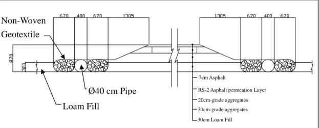
La Zon tile-incl in c V-sh base line pipe prof zon Figure 3 ndfill Desig Bali Land ne 1 has a ve -reinforced lines rapidly ontrast, the haped zone ed on the A According er system on es, loam fill file for HEL

e. The design Wastewater 3-4: Geogra gn dfill is divide ery steep slo wall. In com y. Zone 3 is feature of Z with flat su -A’ line in F g to the desi nly contains l, and a HDP LP. The heig ned maximu r Treatment aphy of Bal ed into 5 zo ope of botto mparison w disported du Zone 4 is th urface. The Figure 3-5.

ign data (Fig s a drainage PE geomem ght of waste um quantity t Plan 19 li Landfill, ones becaus om because with the othe

ue to the rap he relatively central prof gure 3-7) pr layer with mbrane layer e layer, slop y of daily le reprinted e of its irreg this zone is r 4 zones, th pidly rising y flat slope o file (Figure rovided from 400 mm-dia r for barrier pe degree, an eachate prod from Goog gular shape s facing the he surface s of the slope of bottom. Z 3-6) for slo m staff of B ameter HDP r. Figure 3-8 nd area diff duction trea 1st, 2nd, 3 Post 3 1st, 2nd, 3 Post 3 gle Earth (Figure 3-5 geotex-slope of zon e of bottom, Zone 5 is a ope stability Bali Landfill PE drainage 8 shows the fer from zon

atment is 80 3rd period 3rd period rd period 3rd period 5). ne 2 , and y is l, the e e ne to 0

(33)

20

m3 per day.

Figure 3-5: Bali Landfill from Plan View

Figure 3-6: Profile of Bali Landfill for Slope Stability Analysis

Zone 1 Zone 2 Zone 3 Zone 4 Zone 5 Present Boundary Elevation Contour Zone Boundary Central Profile Drainage Pipe A A’ Liner System

Top Boundary of Waste

Base Waste

(34)

21

Figure 3-7: Design Profile of Main Road and Drainage Pipe, Redraw from the Original Drawing

Climate

The weather data of Bali Landfill is obtained from Danshui Station. Considering the consistency of weather data, including daily precipitation, global solar radiation, daily temperature, quarterly relative humidity, and average wind speed, all weather data are selected from one weather station, No.466900 Danshui Station from 1989 to 2008.

The weather data of Bali Landfill is summarized in Table 3-2. The average an-nual precipitation is 2014 mm and the average anan-nual mean temperature is 22.1°C. The average relative humidity is 79%. Therefore, the climate in Bali can be defined as

Figure 3-8: Profile of Bali Landfill for HELP

Cover Soil Waste Layer Drainage Layer 2 mm HDPE GM Base Soil Non-Woven Geotextile Loam Fill Ø40 cm Pipe 7cm Asphalt

RS-2 Asphalt permeation Layer 20cm-grade aggregates 30cm-grade aggregates 30cm Loam Fill

(35)

“hum Ann Ann Rela 3.3. Sit Taiw Tou 29,3 Lan mid climate nual Precipi nual Mean T ative Humid .2 Toufen L e Characte Toufen La wan. Toufen ufen Landfil 360 m3 of cl ndfill accept Figure 3-9 Toufen L e”. Table 3-itation Temperature dity (quarte Landfill eristic and O andfill was l n Landfill n ll is 34,427 losed fill ar ts municipa 9: Geograp Landfill -2: Summa M 28 e 22 erly) 89 Operation located in a neighbors a c m3, which i rea. The clos

l solid wast phy of Touf Wa 22 ary of weath Maximum 865 mm 2.7 °C 9 % a valley near closed land includes 21 sed landfill tes, industria fen Landfil astewater Tr her in Bali Avera 2014 22.1 ° 79 % r Toufen To fill, (Figure ,618 m3 of t is not inclu al wastes, a ll, reprinted reatment Pl Clos Landfill age mm °C own, middle e 3-9). The t the present uded in this and incinera d from Goo an sed Landfill Minimum 968 mm 21.4 °C 74 % e region of total area of

fill area and study. Touf ator ash. ogle Earth l m f d fen

(36)

23

Landfill Operation and Design

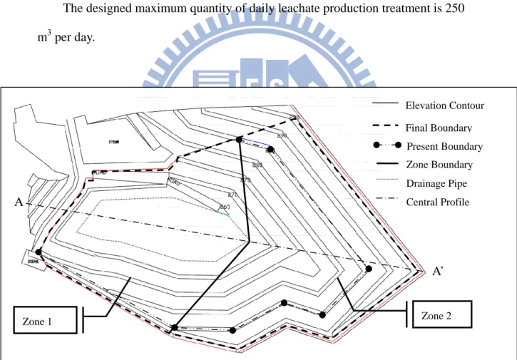
Toufen Landfill is divided into 2 zones, which is shown in Figure 3-10. Zone 1 has a flat slope of bottom, and Zone 2 has a much steeper slope than Zone 1 because Zone 2 includes most slope area of Toufen Landfill. The central profile of Toufen Landfill is shown in Figure 3-11, which is based on the A-A’ line in Figure 3-10.

The drainage layer is built with 600 mm-diameter HDPE pipes and loam fill. The barrier layer consists of a 2 mm thick HDPE geomembrane and a geosynthetic clay liner (GCL). The profile of Toufen Landfill is shown in Figure 3-12.

The designed maximum quantity of daily leachate production treatment is 250 m3 per day.

Figure 3-10: Toufen Landfill from Plan View, Redraw from the Origin Drawing

Present Boundary Elevation Contour Zone Boundary Central Profile Drainage Pipe Final Boundary Zone 1 Zone 2 A’ A

(37)

24

Figure 3-11: Profile of Toufen Landfill Side View

Climate

The nearest weather station Jhunan Station is at a distance of 4.85 kilometers from Toufen Landfill and is capable to provide daily precipitation, daily temperature, and average wind speed. Because global radiation and relative humidity are available from few weather stations, these two data are obtained from Hsinchu Station, which is 21.28

Figure 3-12: Profile of Toufen Landfill for HELP

Liner System

Liner System Top Boundary of Waste

Top Boundary of Waste

(a) Present (b) Final Cover Soil Waste Layer Drainage Layer 2 mm HDPE GM Base Soil GCL

(38)

25

kilometers away. The weather data were collected from 1993 to 2008.

The weather data of Toufen is summarized in Table 3-3. The average annual pre-cipitation is 1629 mm and the average annual mean temperature is 22.3°C. The aver-age relative humidity is 77%. Therefore, the climate of Toufen can be defined as “hu-mid climate”.

Table 3-3: Summary of Weather in Toufen Landfill

Maximum Average Minimum

Annual Precipitation 2192 mm 1629 mm 821 mm

Annual Mean Temperature 23.0 °C 22.3 °C 21.4 °C

Humidity (quarterly) 86 % 77 % 71 %

3.3.3 Tainan Anding Landfill

Site Characteristic and Operation

Tainan Anding Landfill is located in the middle of Tainan County, north of Tainan City. Anding Landfill is an above-ground-filled landfill, and the only source of waste is 180 ton/day incinerator ash from Yong-Kang Incinerator Plant. After being constructed in 2003, Anding Landfill has operated till now. Site view is shown in Figure 3-13. The present filled area of Anding Landfill is 27,086 m2. The subsidiary wastewater treat-ment plant treats not only the leachate from Anding Landfill, but also the leachate from the landfills of neighboring towns.

(39)

La line sand con a ba show A-A tion sign the pezi Figure 3-1 ndfill Desig According er system. T d and a barr sists of a dr arrier layer o wn in Figur A’ line in Fig n and the con ned fill limit

variation of The slope ium. Theref 13: Geograp gn g to the desi he primary rier layer of rainage laye of 1.5 mm H re 3-16. Fig gure 3-15. T ndition as r t is assumed f height of w of Anding fore, the lan

phy of And ign drawing liner system f 2 mm HDP er with HDP HDPE geom ure 3-17 ind The top bou reaching the d to include waste increa landfill is u ndfill is anal 26 ding Landfi g (Figure 3-1 m consists o PE geomem PE drainage membrane. T dicates the w undaries illu e level of de e two more l ases to 25.1 uniform and lyzed as a w Wastewa ill, reprinte 14), Anding of a drainag mbrane. The pipes and f The profile whole profi ustrate the ge esigned fill l levels for w m. d the shape o whole witho ater Treatme ed from Go g Landfill co e layer fille secondary filled with c of Anding L ile which is eometry of limit. In add water balanc of landfill is out subdivid ent Plant Anding L oogle Earth ontains a do ed with cour liner system course sand, Landfill is based on th present con dition, the d ce analysis w s similar to ded zones. Landfill h ouble rse m , and he ndi- de-with

(40)

tra-27

The designed maximum quantity of daily leachate production treatment is 600 m3 per day.

Figure 3-14: Detail of liner system of landfill

Figure 3-15: Anding Landfill from Plan View, Modified from the Original Drawing

Gas Pipe Concrete Base

Sand Bag

Gravel Fill Ø30 cm HDPE Drainage Pipe

30 cm Course Sand Fill 2.0 mm HDPE Geomembrane

30 cm Course Sand Fill 1.5 mm HDPE Geomembrane

Retaining Wall _Central

Drainage A

(41)

28

Figure 3-17: Profile of Anding Landfill Side View

Climate

The weather data is obtained from Tainan Station, which is 9.25 kilometers away from Anding Landfill. During 1998 to 2002, Tainan Station had been terminated and

Figure 3-16: Profile of Anding Landfill for HELP

Cover Soil Waste Layer Drainage Layer 2 mm HDPE GM Base Soil Drainage Layer 2 mm HDPE GM Liner System Top Boundary of Waste (close)

Top Boundary of Waste (present) Top Boundary of Waste (close

(42)

29

the meteorological observation had been changed to Yong-Kang Station which is 3.73 kilometers away from Anding Landfill. Hence the weather data is not entirely consis-tent due to the move of weather station.

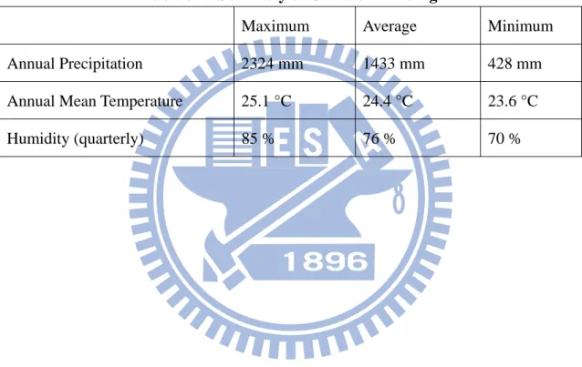
The weather data of Anding is summarized in Table 3-4. The average annual pre-cipitation is 1433 mm and the average annual mean temperature is 24.4°C. The aver-age relative humidity is 76%. Therefore, the climate of Toufen can be defined as “hu-mid climate”.

Table 3-4: Summary of Climate in Anding

Maximum Average Minimum

Annual Precipitation 2324 mm 1433 mm 428 mm

Annual Mean Temperature 25.1 °C 24.4 °C 23.6 °C

(43)

30

3.4 Study Scheme for Sensitivity Analysis

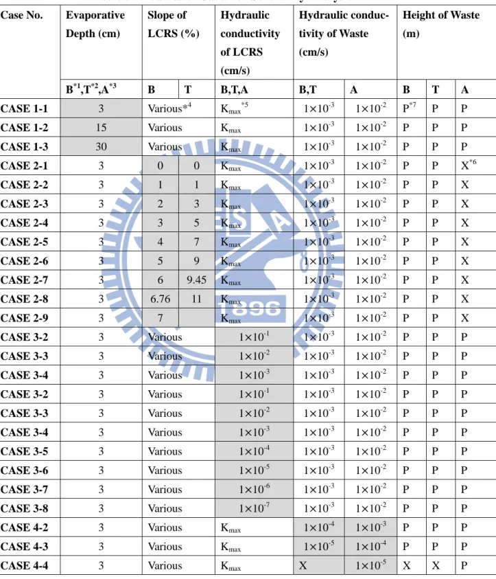
The sensitivity analysis is categorized into 8 cases as shown in Table 3-5. For CASE 1, CASE 2, CASE 3, CASE 4, and CASE 5, the evaporative depth, the slope of LCRS, the hydraulic conductivity of LCRS, the hydraulic conductivity of waste, and the height of waste is varied, respectively. Moreover, as the waste reaches the design fill limit, CASE 6 is varied for the slope of LCRS; CASE 7 and CASE 9 is varied for the hydraulic conductivity of LCRS. In this table, the background in the cells of varia-tion is filled with grey.

CASE 1-1 is defined as the initial case. In this case, hydraulic conductivities of waste and LCRS are representative of the most suitable condition of landfills in Taiwan. Furthermore, CASE 1-1 also equals to CASE 3-1, CASE 4-1, and CASE 5-1 because the parameters in CASE 1-1 are the initial value of evaporative depth, hydraulic con-ductivity of LCRS and waste, and height of the waste. Hence the series of CASE 3, CASE 4, and CASE 5 starts with CASE 1-1.

In the series of CASE 3, the average slope of LCRS will be applied in HELP. Anding Landfill is not included in this case due to its homogeneous slope (0.5%). From CASE 3-2 to CASE 3-8, the variation is the hydraulic conductivity of LCRS. The hydraulic conductivity of LCRS will be applied from Kmax to 1 10-7 cm/s. From

CASE 4-2 to CASE 4-5, the variation is the hydraulic conductivity of waste. From Case 5-1 to CASE 5-3, the variation is the height of the waste. This series of case is only applied for Toufen Landfill and Anding Landfill.

The series of CASE 6 and CASE 7 are all calculated as the waste layer reach the designed fill limit. In addition, the series of CASE 9 is calculated as the waste layer plus two more layer of waste. From CASE 6-2 to CASE 6-8, the variation is the slope of LCRS. The variation in series of CASE 7 and CASE 9 is the hydraulic conductivity

(44)

31

of LCRS. Bali Landfill is close to the design fill limit, thus the variation of height of waste will not apply in the simulation of Bali Landfill.

Table 3-5: Values of Cases for Sensitivity Analysis

Case No. Evaporative

Depth (cm) Slope of LCRS (%) Hydraulic conductivity of LCRS (cm/s) Hydraulic conduc-tivity of Waste (cm/s) Height of Waste (m) B*1,T*2,A*3 B T B,T,A B,T A B T A

CASE 1-1 3 Various*4 Kmax

*5

1 10-3 1 10-2 P*7 P P

CASE 1-2 15 Various Kmax 1 10

-3

1 10-2 P P P

-3 1 10-2 P P P CASE 2-1 3 0 0 Kmax 1 10-3 1 10-2 P P X*6 CASE 2-2 3 1 1 Kmax 1 10-3 1 10-2 P P X CASE 2-3 3 2 3 Kmax 1 10 -3 1 10-2 P P X CASE 2-4 3 3 5 Kmax 1 10 -3 1 10-2 P P X CASE 2-5 3 4 7 Kmax 1 10-3 1 10-2 P P X CASE 2-6 3 5 9 Kmax 1 10-3 1 10-2 P P X CASE 2-7 3 6 9.45 Kmax 1 10 -3 1 10-2 P P X CASE 2-8 3 6.76 11 Kmax 1 10 -3 1 10-2 P P X CASE 2-9 3 7 Kmax 1 10-3 1 10-2 P P X CASE 3-2 3 Various 1 10-1 1 10-3 1 10-2 P P P CASE 3-3 3 Various 1 10-2 1 10-3 1 10-2 P P P CASE 3-4 3 Various 1 10-3 1 10-3 1 10-2 P P P CASE 3-2 3 Various 1 10-1 1 10-3 1 10-2 P P P CASE 3-3 3 Various 1 10-2 1 10-3 1 10-2 P P P CASE 3-4 3 Various 1 10-3 1 10-3 1 10-2 P P P CASE 3-5 3 Various 1 10-4 1 10-3 1 10-2 P P P CASE 3-6 3 Various 1 10-5 1 10-3 1 10-2 P P P CASE 3-7 3 Various 1 10-6 1 10-3 1 10-2 P P P CASE 3-8 3 Various 1 10-7 1 10-3 1 10-2 P P P

-4

1 10-3 P P P

CASE 4-3 3 Various Kmax 1 10-5 1 10-4 P P P

(45)

32

Table 3-5: Values of Cases for Sensitivity Analysis (Continued)

Case No. Evaporative

Depth (cm) Slope of LCRS (%) Hydraulic conductivity of LCRS (cm/s) Hydraulic conduc-tivity of Waste (cm/s) Height of Waste (m) B*1,T*2,A*3 B T B,T,A B,T A B T A

CASE 5-2 3 Various Kmax 1 10-3 1 10-2 X X C

*8

-3 1 10-2 X X C+2*9 CASE 6-1 3 X 0 Kmax 1 10-3 1 10-2 X C X CASE 6-2 3 X 1 Kmax 1 10 -3 1 10-2 X C X CASE 6-3 3 X 3 Kmax 1 10 -3 1 10-2 X C X CASE 6-4 3 X 5 Kmax 1 10-3 1 10-2 X C X CASE 6-5 3 X 7 Kmax 1 10-3 1 10-2 X C X CASE 6-6 3 X 9 Kmax 1 10 -3 1 10-2 X C X CASE 6-7 3 X 9.45 Kmax 1 10 -3 1 10-2 X C X CASE 6-8 3 X 11 Kmax 1 10-3 1 10-2 X C X CASE 7-2 3 Various 1 10-1 1 10-3 1 10-2 X C C CASE 7-3 3 Various 1 10-2 1 10-3 1 10-2 X C C CASE 7-4 3 Various 1 10-3 1 10-3 1 10-2 X C C CASE 7-5 3 Various 1 10-4 1 10-3 1 10-2 X C C CASE 7-6 3 Various 1 10-5 1 10-3 1 10-2 X C C CASE 7-7 3 Various 1 10-6 1 10-3 1 10-2 X C C CASE 7-8 3 Various 1 10-7 1 10-3 1 10-2 X C C CASE 9-2 3 Various 1 10-1 X 1 10-2 X X C+2 CASE 9-3 3 Various 1 10-2 X 1 10-2 X X C+2 CASE 9-4 3 Various 1 10-3 X 1 10-2 X X C+2 CASE 9-5 3 Various 1 10-4 X 1 10-2 X X C+2 CASE 9-6 3 Various 1 10-5 X 1 10-2 X X C+2 CASE 9-7 3 Various 1 10-6 X 1 10-2 X X C+2 CASE 9-8 3 Various 1 10-7 X 1 10-2 X X C+2 *1: B = Bali Landfill *2: T = Toufen Landfill *3: A = Anding Landfill

*4: Various: slope of LCRS is different from zone to zone

*5: Kmax = max hydraulic conductivity of LCRS

*6: X = Not included in this case *7: P = Present Height;

*8: C = Closed (Reach designed fill limit) *9: C+2 = Closed with 2 more levels

(46)

33

The result of daily and cumulative leachate production will be compared to the field data. The difference between simulation and field data will be quantified by root mean square method. The difference will be calculated from the first date of the field data.

Since there is no research on hydraulic conductivity of waste in landfills in Taiwan, the hydraulic conductivity has to be adopted from foreign researches of landfills (Table 2-4). The hydraulic conductivity of waste layer is assumed to be 1 10-3 cm/s for MSW and 1 10-2 cm/s for incinerator fly ash. In order to obtain conservative results, the evaporative depth is set to be 3 cm in the initial condition for ensuring the maximum leachate collection.

Derivation of Kmax

The total quantity of leachate is Q and the hydraulic conductivity of drainage layer is Kmax. As shown in Figure 3-18, the drainage layer consists of the drainage pipe and

the loam material such as MSW hence the total quantity of leachate collection from drainage layer is also consisted from drainage pipe, Qpipe, and loam material, Qloam.

Since:

Qmax = Qpipe + Qloam, ... (3.1)

Kmax·i·Atotal=Kpipe·i·Apipe+Kloam·i·Aloam, ... (3.2)

where Kpipe=hydraulic conductivity of drainage pipe, which is assumed as 1 m/sec;

Apipe=area of drainage pipe; Kloam=hydraulic conductivity of loam material of the

drainage layer, such as MSW (K = 0.001 cm/s); Aloam=area of loam material of the

drainage layer. Atotal=Total area of the drainage layer, which is: Atotal= Apipe+ Aloam.

The hydraulic gradient, i, is constant in drainage layer and it is also the same value in the drainage pipe and loam material. Therefore, both i are all removed from the

(47)

34

equation and the equation shows:

K K _A A K _A A ... (3.3) The calculation result of Kmax for Bali Landfill, Toufen Landfill, and Anding

Landfill are listed in Table 3-6.

Table 3-6: Result of Kmax

Name Bali Landfill Toufen Landfill Anding Landfill

Width of Area 144 m 169 m 137 m

Diameter of Drainage Pipe 400 mm 600 mm 300 mm

Kmax (cm/s) 0.175 0.3345 0.679

To get conservative result, the runoff is assumed as zero and the vegetation class is set as bare soil. Above two parameters of HELP is in order to produce the maximum amount of leachate.

Slope Stability Analysis

The profile of landfill is divided into three layers, waste layer, barrier layer, and the base layer. The base material of the landfill is assumed as soft rock. The unit weight of the soft rock is 24 kN/m3. According to the strength of classification from ISRM

(ISRM, 1981), the uniaxial compressive strength of the extremely weak rock is 250 kPa to 1000 kPa. In this study, the undrained cohesion is 250 kPa for obtaining

conserva-Fill Material, such as MSW Drainage Pipe

(48)

35

tional result. The stability analysis only calculates the factor of safety for the transla-tional failure, thus the material strength of base soil does not affect the result of anal-ysis.

The assumption of unit weight and shear strength are based on the result of field study in Taiwan (Fan and Shan, 2007). The material properties of waste are 10 kN/m3 for unit weight, 35° for friction angle, and 34 kPa for cohesion which are conducted from in-situ direct shear tests in Jhunan Landfill and Hukou Landfill.

Based on the research on interface strength of geosythetics, the interfacial shear strength between HDPE and soil is assumed as 15° for friction angle (Liu, 2004) and 0 kPa for cohesion. In additional, the internal friction angle is assumed as 8° for the condition of wetting under the geomembrane. Though geomembrane is only 2 mm, the ground surface is not completely flat in the landfill. Therefore, the thickness of liner system is set as 0.1 m.

The parameters for slope stability analysis are summarized in Table 3-7

Table 3-7: Summary of Parameters for Slope Stability Analysis

Waste Layer Barrier Layer Base Layer

Unit Weight (kN/m3) 10 10 24

Cohesion (kPa) 34 0 250 (Su)

Friction Angle (°) 35 15

(49)

36

Chapter 4 Result and Discussion

4.1 Water Balance Analysis 4.1.1 Bali Landfill

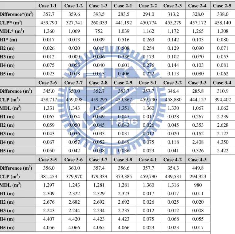
The summary of Visual HELP analysis for Bali Landfill is listed in Table 4-1.

Table 4-1: Summary of Simulation Result of Bali Landfill from HELP

Case 1-1 Case 1-2 Case 1-3 Case 2-1 Case 2-2 Case 2-3 Case 2-4 Case 2-5

Difference*(m3) 357.7 359.6 393.5 283.5 294.0 313.2 328.0 338.0 CLP* (m3) 459,790 327,741 260,033 441,192 450,774 455,279 457,172 458,140 MDL* (m3) 1,360 1,069 752 1,039 1,162 1,172 1,265 1,308 H1* (m) 0.017 0.013 0.009 0.516 0.263 0.142 0.103 0.080 H2 (m) 0.026 0.020 0.015 0.508 0.254 0.129 0.090 0.071 H3 (m) 0.012 0.009 0.006 0.336 0.173 0.102 0.070 0.053 H4 (m) 0.075 0.053 0.040 0.601 0.276 0.144 0.103 0.081 H5 (m) 0.023 0.018 0.013 0.406 0.222 0.113 0.080 0.062

Case 2-6 Case 2-7 Case 2-8 Case 2-9 Case 3-1 Case 3-2 Case 3-3 Case 3-4

Difference (m3) 345.0 350.0 352.7 353.7 357.7 346.4 285.8 310.9 CLP (m3) 458,717 459,098 459,295 459,367 459,790 458,880 444,127 394,402 MDL (m3) 1,331 1,343 1,349 1,351 1,360 1,330 1,067 1,062 H1 (m) 0.065 0.054 0.049 0.047 0.017 0.028 0.267 2.239 H2 (m) 0.059 0.050 0.045 0.043 0.026 0.045 0.353 2.628 H3 (m) 0.043 0.036 0.033 0.031 0.012 0.020 0.162 2.122 H4 (m) 0.067 0.057 0.052 0.049 0.075 0.118 2.408 4.350 H5 (m) 0.050 0.042 0.038 0.036 0.023 0.041 0.326 2.422

Case 3-5 Case 3-6 Case 3-7 Case 3-8 Case 4-1 Case 4-2 Case 4-3

Difference (m3) 356.0 360.0 357.4 356.6 357.7 354.3 449.8 CLP (m3) 381,453 379,970 379,339 379,385 459,790 439,531 294,923 MDL (m3) 1,297 1,243 1,281 1,281 1,360 1,316 980 H1 (m) 2.309 2.322 2.329 2.323 0.017 0.017 0.011 H2 (m) 2.676 2.682 2.692 2.692 0.026 0.025 0.020 H3 (m) 2.243 2.244 2.234 2.235 0.012 0.012 0.008 H4 (m) 4.407 4.420 4.423 4.423 0.075 0.068 0.055 H5 (m) 4.056 4.066 4.065 4.066 0.023 0.023 0.017

Difference: Calculated by root mean square method; CLP: Cumulative Leachate Production; MDL: Maximum Daily Leachate; H1: Highest Leachate Head in Zone 1, similar to H2, H3, etc.

(50)

37

Figure 4-1 shows the cumulative leachate production of the most suitable condi-tion and the field data. The cumulative leachate produccondi-tion from field data is 550,618 m3 and the cumulative leachate production of CASE 1-1 is 459,789 m3, which is the maximum among the cases and the closest to the field data. The difference is calcu-lated by root mean square method and the smallest one is 283.5 m3 which is obtained from CASE 2-1. It shows that the simulation of leachate production approaches the field data when the slope of LCRS is 0 %. Though the difference of CASE 2-1 is rela-tive small to the other cases, the leachate production is only 441,191 m3. Therefore, the difference is less in CASE 2-1 but the accumulative leachate production in CASE 1-1 is closer to the field data.

The variation of leachate production with the evaporative depth is shown in Fig-ure 4-2. It indicates that while the evaporative depth increases from 3 cm to 30 cm, the cumulative decreases from 459,790 m3 to 260,033 m3. The maximum daily leachate production decreases from 1,360 m3 to 752 m3 due to the increase of the evaporation. The daily leachate production is shown in Figure 4-3. Figure 4-4 provides a close ob-servation of daily leachate production between 2007/6/1 and 2007/9/1. It can be seen that though the evaporation increases, the time lag of leachate increases only within 4 days. The time lag of leachate production is similar with different evaporative depth hence the evaporation mainly affects the leachate production.

(51)

38

Figure 4-1: Cumulative Leachate Collection

Figure 4-2: Variation of Leachate Production with Evaporative Depth

Figure 4-3: Variation of Daily Leachate Production with Evaporative Depth

2007/1/1 2007/3/1 2007/5/1 2007/7/1 2007/9/1 2007/11/1 2008/1/1 2008/3/1 2008/5/1 2008/7/1 2008/9/1 2008/11/1 0 100 200 300 400 500 600 700 800 900 1000 0 50000 100000 150000 200000 250000 300000 350000 400000 450000 500000 550000 600000 P reci p it a ti o n ( m m ) C u mu la tiv e L ea ch a te P ro d u ctio n ( m 3) DATE

Precipita tion Field Da ta , Cumula tive CASE 1-1 CASE 2-1

0 600 1200 1800 2400 3000 3600 0 100000 200000 300000 400000 500000 600000 3 6 9 12 15 18 21 24 27 30 M a x imu m D a il y L ea ch a te (m 3) C u m u la ti ve L each a te ( m 3) Evaporative Depth (cm)

Cumula tive Field Da ta , Cumula tive Da ily

2007/1/1 2007/3/1 2007/5/1 2007/7/1 2007/9/1 2007/11/1 2008/1/1 2008/3/1 2008/5/1 2008/7/1 2008/9/1 2008/11/1 0 100 200 300 400 500 600 700 800 900 1000 0 250 500 750 1000 1250 1500 1750 2000 2250 2500 P reci p it a ti o n ( m m ) D ai ly L ea chat e P rodu ct ion ( m 3) DATE

(52)

39

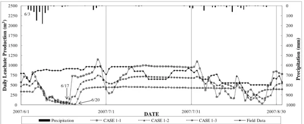
Figure 4-4: Variation of Daily Leachate Production with Evaporative Depth, be-tween 2007/6/1 and 2007/9/1

Figure 4-5 shows the result variation of leachate production with the slope of LCRS. Figure 4-6 shows the result of highest leachate head in each zone of Bali Landfill with the change of slope. The increase of leachate production and decrease of highest leachate head are due to the increase of slope of LCRS. The cumulative lea-chate production increases from 441,191 m3 to 459,367 m3 while the slope increases to 7%. In addition, the daily leachate production increases from 1,038 m3 to 1,349 m3 while the cumulative leachate production tends to be stable after slope is steeper than 4%. In each zone of Bali Landfill, the highest leachate head also tends to reach stable.

Figure 4-5: Variation of Leachate Production with LCRS Slope 6/3 6/17 6/20 0 100 200 300 400 500 600 700 800 900 1000 0 250 500 750 1000 1250 1500 1750 2000 2250 2500 2007/6/1 2007/7/1 2007/7/31 2007/8/30 P re cip it a ti o n ( m m ) D ai ly L ea chat e P rodu ct ion ( m 3) DATE

Precipita tion CASE 1-1 CASE 1-2 CASE 1-3 Field Da ta

0 600 1200 1800 2400 3000 3600 0 100000 200000 300000 400000 500000 600000 0 1 2 3 4 5 6 7 8 M axi m u m D a il y L eac hat e (m 3) C u m u la ti ve L eac ha te ( m 3)

Slope of Leachate Collection System (%)

(53)

40

Figure 4-6: Variation of Leachate Head with LCRS Slope

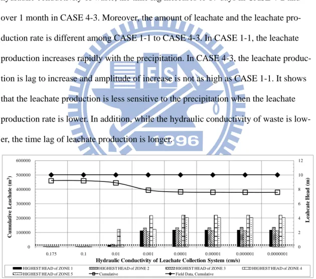
Figure 4-7 shows the variation of leachate production and highest leachate head with the hydraulic conductivity of LCRS. The cumulative leachate production reduces from 459,790 m3 to 379,385 m3 when the hydraulic conductivity of LCRS decreases from 0.175 cm/s to 1.0 10-4 cm/s. The reduction of leachate production approaches to about 379,000 m3 due to the calculation method of HELP. In HELP, the leachate pro-duction is governed by lateral drainage. Once the leachate head is higher than drai-nage layer, the draidrai-nage rate will include the layer above lateral draidrai-nage layer into calculation. In this study, the layer above LCRS is the waste layer. The hydraulic conductivity of waste layer is larger than the LCRS for more than 1 to 3 orders of magnitude when the hydraulic conductivity of LCRS is lower than 0.001 cm/s. Therefore, the flow rate is controlled by the hydraulic conductivity of waste layer when the leachate head is higher than LCRS.

Figure 4-8 shows the relation between leachate production and the hydraulic conductivity of waste. While the hydraulic conductivity of waste decreases by 2 or-ders of magnitude, the cumulative leachate production reduces from 459,790 m3 to 294,923 m3. The daily leachate production reduces from 1,360 m3 to 980 m3. The in-crease of hydraulic conductivity of waste causes the leachate head to rise. The evapo-ration does not increase with the decrease of flow rate hence there is no reduction for

0.0 0.2 0.4 0.6 0.8 1.0

Highest Hea d a t Zone 1 Highest Hea d a t Zone 2 Highest Hea d a t Zone 3 Highest Hea d a t Zone 4 Highest Hea d a t Zone 5

L eac hat e H ead (m ) CASE 1-1 CASE 2-1,slope=0% CASE 2-2,slope=1% CASE 2-3,slope=2% CASE 2-4,slope=3% CASE 2-5,slope=4% CASE 2-6,slope=5% CASE 2-7,slope=6% CASE 2-8,slope=6.76% CASE 2-9,slope=7%

(54)

41

the leachate produced by precipitation. Therefore, the increase of hydraulic conduc-tivity of waste causes the leachate head to rise.

As shown in Figure 4-9, the decrease of hydraulic conductivity of waste causes the increase of time lag of leachate production. In Figure 4-9, the hydraulic conduc-tivities of waste for CASE 1-1, CASE 4-2, CASE 4-3 are 1 10-3 cm/s, 1 10-4 cm/s, 1 10-5 cm/s, respectively. There is one rainfall started at 6/3. After 11 days, the de-creasing leachate production begins to increase in CASE 1-1. With the decrease of hydraulic conductivity of waste, the time lag increases to 17 days in CASE 4-2 and over 1 month in CASE 4-3. Moreover, the amount of leachate and the leachate pro-duction rate is different among CASE 1-1 to CASE 4-3. In CASE 1-1, the leachate production increases rapidly with the precipitation. In CASE 4-3, the leachate produc-tion is lag to increase and amplitude of increase is not as high as CASE 1-1. It shows that the leachate production is less sensitive to the precipitation when the leachate production rate is lower. In addition, while the hydraulic conductivity of waste is low-er, the time lag of leachate production is longer.

Figure 4-7: Variation of Leachate Production and Leachate Head with hydraulic Conductivity of LCRS 0 100000 200000 300000 400000 500000 600000 0 2 4 6 8 10 12 0.175 0.1 0.01 0.001 0.0001 0.00001 0.000001 0.0000001 C u m u la ti v e L ea ch a te (m 3) L eah cat e H ead ( m )

Hydraulic Conductivity of Leachate Collection System (cm/s)

HIGHEST HEAD of ZONE 1 HIGHEST HEAD of ZONE 2 HIGHEST HEAD of ZONE 3 HIGHEST HEAD of ZONE 4

(55)

42

Figure 4-8: Variation of Leachate Production with Hydraulic Conductivity of Waste

Figure 4-9: Variation of Daily Leachate Production with Hydraulic Conductivity of Waste, between 2007/6/1 and 2007/9/1

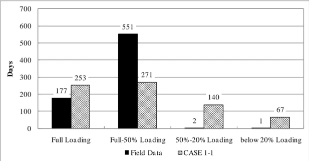
Figure 4-10 indicates the loading condition for daily leachate treatment. In 731 days, the loading capacity is above 50% for 728 days in field data and 524 days in CASE 1-1. The daily leachate treatment is in full loaded capacity for 174 days in field data and 253 days in CASE 1-1.

0 600 1200 1800 2400 3000 3600 0 100000 200000 300000 400000 500000 600000 1E-05 0.0001 0.001 M a xi m u m D a il y L eac ha te ( m 3) C u m u la ti ve L each a te (m 3)

Hydraulic Conductivity of Waste (cm/s)

Cumula tive Field Da ta , Cumula tive Da ily

6/3 6/17 6/20 7/5 0 100 200 300 400 500 600 700 800 900 1000 0 250 500 750 1000 1250 1500 1750 2000 2250 2500 2007/6/1 2007/7/1 2007/7/31 2007/8/30 P re ci p ita ti o n (mm) D a il y L eac h a te P rod uct ion (m 3) Date

(56)