時間區間事件之有效率的循序樣式探勘

(1)

時間區間事件之有效率的循序樣式探勘

研究生：姜季強指導教授：李素瑛

國立交通大學資訊科學與工程研究所

摘要

現在已經發展的循序樣式探勘演算法皆假設事件的發生是在時間點上。然而，在現實生活上發生的事件通常是持續一段時間的，稱之為“以時間區間為基礎的事件＂。但是由於時間區間事件間複雜的關係，造成了在設計有效率以時間區間事件為基礎之循序樣式探勘演算法上的困難。因此，我們提出了“同時發生的事件片段＂的概念來解決時間區間事件間複雜關係的問題。首先根據時間區間的事件間“同時發生＂的部份將時間區間事件切割成互斥的更小事件片段，即“同時發生＂的一段時間區間內可能有許多事件片段，而原本的事件序列可表示成我們所提出新的事件序列表示方式：以“同時發生＂時間排列的有序序列，稱之為“同時發生事件片段序列表示法＂。因此，我們考慮事件片段間的相互關係變地相當簡單，即前後、同時。我們提出一個演算法 CTMiner 基於“同時發生事件片段序列表示法＂來表示事件序列並利用知名的循序樣式探勘演算法 PrefixSpan 的概念來找出頻繁的時間區間事件循序樣式，並能完全避免產生候選樣式。最後，為了能理解頻繁的“同時發生事件片段序列＂樣式的意義，我們利用關係序列來呈現此頻繁樣式中時間區間事件間所有的關係。並且，我們還根據“同時發生的事件片段＂的特性，設計了一些策略來提升CTMiner演算法的效率。在實際的圖書館借閱資料和合成資料的實驗結果皆表現出此演算法的效率和適應性。

(2)

(3)

An efficient interval-based sequential pattern mining

Student:

Ji-Chiang

Jiang

Advisor:

Suh-Yin

Lee

Institute of Computer Science and Information Engineering

National Chiao-Tung University

Abstract

Existing sequential pattern mining algorithms assume that events occur instantaneously. However, events in real world applications usually have durations which are called interval-based events. But complex relationship among event intervals causes difficulty in designing an efficient interval-based event mining algorithm. Therefore, the concept of “coincidence-slice” is proposed to solve the problem caused by the complex relationship among event intervals. The event intervals are incised to disjoint smaller “event slices” according to the coincidences among event intervals, that is, several event slices may occur in the same time period called “coincidence”. Therefore, an original event sequence can be represented as a list of ordered “coincidences” which contains event slices. This new representation proposed is called “coincidence sequence representation”. We transform the problem of complex relationship among event interval to consider the simple relationship among event slices. The proposed interval-based sequential pattern mining algorithm called CTMiner is based on the “coincidence sequence representation”. The CTMier also uses the concept of well-known sequential pattern mining algorithm PrefixSpan to find temporal patterns without candidate generation. Finally, to comprehend the frequent temporal pattern represented by “coincidence sequence representation”, we discover and use relation list to present all the relationships in a pattern. We also implement some pruning strategies to improve the performance of CTMiner by considering the characteristics of the “Coincidence-slice”. Experiments on both synthetic datasets and real dataset of library

(4)

lending indicate the efficiency and scalability of the proposed algorithm.

(5)

Acknowledgement

I greatly appreciate the kind guidance of my advisor, Prof. Suh-Yin Lee. She not only helps with my research but also inspires and takes care of me. Without her graceful suggestion and encouragement, I cannot complete the thesis. Besides I want to give my thanks to all members in the Information System Laboratory for their suggestion and instruction, especially Mr. Yi-Cheng Chen, Miss Yu-Jiun Liu, Miss Chao-Ying Wu and Mr. Chang-Yei Pong. I would especially express my thanks to the nicest and most beautiful lady Miss Yi-chien Lee who accompanies me and lights up my life. Finally I would like to express my deepest appreciation to my parents. This thesis is dedicated to them.

(6)

List of Figures

Figure 2-1 Illustration for different representations of temporal pattern…….………..5 Figure 2-2 Two Ambiguity of representing temporal patterns in hierarchical

representation……….……….…………..6

Figure 3-1 All possible interval layouts between any consecutive time points.………..18 Figure 3-2 Illustration for occurrence numbers in event sequence and its corresponding

Csequence……….……….20

Figure 4-1 Illustration for merging event slice A+ and A- to form A and adjusting related

events………. ……….……….……….23

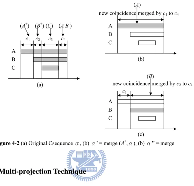
Figure 4-2 (a) Original Csequence α, (b) α’ = merge (A+,α), (b) α’’ = merge (B+,α)….25 Figure 4-3 Multi-projecting prefix 〈(A+)(B+)(C)〉 in (a) creates two postfix sequences (b) and

(c) to obtain complete frequent coincidence patterns…….………...27

Figure 5-1 The CTMiner algorithm. ……….………..30

Figure 5-2 The Incision_and_Projection algorithm. ……….……….31 Figure 5-3 Illustration for Incision_and_Projection on event sequence 3 in Table 3-1. The

cur_time_list and last_time_list point to the 6th and 5th time_list,

respectively. ……….…………33

Figure 5-4 The CPrefixSpan algorithm. ……….……….35

Figure 5-5 Illustrating three pruning strategies. ……….……….36 Figure 5-6 Illustration for elimination_test on A- successfully with all possible correlative

event slices in the prefix. ………...………..38

(9)

Figure 5-8 The Temporal_Relation_Discovery algorithm. ……….…………....43 Figure 5-9 Illustration for discovering temporal relations. (a) illustrates the Csequence and (b)

illustrates the relations determined by comparing the pseudo time points…………..……….…………....44

Figure 6-1 Performance of the four algorithms on data set with D10k – C10 – I1.25 – Ns

500 – Ni 2,500 – N10k………...………..47

Figure 6-2 The number of generated frequent pattern on dataset with D10k – C10 – I1.25 –

Ns 500 – Ni 2,500 – N1k..……….……….47

Figure 6-3 The distribution of frequent patterns of dataset with D10k – C20 – I2.5 – Ns 500 –

Ni 2,500 – N500……….………..48

500 – Ni 2,500 – N10k……….………..…49

Figure 6-5 The number of generated frequent patterns on dataset with D100k – C20 – I2.5 –

Ns 500 – Ni 2,500 – N10k.….…………..……..………49

Figure 6-6 The pattern length distribution of frequent patterns on dataset with D100k – C20 –

I2.5 – Ns 500 – Ni 2,500 – N10k..………….……….50

500 – Ni 2,500 – N10k……….………..51

Figure 6-8 The number of generated frequent pattern on dataset with D200k – C20 – I2.5– Ns

500 – Ni 2,500 – N10k……..……….………...51

Figure 6-9 The pattern length distribution of frequent patterns on dataset with D200k – C20 –

I2.5 – Ns 500 – Ni 2,500 – N10k.…..……….………52

Figure 6-10 Memory usage comparison of the four algorithms on data set with D100k –

C10 – I2.5 – Ns 500 – Ni 2,500 – N10k………53

Figure 6-11 Scalability test of the CTMiner algorithm with different database size and

minimum supports….………54

Figure 6-12 The number of generated frequent patterns with different database sizes and

minimum supports. ……….……….54

Figure 6-13 Experimental result of the CTMiner algorithm with varying minimum supports

(10)

Figure 6-14 The number of generated frequent patterns with varying minimum supports on

real dataset.……….………...………….……56

Figure 6-15 The pattern length distribution of pattern length of real dataset with varying

(11)

List of Tables

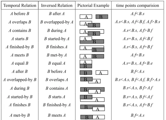
Table 1-1 The Allen’s 13 relations represent relations between any two event intervals. E.s

and E,f refer to start point and finish point of event E, respectively....……….3

Table 2-1 A sequence database……….………13

Table 2-2 Projected databases and sequential patterns……….………13

Table 3-1 Event sequences in the temporal database and its corresponding coincidence sequences. ……….………17

Table 3-2 Allen’s temporal relations map to coincidence representations...………20

Table 5-1 Original database……….……….40

Table 5-2 Projected databases and frequent temporal patterns……….………...…40

(12)

Chapter 1 Introduction

Sequential pattern mining is an active research topic in data mining domain in last decade, due to its widespread applicability including the analyses of customer purchase behavior, Web access patterns, scientific experiments, disease treatments, natural disasters, DNA sequences, and so on. The sequential pattern mining was first proposed by Agrawal and Srikant [1] and many studies have contributed to the efficient mining of sequential patterns. GSP [2], PSP [3], SPADE [4], PrefixSpan [5], and MEMISP [6] have focused on discovering frequent temporal patterns from instantaneous events, that is, events are treated as time points without duration. For example, consider a medical database, in which a patient's treatment is regarded each time as a time point-based event, indicating the time of the treatment, such as "cough→headache→fever". However, in many applications events are not instantaneous; they instead occur over a time interval. Time point-based sequential patterns are inadequate to express the complex temporal relationships in domains such as medical, multimedia, meteorology and finance where the duration of events provides more specific and richer information. Interval-based pattern (also called temporal pattern) mining is proposed focusing on the domains with interval data.

Mining patterns from interval data is undoubtedly more complex and arduous. It requires a different approach from mining patterns from time point-based data, such as mining traditional sequential patterns or episodes. So far, very little attention has been paid to the issue of mining time interval-based sequential pattern mining. To the best of our knowledge, the related researches in interval-based event mining are based on Allen’s temporal logics [7], which are categorized into 13 temporal relations between any two event intervals as: “before,” “after,” “overlap,” “overlapped-by,” “contain,” “during,” “start,” “started-by,” “finish,”

(13)

“finished-by,” “meet,” “met-by,” and “equal”. These 13 relationships can describe any relative position of two event intervals based on the arrangements of start points and finish points, as shown in Fig. 1-1. However, complex relationship among event intervals causes the difficulty while designing an efficient interval-based sequential pattern mining algorithm.

In this thesis, a new efficient algorithm called “CTMiner” (Coincidence Temporal pattern Miner) using the concept of the well-known sequential pattern mining algorithm PrefixSpan is proposed to discover temporal patterns from interval-based data without candidate generation. To address the problem of complex relationship among event intervals, a concept of coincidence-slice is developed. It focuses on coincidences among event intervals and incises the event intervals to disjoint smaller event slices according to coincidences then gathers the coincident event slices into the coincidence. Thus, the relationship among events is transformed to relationship among disjoint, smaller event slices and is simplified to “before”, “after” and “equal”. The event sequences are transformed to Coincidence sequences and thus facilitate the processing of interval-based pattern mining. Then the method called CPrefixSpan (Coincidence PrefixSpan) extends the concept of PrefixSpan to mine the frequent coincidence patterns. Due to the characteristic of coincidence-slice, the PrefixSpan is modified in order to cover all the frequent coincidence patterns. The multi-projection scheme is developed to obtain complete frequent coincidence patterns and three pruning strategies are also developed to improve the performance of our proposed algorithm. Finally, to comprehend a coincidence pattern, we use relation list to present all temporal relations in the coincidence pattern. Experimental studies on both synthetic and real datasets show that the proposed algorithm is efficient, scalable and outperforms the state-of-the-art algorithms.

(14)

Temporal Relation Inversed Relation Pictorial Example time points comparision

A before B B after A A.f<B.s

A overlaps B B overlapped-by A A.s<B.s, A.f<B.f, A.f>B.s

A contains B B during A A.s<B.s, A.f>B.f

A starts B B started-by A A.s=B.s, A.f<B.f

A finished-by B B finishes A A.s<B.s, A.f=B.f

A meets B B met-by A A.f=B.s

A equal B B equal A A.s=B.s, A.f=B.e

A after B B before A B.f<A.s

A overlapped-by B B overlaps A B.s<A.s, B.f<A.f, B.f>A.s

A during B B contains A B.s<A.s, B.f>A.f

A started-by B B starts A B.s=A.s, B.f<A.f

A finishes B B finished-by A B.s<A.s, A.f=B.f

A met-by B B meets A B.f=A.s

Table 1-1 The Allen’s 13 relations represent relations between any two event intervals. E.s

and E,f refer to start point and finish point of event E, respectively.

The rest of the thesis is organized as follows. Chapter 2 gives the motivation and related work. Chapter 3 provides the details of problem Definitions and the incision strategy. Chapter 4 describes the similarities and dissimilarities of projection scheme of PrefixSpan and CTMiner. Chapter 5 illustrates the CTMiner algorithm. Chapter 6 gives the experimental results and we conclude in Chapter 7. Note that, an event interval, i.e., interval-based event, in the rest of thesis is denoted as an event and instantaneous event is denoted as time point-based event. The start time point and finish time point of an event interval is denoted stp and ftp, respectively. A A A B A A A A A A A B B B B B B B B B B _A A B B A

(15)

Chapter 2 Motivation and Related Works

2.1 Motivation

2.1.1 Representations of a Temporal Pattern

Allen proposed 13 temporal relations between any two events without ambiguity. However, the representation of temporal patterns based on Allen’s logics will bear some problems as follows.

Various proposed representations suffer from different kinds of drawback.

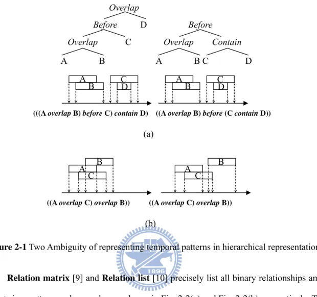
Hierarchical representation [8] describes relationships among more than three events

the which is a compact but lossy encoding method. There are two kinds of ambiguity problems in representation of a temporal pattern. First, the same relationship among events can be mapped to different temporal patterns. An example is shown in Fig. 2-1(a), in which a pattern can be expressed as “(((A overlap B) before C) contain D)” or “((A overlap B) before

(C contain D)).” Second, a temporal pattern can be represented as different relations among

events. For example, Fig. 2-1(b) shows that the pattern “((A overlap C) Overlap B))” can be represented in two different relations among events.

(16)

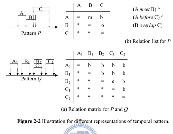
Figure 2-1 Two Ambiguity of representing temporal patterns in hierarchical representation. Relation matrix [9] and Relation list [10] precisely list all binary relationships among

events in a pattern, and examples are shown in Fig. 2-2(a) and Fig. 2-2(b), respectively. These unambiguous representations exhaustively list all (k×(k-1)/2) pairwise relations in a k-events

pattern, but it suffers from the problem of scalability in long temporal patterns. A

B C D A B C D

(((A overlap B) before C) contain D) ((A overlap B) before (C contain D))

A B A B C D

Overlap C Overlap Contain Before D Before

Overlap

(a)

((A overlap C) overlap B)) ((A overlap C) overlap B))

A A B B

C C

(17)

Temporal representation [11] utilizes time points arrangement to represent a temporal

pattern and sequence. For example, the pattern P shown in Fig. 2-2 can be represented in the unique expression “(A+<A-<B+<C+<B-<C-)”, where “ + ” or “ ¯ ” attached to an event indicates either a start time point or finish time point to the event, respectively. Due to the unique one-one mapping, it describes temporal pattern and sequence unambiguously.

TKSR (Time series Knowledge Representation) [12] expresses the temporal pattern

to the temporal concepts of coincidence with partial order. It describes a sequence of disjoint overlapped groups among events in order of time. In the same example as shown in Fig. 2-2, the pattern P can be represented as the expression “(A)(B)(BC)(C)” for coincidence order. The TKSR representation of pattern P and Q are the same because that TKSR does not specify overlap of an event to the other event is entire or part. Obviously, TKSR is not easily comprehensible and suffers the problem of ambiguity.

Augmented hierarchical representation [13] based on the hierarchical representation

solves ambiguity by attaching additional counting information to each hierarchy in

Figure 2-2 Illustration for different representations of temporal pattern.

(b) Relation list for P (A meet B) ^ (A before C) ^ (B overlap C) A C B Pattern P A B C A B C = m b * = o * * =

(a) Relation matrix for P and Q C1 Pattern Q A1 B1 B2 C2 A1 B1 B2 C1 C2 A1 B1 B2 C1 C2 = b b b b * = b b b * * = e b * * * = b * * * * =

(18)

chronological order. It has been proven that utilizing additional 5 counters i.e., contain,

finish-by, meet, overlap, start denoted as [c, f, m, o, s] to accumulate those 5 temporal

relations between the event e and all events occurring before e is sufficient to achieve an unambiguous representation. Take the pattern P in Fig. 2-2 as an example. First, we have “A meet B” so we set meet counter to 1 and it is represented as (A meet [00100] B). Then “B

overlap C” is attached to the expression and increments the length of the expression then

accumulates all 5 relations hence we set overlap and meet counter to 1. The pattern P can be expressed as “((A meet [00100] B) overlap [00110] C)”. The expression is not easily comprehensible and wastes (k-1)× 6 memory space in a k-events pattern.

2.1.2 The Problems of Complex relationship on Different Temporal Pattern

Mining Approaches

The relationships between two events in the temporal patterns are substantially

complex.

The relationship between any two time point-based events only indicates “before”, “after” and “equal” but there are Allen’s 13 temporal logics to represent the relationship among interval-based events due to the characteristic of time duration. Although the Allen’s 13 temporal logics can be normalized to 7 as the first 7 temporal relations shown in Fig. 1-1, i.e., “before”, “overlap”, “contain”, “start”, “finished-by”, “meet” and “equal”, by following the order of start time, finish time and event type. However, normalized Allen’s 7 temporal logics remain complex and cause the problem while applying it to different interval-based event mining approaches.

Generation-and-test approach [8, 9, 10, 12, 13]: It usually requires multiple iterations

to find all sequential patterns. In each iteration, some candidate patterns were generated and testified the frequency. Thus, reducing the number of candidate patterns is the main bottleneck

(19)

and challenge. The complicated relationships in interval-based event sequential pattern mining will lead to the generation of huge number of candidate patterns and bear tedious workload of support counting for candidate patterns.

Frequent Pattern-growth based approach [11, 14] is an efficient mining approach

which applies to time point-based patterns mining without candidate generation. It recursively partitions the time point-based event sequence database into smaller projected databases and grow the sequential patterns by exploring frequent time point-based events in associated projected database. The sequential pattern grows without candidate generation due to monotonic relationship between frequent 1-events and the corresponding prefix, i.e., only “before” and “equal”. A frequent 1-event can append directly to the prefix. To apply the approach to interval-based event pattern mining still requires candidate generation because of complicated relationship among events.

Based on the above observation, complex relationship is really a critical issue which causes prohibitively cost on time and space in mining processing. If the complicated relationship among events can be reduced in temporal pattern, then the efficient and effect of interval-based event mining algorithm will be improved substantially.

Related research themes of temporal pattern mining

A lot of extended researches [24, 25, 26, 27] of sequential pattern mining are very important and necessary, such as closed pattern mining, maximal patterns mining and incremental mining, sequential patterns classification, to name a few. Those researches developed based on time point-based event may not be suitable for interval-based event since the complex relationships among event intervals may degrade performance dramatically. To the best of our knowledge, there have been a few related researches about the extension of temporal pattern mining. Addressing the issue of complex relationship among events in temporal patterns provides us the opportunity for designing efficient related extensions of temporal pattern mining.

(20)

According to our observation, the different extent of overlap causes the complexity among events. Besides relation of “before” and “meet”, other five relations illustrate different extent of overlap. For instance, the “overlap” relation shows the overlapping on the front part and rear part of two events. Different correlated positions of an event which is fully overlapped by another event forms different relations, i.e., “start”, “contain”, “finished-by” or “equal”. Therefore, we classify different parts of event as event slices into overlap or non-overlap. Then, the relationship between event slices is very simple, i.e., “before”, “equal”. In general, event sequence also exhibits many overlaps among events. Therefore, in this paper, the concept of coincidence-slice and incision strategy is proposed which transform events of event sequence to event slices. The complex relationship among events is transformed to simpler relationship among event slices. The proposed concept of coincidence-slice and incision strategy is described in details in Chapter 3.

2.2 Related Works

Some recent researches have investigated the mining of sequential patterns with interval-based events [8, 9, 10, 11, 12, 13, 14]. Kam et al. [8] designed an Apriori-based algorithm that uses the hierarchical representation to discover frequent temporal patterns. The representation only keeps (k-1) relations and two time points of earliest and latest time points in a k-pattern. Therefore, the hierarchical representation is ambiguous and many spurious patterns are generated. Hoppner [9] also proposed an Apriori-based algorithm that counts support of all candidate patterns of length k by scanning database once with a sliding window. It also defined the supporting level of a pattern as the total time in which the pattern can be observed in a sliding window to improve the performance of the algorithm. However, a major concern for this approach is how to decide the proper size of the sliding window, since the

(21)

sliding window directly dominates the mining results and efficiency of the algorithm. It also needs to scan database repeatedly. Mochen [12] proposed a new representation, called TKSR, which uses the coincidence concept to facilitate the process of temporal patterns discovery. An event sequence can be treated as a series of disjoint overlaps named “coincidences”. It treats coincidence and event as itemset and item. Then it adopted CHARM [15] to find frequent itemsets as marginal-closed coincidences then applied the CloSpan [16] to mine the closed sequential patterns as partial ordering marginal-closed coincidences. The pattern represented with TKSR is ambiguous and is not easily comprehensible. Edi et al. [14] developed a pattern-growth algorithm, named ARMADA based on an efficient sequential patter mining algorithm MEMISP to find frequent temporal patterns and also reduces the memory space of projected databases. However, it still uses lots of memory space because temporal patterns are expressed by relation matrix. It requires only two database scans but it also generates a lot of candidates and accesses memory frequently due to complex relationship among events. Papapetrou et al. [10] proposed the Hybrid-DFS algorithm which is Apriori-based approach to mine temporal arrangements of temporal intervals and a relation list to express temporal patterns. It also proposed an enumeration tree structure to improve the performance of the algorithm. First, it scans database twice to obtain frequent 1-patterns and all related records of frequent 2-patterns as first and second levels of the tree respectively by BFS traverse order. To obtain the frequent k-patterns in the level k of the tree, it firstly merges frequent (k-1)-patterns and frequent 1-patterns in level (k-1) and 1, respectively. Because the k-patterns can be treated as the combination of frequent 2-patterns, so it scans related records in level 2 to verify the frequency of a specific k-pattern by DFS traverse order. It transforms an event sequence into a vertical representation using id-lists. The id-list of an event is merged with the id-list of other events to generate temporal patterns. This approach does not scale well when the length of temporal pattern increases. Wu et al. [11] derived a pattern-growth based algorithm called TprefixSpan for mining temporal pattern from interval-based events

(22)

and represents temporal patterns in compact but ambiguous temporal representation. It first discovers single frequent events from the projected database. Next, all the possible candidates could be generated while appending a discovered frequent 1-event to the prefix and all the possible relations between them need to be considered. Last, it scans the projected database again for support counting. TPrefixSpan still needs to scan the projected database multiple times and it does not employ any pruning strategy to reduce the search space. Patrel et al. [13] proposed an Apriori-based algorithm named IEMiner. It utilizes the additional counting information to achieve lossless hierarchical representation called augmented representation and generates frequent temporal patterns iteratively and increases the pattern length by one after iteration. It also proposed a support counting method to scan database once to derive the frequency of all candidate patterns in each iteration. When scans the database, many temporal patterns are generated by composing the events in database. If a generated pattern is a candidate pattern then we accumulate the support of the candidate pattern. After scanning, the frequency of candidate patterns is determined. The operation is very costly due to the complexity of augmented representation.

2.2.1 Sequential Pattern Mining Algorithm: PrefixSpan

We use the concept of the well-known pattern-growth based sequential pattern mining algorithm called PrefixSpan (i.e., Prefix-projected Sequential pattern mining), which explores prefix-projection in sequential pattern mining. For the sequential database S in Table 2-1 with minimum support = 2, sequential patterns in S can be mined by a prefix-projection method in the following steps.

Step 1: Find length-1 sequential patterns. Scan S once to find all frequent items in

sequences. Each of these frequent items is a length-1 sequential pattern. They are 〈A〉: 4, 〈B〉: 4, 〈C〉: 4, 〈D〉: 3, 〈E〉: 3 and 〈F〉: 3, where 〈pattern〉: count indicates the pattern and its

(23)

associated support count.

Step 2: Append each frequent 1-item to the prefix and create projected database with respect to the appended prefix. For the first time to append each frequent 1-item to the

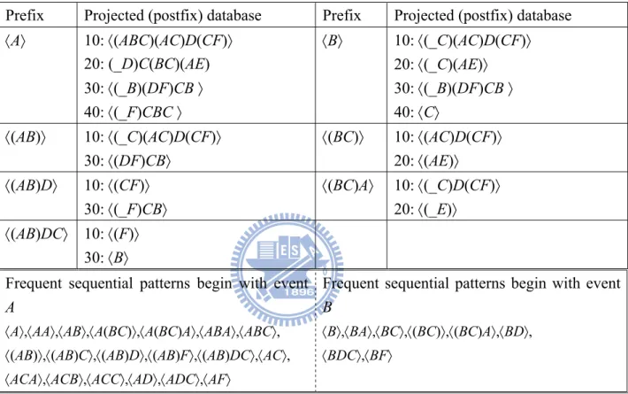
prefix, we directly set each frequent 1-item as appended prefix. And the complete frequent sequential patterns can be partitioned into |L1| parts, where |L1| is the number of frequent 1-items. Therefore, we have six projected databases with respect to the appended prefix, i.e., 〈A〉, 〈B〉,…, and 〈F〉. The projected databases with respect to prefixes 〈A〉 and 〈B〉 are shown in the 2nd row of Table 2-2, respectively.

Step 3: Recursively go back to step 1 to find whole frequent sequential patterns. For the

running example above, the frequent length-1 item of projected database with respect to prefix 〈A〉 are 〈B〉: 4, 〈_B〉: 2, 〈C〉: 4, 〈D〉: 2, 〈F〉: 2, where 〈_B〉 indicates item B occurs simultaneously with the items of last itemset in the prefix. After appending each frequent length-1 item to the prefix, the projected database of appending 〈_B〉 to the prefix 〈A〉 to form a new prefix 〈(AB)〉 is shown in 3rd row of Table 2-2. Similarly, the complete frequent sequential patterns begin with item A are generated and are shown in the last row of Table 2-2 if we keep going on the process.

(24)

Sequence_id Sequence

10 〈A(ABC)(AC)D(CF)〉

20 〈(AD)C(BC)(AE)〉

30 〈(EF)(AB)(DF)CB〉

40 〈 EG(AF)CBC 〉

Table 2-1 A sequence database

Prefix Projected (postfix) database Prefix Projected (postfix) database 〈A〉 10: 〈(ABC)(AC)D(CF)〉 20: (_D)C(BC)(AE) 30: 〈(_B)(DF)CB 〉 40: 〈(_F)CBC 〉 〈B〉 10: 〈(_C)(AC)D(CF)〉 20: 〈(_C)(AE)〉 30: 〈(_B)(DF)CB 〉 40: 〈C〉 〈(AB)〉 10: 〈(_C)(AC)D(CF)〉 30: 〈(DF)CB〉 〈(BC)〉 10: 〈(AC)D(CF)〉 20: 〈(AE)〉 〈(AB)D〉 10: 〈(CF)〉 30: 〈(_F)CB〉 〈(BC)A〉 10: 〈(_C)D(CF)〉 20: 〈(_E)〉 〈(AB)DC〉 10: 〈(F)〉 30: 〈B〉

Frequent sequential patterns begin with event

A

〈A〉,〈AA〉,〈AB〉,〈A(BC)〉,〈A(BC)A〉,〈ABA〉,〈ABC〉, 〈(AB)〉,〈(AB)C〉,〈(AB)D〉,〈(AB)F〉,〈(AB)DC〉,〈AC〉, 〈ACA〉,〈ACB〉,〈ACC〉,〈AD〉,〈ADC〉,〈AF〉

Frequent sequential patterns begin with event

B

〈B〉,〈BA〉,〈BC〉,〈(BC)〉,〈(BC)A〉,〈BD〉, 〈BDC〉,〈BF〉

(25)

Chapter 3 Problem Definitions and Incision Strategy

We focused on the discussion of temporal pattern mining due to the widespread applicability and lacking of researches. In this chapter, we define the problem of temporal pattern mining and introduce the incision strategy. The interval-based mining problem is much more arduous than traditional time point-based mining problem. Since relationship among events are more complicated than that of the time point-based events. The complex relation between two events is the major bottleneck for mining temporal pattern. Therefore, the incision strategy is proposed to transform event sequence to Coincidence sequence which addresses the critical issue of temporal pattern mining.

Definition 1 (Event interval) Let E = {e1, e2,…, ek} be a set of all event types. Without loss of generality, we define a set of uniformly spaced time points based on the real number R. We say the triplet (ei, si, fi) ∈ E × R × R is an event interval or temporal interval, where ei ∈ E, si, fi ∈ R and si < fi. The two time points si and fi are called start time point and finish time point and denoted as stp and ftp, respectively. The set of all event intervals over E is denoted by I. We write (e, s, f) ⊆ (e’, s’, f’) if s ≤ s’, f’ ≤ f.

Definition 2 (Event sequence and maximal property) An event sequence ei ∈ E is a series of event interval triplets 〈(e1, s1, f1), (e2, s2, f2), …, (em, sn, fn)〉, where m ≤ n since an event may occurs many times, si ≤ si+1, and si < fi ∀i. Every interval (ei, si, fi) must be maximal in sequence, i.e., there is no (ei, sj, fj) in the sequence such that neither sj nor fj occurs in the interval [si, fi]. We call this assumption, maximal property, defined as follows:

∀ ( ep, si, fi ), ( eq, sj, fj ) ∈ I, ( ep, si, fi ) ≠ ( eq, sj, fj ): si≤ sj∧ fi≥ sj ∧ ep≠ eq －(1) Equation (1) above is also called the maximality assumption [15]. The maximal property guarantees that each event interval is maximal in the series. If maximal property is violated, we can merge both event intervals and replace them by their union (ei, min(si, sj), max(fi, fj)).

(26)

Definition 3 (Temporal database) Considering a database D = {r1, r2, …, rm}, each record ri, where 1 ≤ i ≤ m, consists of a sequence-id and an event interval (ei , si , fi). Given a sequence set {q1, q2, …, qn}, each sequence qj is an event sequence with grouping the records in D with same sequence-id. D = {q1, q2, …, qn} is called a temporal database.

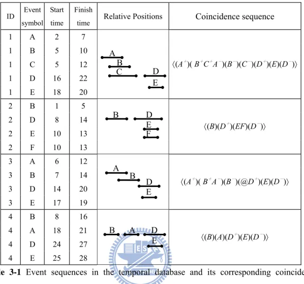
Actually, all events can be grouped together by the same sequence-id and arranged by non-decreasing order of start time, end time and event type into an event sequence. As the result, the database D can be viewed as a collection of event sequences. For example, in Table 3-1, the temporal database consists of 17 events, and 4 event sequences. We use normalized Allen’s 7 interval logics to describe the temporal relation between every two events in a sequence.

Definition 4 (Temporal pattern) Given n events (ei, si, fi), 1 ≤ i ≤ n, a temporal pattern of size n > 1 is defined as a matrix M ∈ An × n_{where A is a set of Allen’s temporal relations and} each index i maps to the corresponding event ei, the element M[i, j] denotes the relationship between two event intervals (ei, si, fi) and (ej, sj, fj). The number of intervals in the temporal pattern P is called the dimension of P, denoted as dim(P). If dim(P) = k, then P is called a

k-pattern.

Various representations have been proposed for temporal pattern, as we mentioned above. We adopt relation list to represent temporal pattern since it can precisely and unambiguously list all pairwise relationships among events in a pattern.

3.1 Incision Strategy

The coincidence-slice architecture is implemented by incision strategy. The proposed strategy cuts events into disjoint smaller event slices based on the global information of event sequence, i.e., time points of events, and the simultaneous event slices are collected into a

(27)

group called coincidence. We define event slice and coincidence as follows.

Definition 5 (Coincidence, Event time set and Event slice) Given an event sequence q =

〈(e1, s1, f1), (e2, s2, f2), …, (en, sn, fn)〉, A set T ={t1, t2 …tm-1, tm} ,where ti ∈ {s1, f1, s2, f2,…, sn, fn} , ti ≠ ti+1, and ti < ti+1 for 1 ≤ i < m without repetition, is called an event time set which collects all time points of event intervals with no repeat and in increasing order of time in q. A coincidence of q is a time period denoted as ci = (ti, ti+1) where ti, ti+1 ∈ T and 1≤ i<m. Therefore, we have (m-1) successive coincidences c1,c2,…,cm-1 in q. Furthermore, four types of event slices are defined as follows.

1. Start slice: A start slice of event ei in q is defined as an interval which belongs to coincidence ci and denoted as ei＋

if and only if (1) ti = si and(2) ti+1 < fi.

2. Finish slice: A finish slice of event ei in q is defined as an interval which belongs to coincidence ci and denoted as ei－

if and only (1) ti+1 = fi and (2) ti > si.

3. Intermediate slice: An intermediate slice of event ei in q is defined as an interval which belongs to coincidence ci and denoted as ei*_{if and only if (1) t}

i > si and (2) ti+1 < fi.

4. Intact slice: An intact slice of event ei in q is defined as an interval which belongs to coincidence ci and denoted as ei if and only if (1) ti = si, (2) ti+1 = fi.

For example, in Table 3-1, sequence 2 has 4 events: (B, 1, 5), (D, 8, 14), (E, 10, 13), (F, 10, 13) and its corresponding event time set = {1, 5, 8, 10, 13, 14}. There are five successive coincidences c1=(1,5), c2=(5,8), c3=(8,10), c4(10,13) and c5=(13,14). Hence the event D have three event slices: 1. start slice D＋

= (D, c3), 2. intermediate slice D* = (D, c4) and 3. finish slice D－

= (D, c5). The only event slice of event B is B = (B, c1). Obviously, an event can only have a pair of start slice and finish slice or one intact slice but it could have many intermediate slices. Actually, intermediate slices do not help in the mining processing due to a pair of start slice and finish slice or an intact slice is sufficient to imply the relative time positions of an event in an event sequence.

(28)

ID Event symbol

Start time

Finish

time Relative Positions Coincidence sequence

1 A 2 7 1 B 5 10 1 C 5 12 1 D 16 22 1 E 18 20 〈(A＋_{)( B}＋_C＋_A－_)(B－_)(C－_)(D＋_)(E)(D－_)〉 2 B 1 5 2 D 8 14 2 E 10 13 2 F 10 13 〈(B)(D＋ )(EF)(D－_)〉 3 A 6 12 3 B 7 14 3 D 14 20 3 E 17 19 〈(A＋_{)( B}＋_A－_)(B－_)(@D＋_)(E)(D－_)〉 4 B 8 16 4 A 18 21 4 D 24 27 4 E 25 28 〈(B)(A)(D＋ )(E)(D－_)〉

Table 3-1 Event sequences in the temporal database and its corresponding coincidence

sequences.

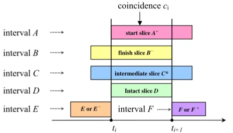
We obviously perceive that both event interval and event slice are composed of two time points of events in an event sequence. There are 4 kinds of event slices in two consecutive time points in an event sequence, as shown in Fig. 3-1. We only consider the period time between ti and ti+1, i.e., the coincidence ci. The event intervals finished at ti or started at ti+1 are not processed since we handle them in ci-1 = (ti－1, t_i) and ci+1 = (t_i+1, t_i+2),

respectively. For instance, in Fig. 3-1, events E and F are processed in ci-1 and ci+1, respectively. A start slice A+ in ci indicates that event A starts at ti and finishes after at ti+1 and a finish slice B- in ci indicates that event B starts before ti and finishes at ti+1. An intermediate slice C* in ci means that event C occurs across ci and an intact slice D in ci means that the duration of event D equals ci. The relationship between any two event slices can only be

A B C D E B D E F A B D E A B D E

(29)

“before”, “after” and “equal”. The relation between two event slices in the same period is “equal” and the relation between event slices in different periods is either “before” or “after”.

Definition 6 (Coincidence sequence with respect to an event sequence) A Coincidence

sequence denoted as Csequence consists of an ordered set of event slices and meet tokens

represent an event sequence unambiguously. Given an event sequence q = 〈(e1, s1, f1), (e2, s2,

f2), …, (en, sn, fn)〉, an event time set {t1, t2 …tm-1, tm} of q is created. Totally (m-1) continuous

coincidences c1,c2,…,ci,…,cm-1 are created. The event sequence q is transformed to Csequence by the incision strategy. The incision strategy transforms an event sequence q to coincidence sequence by the following operations.

1. Transforms event intervals to event slices

¾ An event occurs exactly at coincidence ci then the corresponding intact slice is created and is put into ci.

¾ An event occurs from ti to tj, where ti < tj and ti is the start time of cp and tj is the finish time of cq, then its corresponding start slice and finish slice are created and are put into cp and cq, respectively.

2. Place meet token to distinguish adjacent event intervals

¾ If there are two events (ei, si, fi) and (ei, sj, fj) meets at time t, i.e., t = fi = sj, and t is the finish time of cp and the start time of cp+1 then a meet token “@” is put into cp+1.

interval E interval C interval B interval A interval D intermediate slice C* start slice A+ E or E－ finish slice B－ ti ti+1 Intact slice D F or F+ interval F

Figure 3-1 All possible interval layouts between two consecutive end time points.

(30)

3. Finally, empty coincidences are removed and the remaining ordered coincidences form the Csequence.

Note that, event slices in coincidence are ordered by (1.) Intact slice (2.) Start slice (3.) Finish slice and event slices with the same type of event slice are ordered by event type.

We decide to remove all empty coincidences to save memory space. For instance, consider the sequence 4 in Table 3-1, There are two empty coincidences in the sequence which is represented as coincidence representation, i.e., 〈(B)( )(A)( )(D＋_)(E)(D－_)〉._{Although the}

incision strategy looks promising, actually it has a fatal defect. We cannot distinguish between two adjacent intervals and two separate intervals due to empty coincidence elimination. A meet token “@” is used to address this drawback. For example, there are two event sequences “A before B” and “A meet B” with the same coincidence representation 〈(A)(B)〉 by applying the incision strategy. A meet token “@” is placed in the coincidence ci+1 of Csequence of “ A meet B” where event A finished at ci which met event B started at ci+1, denote as 〈(A)(@B)〉.

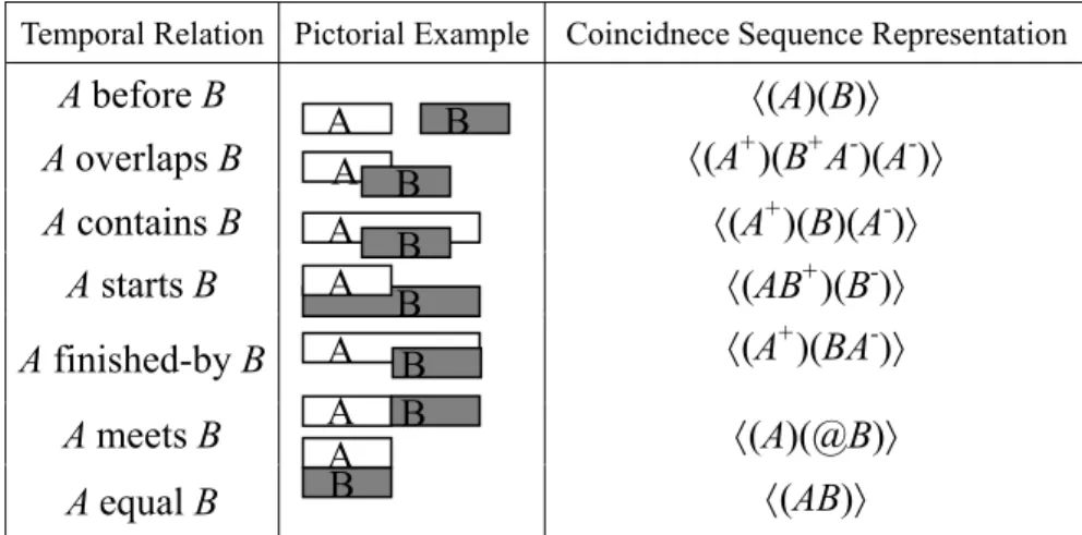
The Allen’s temporal logics between any two events can be mapped to Csequence representation without ambiguity as shown in Table 3-2. To represent temporal relations among more than two events in an event sequence is still unambiguous since it maintains the relative positions of time points of events and additional meet tokens distinguish two adjacent events .

Temporal Relation Pictorial Example Coincidnece Sequence Representation

A before B 〈(A)(B)〉

A overlaps B 〈(A+_)(B+_A-_)(A-_)〉

A contains B 〈(A+_)(B)(A-_)〉

A starts B 〈(AB+_)(B-_)〉

A finished-by B 〈(A+)(BA-)〉

A meets B 〈(A)(@B)〉

A equal B 〈(AB)〉

Table 3-2 Allen’s temporal relations map to coincidence representations.

A A A B A A A B B B B B A B

(31)

The occurrence number is attached to every event of an event sequence to distinguish multiple occurrences of the same event type. In the example shown in Fig. 3-2(a), both event A and B occur twice in the event sequence. After transforming the event sequence to the Csequence, the occurrence numbers are also attached to the corresponding event slices as shown in Fig. 3-2(b). Note that, an event incised to a pair of start slice and finish slice has the same occurrence number. The first occurrence of event A and B incised to a pair of start slice and finish slice with the same occurrence number of 1.

Figure 3-2 Illustration for occurrence numbers in event sequence and its corresponding

Csequence. 2 2 1 1 A B (a) _(b) Csequence: 〈(A1+)(B1+A1-)(B1-)(A2)(B2)〉

(32)

Chapter 4 Projection Scheme

The projection process is a significant contribution of PrefixSpan algorithm, since it partitions both the data and the sets of frequent patterns to be tested, and confines each test to its corresponding smaller projected database. This approach can reduce the search space effectively. For a frequent pattern, we only require searching its corresponding projected database for local frequent items, and then append them to the prefix to form a new frequent pattern.

We extend the projection process of PrefixSpan and do some modification to adapt to coincidence representation. The major concern is to represent each subsequence of an event sequence by coincidence representation correctly. Given an event sequence and its corresponding Csequence, a subsequence of an event Csequence can be treated as choosing some pairs of start slice and its corresponding finish slice and some intact slices to stay in the Csequence and eliminating the rest of event slices. An event is represented as a pair of start slice and finish slice in the Csequence because the event has different extent overlaps with the other k events where k ≥ 1. If the k events are eliminated, the event must be represented as an intact slice instead of a pair of start and finish slices in the Csequence. For example, a sequence of event A obviously is a subsequence of the event sequence “A contains B”. Event A represented in Csequence as 〈(A)〉 is not a subsequence of 〈(A+_)(B)(A-_{)〉, i.e., 〈(A)〉≠} 〈(A+_)(A-_{)〉. Therefore, the merge operation is proposed to transform the Csequence into a new} Csequence which forms a coincidence representation of subsequence of corresponding event sequence correctly. The merge operation is defined as follows.

Definition 7 (merge(α,e+) operation) The merge operation merges the start slice e+ and its

(33)

Csequence α. Then, a new Csequence α’ is generated which is also a subsequence of the Csequence α. Essentially, α’ is a coincidence representation of subsequence of corresponding event sequence with respect to α. The intact slice e is recovered by merging a series of coincidences started with the start slice e+ and finished by the finish slice e- and event slices correlated to the new coincidence need to be adjusted.

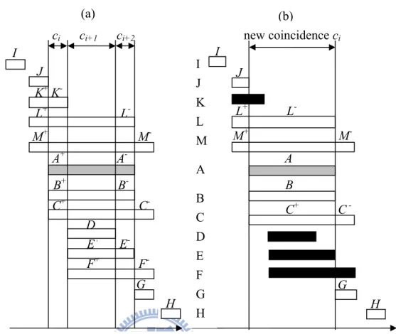
Fig. 4-1 shows all possible events related with event A which is incised to a pair of event slices, i.e., A+ and A-. The event sequence shown in Fig. 4-1(a) contains event A and all its related events B, C, D to M. The coincidence representation of the event sequence is

〈(I)(JK+_L+_M+_)(@A+_B+_C+_K-_)(@DE+_F+_)(A-_B-_E-_L-_)(@GC-_F-_M-_)(H)〉

and we want to merge start slice A+ and finish slice A- to an intact slice A by merging a series of coincidences started with A+ and finished by A-. Three successive coincidences, ci, ci+1 and ci+2, shown in Fig. 4-1(a) are merged to form a new one as shown in Fig. 4-1(b).

Adjustments of 12 events related to event A, i.e., events B, C, D to M, are classified into 3 categories. First, events occur before or after the new coincidence, i.e. events I, J, G and H, do not need any adjustment. Second, events not fully coincident with the new coincidence, i.e. events D, E, F and K, will be omitted. Third, event slices coincident fully with the new coincidence, i.e. events B, C, L and M, remain in the new coincidence. If both start slice and finish slice are of the same event type in the new coincidence ci, we merge the event slices to become an intact slice. After merge operation on event slices A+ and A-, the new Csequence is formed and is represented as 〈(I)(JL+_M+_)(@ABC+_L-_)(@GC-_M-_{)(H)〉 as shown in Fig 4-1(b).}

(34)

Definition 8 (CSubsequence) The subsequence β without single start slice or single finish

slice of Csequence α, i.e., either a pair of start slice and its corresponding finish slice or an intact slice of α appears in the subsequence, is called a Csubsequence of α. Furthermore, the Csequence β’ is generated after multiple merge(e,β) operations where e is a start slice in β, and the β’ is a Csubsequence of α too.

Definition 9 (support count of a Csequence) Given a coincidence database Dc, a tuple 〈sid, s〉 is said to contain a Csequence β, if β is a subsequence of s. The support of a Csequence β

in a coincidence database Dc is the number of tuples in the database containing β, i.e.,

support (β) = | { 〈sid, s〉 | ( 〈sid, s〉 ∈ Dc) ∧ (β s) } |

Given a positive integer min_sup as the support threshold, a Csequence β is called a

coincidence pattern if support (β) ≥ min_sup.

Definition 10 (prefix, projection and postfix)

(b) new coincidence ci ci ci+1 ci+2 I J K L M L+ L -M+ M -I K+ K -J H G F+ F -E+ E -D C+ C -B+ B -A+ A -(a) B C D E F G H A L+ L -M+ M -J I H G C+ C -A B

Figure 4-1 Illustration for merging event slice A+ and A- to form A and adjusting related

(35)

1. prefix: Given a Csequence α = 〈e1,e2,…en〉, a Csequence β= 〈e’1,e’2,…e’m〉 (m ≤ n) is called a prefix of α if and only if (1) β is a Csubsequence of α with least merge operations, that is, there exists a Csequence α’ = 〈e’’1,e’’2,…e’’q〉 (m ≤ q) which is the largest super-sequence of β after least merge operations of α. (2) ei’ = e’’i, for i ≤ m-1 (3) e’m ⊆ e’’m, and (4) all the event slices in (e’’m - e’m) are orderly after those in e’m.

2. projection: Given Csequences α and β such that β is a Csubsequence α and α’ is the largest super-sequence of β with respect to α. A subsequence δ of Csequence α’ (i.e., δ ⊆ α’) is called a projection of α with respect to prefix β if and only if (1) δ has prefix β and (2) there exist no proper super-subsequence δ’ of δ, δ’≠δ, such that δ’ is a subsequence of α’ and also has prefix β.

3. postfix: Let δ= 〈e1e2…en〉 be the projection of α with respect to prefix β= 〈e1e2…em-1e’m〉 (m ≤ n) and α’ is the largest super-sequence of β with respect to α. A CSequence γ = 〈e’’mem+1…en〉 is called the postfix of α with respect to prefix β and α’, denoted as γ=α’/β, where e’’m = (em – e’m). We also denote α’=β．γ. If β is not a subsequence of α’, both projection and postfix of α with respect to β and α’ are empty. An example as shown in Fig. 4-2, 〈(A+_{)〉, 〈(A}+_)(B+_{)〉, 〈(A}+_)(B+_)(C)_{〉, 〈(A}+_)(B+_)(C)(A-_)〉, 〈(A+_)(B+_)(C)(A-_B-_{)〉 are the prefixes of sequence α = 〈(A}+_)(B+_)(C)(A-_B-_{)〉 and 〈(A)〉, 〈(A}+_)(B)〉, 〈(A+_)(B)(A-_{)〉 are also prefixes of α due to merge(α, A}+_{) =α’=}_{〈(A)〉 and merge(α, B}+₎ =α’’= 〈(A+_)(BA-_{)〉. But neither 〈(B}+_{)(C)〉 nor 〈(C)〉 is considered as a prefix of α.} 〈(B+_)(C)(A-_B-_{)〉 is the postfix of the sequence α with respect to prefix 〈(A}+_{)〉, 〈(C)(A}-_B-_{)〉 is} the postfix with respect to prefix 〈(A+_)(B+_{)〉, and 〈(_A}-_{)〉 is the postfix with respect to prefix} 〈(A+_)(B)〉.

(36)

4.1 Multi-projection Technique

In PrefixSpan, the relations between items are only before, after and equal. However, CTMiner not only considers the three relations between event slices but also considers the limitation caused by the characteristic of paired start slice and finish slice. If we adopt projection scheme without considering such limitation, then the obtained information is not sufficient. In other words, the obtained frequent temporal patterns are incomplete. We discuss the limitation and the difference of the projection scheme between PrefixSpan and CTMiner in details as follows.

For example, after projecting the time point-based event sequence S1 = 〈(A1)(B1C1)(A2)(B2D1)〉 with respect to the prefix 〈(A)(B)〉 and the projected sequence 〈(_C1)(A2)(B2D1)〉 will be generated since the pattern (A1before B1) occurs firstly in S. The

(c) (b) (a) c1 c2 c3 c4 A B C (A+) (B+) (C) (A-B-) c1

new coincidence merged by c2 to c4

A B C

(B)

new coincidence merged by c1 to c4 A

B C

(A)

(37)

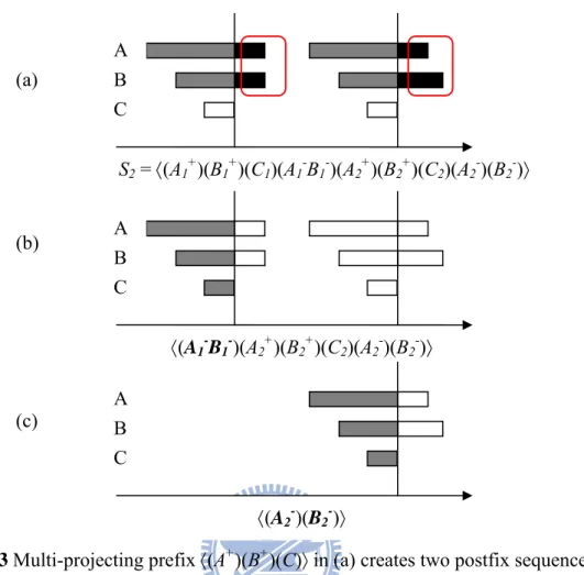
projected sequence is accurate since the relationship between any two time point-based events is simpler. Take another example as shown in Fig. 4-3, the temporal event sequence S2 = 〈(A1+)(B1+)(C1)(A1-B1-)(A2+)(B2+)(C2)(A2-)(B2-)〉 is projected with respect to the prefix 〈(A+_)(B+_{)(C)〉 as shown in Fig. 4-3(a). The pattern A}

1+ before B1+ occurs firstly in S2. If we adopt projection approach of PrefixSpan without considering the limitation, the only projected sequence 〈(A1

-B1-)(A2+)(B2+)(C2)(A2-)(B2-)〉 is generated as shown in Fig. 4-3(b), where A1 -and B1-_{in bold represent the corresponding finish slices of A}

1+ and B1+ in the prefix, respectively. Although the projected result looks fine, actually the obtained information is inadequate. The first occurrence of 〈(A+_)(B+_{)(C)〉 in S}

2 implies the temporal relation between event A and B is (A finished-by B), but the second occurrence of 〈(A+_)(B+_{)(C)〉 implies the} temporal relation is (A overlap B). After the projection, The postfix sequences only keep the first occurrence pattern and ignore the rest of patterns with the same prefix of 〈(A+_)(B+_)(C)〉 since A2- and B2- are not the corresponding finish slices which cannot be appended to the prefix. In other words, for a given pattern, the original projection method forms the projected database from collecting all projected sequences with regards to only the first occurrence of the prefix in each Csequence. In this paper, a new projection strategy called multi-projection is proposed to address this problem.

(38)

Figure 4-3 Multi-projecting prefix 〈(A+)(B+)(C)〉 in (a) creates two postfix sequences (b) and

(c) to obtain complete frequent coincidence patterns.

Multi-projection projects every occurrence of the prefix in Csequences then collects all generated postfix sequences with respect to the prefix with start slices to form the projected database. Therefore, it may generate more than one postfix sequences. From the running example above, multi-projecting a temporal sequence shown in Fig. 4-3(a) with regard to the prefix 〈(A+_)(B+_{)(C)〉 will generate two postfix sequences 〈(A1}

-B1-)(A2+)(B2+)(C2)(A2-)(B2-)〉 and 〈(A2-_)(B2-_{)〉 as shown in Fig. 4-3(b) and Fig. 4-3(c), respectively. Obviously, the size of} projected database constructed by multi-projection is dominated by the proportion of frequent multiple start slice repetitions in the Csequence. With regard to the prefix with start slices, the more occurrences of the prefix in the sequence, the more projected sequences with respect to the prefix will be generated. The workload for multi-projection is additional postfix sequences generation and collection.

S2 = 〈(A1+)(B1+)(C1)(A1-B1-)(A2+)(B2+)(C2)(A2-)(B2-)〉 A B C 〈(A1 -B1-)(A2+)(B2+)(C2)(A2-)(B2-)〉 A B C 〈(A2-_)(B2-_)〉 A B C (a) (b) (c)

(39)

To reduce the memory usage of projected databases caused by multi-projection scheme, we apply the pseudo-projection technique proposed by Pei et al. [5] to address this problem. Instead of performing physical projection, pseudo-projection registers the identifier of the sequence we need to project and the starting position of the projected suffix in the sequence. Then, a physical projection of the sequence is replaced by registering the sequence identifier and the projected position index. With this technique, the usage of memory can be reduced substantially. The projection scheme of CTMiner utilizes pseudo-projection technique to avoid physically copying postfix sequences. Therefore, the running time and memory usage of CTMiner is efficient. The details of pseudo-projection technique are described in [5]. The experimental result shows that the performance of multi-projection in both synthetic data and real data still scales well when processing considerable temporal sequences.

(40)

Chapter 5 Proposed Interval-based Event Mining Algorithm: CTMiner

In this chapter, the new algorithm called CTMiner is proposed to find all frequent temporal patterns. CTMiner utilizes the coincidence-slice concepts to accomplish the frequent time interval-based pattern mining task. It can be decomposed into three phases: incision and

projection, coincidence mining and temporal relation discovery. Chapter 3 describes the

idea and method of incision strategy to transform an event sequence in temporal database into unambiguous Csequences. And we also define prefix, projection and postfix which are different from traditional PrefixSpan algorithm and describe the projection scheme as preliminary of coincidence mining phase. In this Chapter, we will give a high level description of PrefixSpan and details CTMiner algorithm and the proposed three pruning mechanisms for coincidence pattern mining. Finally, we describe the algorithm which transforms frequent coincidence patterns back to temporal patterns in a frequent temporal pattern then discovers all the temporal relations between any two events expressed as a relation list.

In Fig. 5-1, algorithm 1, CTMiner illustrates the main framework. It first scans the temporal database to discover all frequent events and remove infrequent intervals and empty event sequences (Line 2-3, algorithm 1). Then Incision_and_projection is called to transform the original temporal database into coincidence database and get all projected coincidence temporal databases with respect to each frequent 1-pattern (Lines 4, algorithm 1). Then the coincidence mining task CPrefixSpan is called for each projected coincidence database to get frequent coincidence patterns (Lines 5, 6, algorithm 1). Finally, we discover a relation list which illustrates all temporal relations among events in a frequent coincidence pattern by called Temporal_relation_discovery. (Line 7, algorithm 1).

(41)

Algorithm 1: CTMiner ( D,min_sup )

Input: A temporal database D, and the minimum support threshold min_ sup Output: Frequent temporal sequential patterns L

Variables: All frequent coincidence patterns F, all frequent temporal 1-patterns L1, a set P which collects all projected databases with respect each 1-pattern, projected database D |a ∈ P with respect to the prefix a

1: F←∅, L←∅

2: scan temporal database D to find all frequent 1-patterns and remove infrequent intervals and empty event sequences , L1← all frequent 1-patterns.

3: L←L1;

4: P = Incision_and_Projection(L1,D,F, min_sup); //incision phase 5: for each projected database D|a ∈ P do

6: CPrefixSpan(D|a, min_supp, F); //coincidence mining phase 7: Temporal_relation_discovery(F, L); //temporal relation discovery phase 8: output frequent temporal sequential patterns in L;

Figure 5-1 The CTMiner algorithm.

5.1 Phase I: Incision and Projection

Given a temporal database, the events associated with the same SID can be grouped into an event sequence. In incision and projection phase, we scan the temporal database to handle each event sequence. Each event sequence is incised to Csequence then it is projected to the postfix sequences with respect to each frequent 1-event slice as a prefix. The postfix sequences with the same SID are grouped and dispatched to the corresponding projected database. After handling all event sequences, the procedure returns a set of projected coincidence databases with respect to frequent 1-event slices. Algorithm 2 illustrates the details of incision and projection as shown in Fig. 5-2.

First, each event sequence is transformed to Csequence by the following operations (Line1-20, algorithm 2). The information of start/finish time points of each event is added to a list called time_points_list then sorts all the records in the list in the order of time (Line 3,4, algorithm 2). Then the records are grouped into time_list by the same time and Csequence is

(42)

generated simultaneously (Line 5-20, algorithm 2). Two pointers cur_time_list and

last_time_list point to the first two cur_time_lists (Line 7, algorithm 2) and the coincidence is

decided by dealing the records of cur_time_list and last_time_list.

Algorithm 2: Incision_and_Projection(L1,D,F,min_sup)

Input: All frequent temporal 1-patterns L1, a temporal database D, all frequent coincidence patterns F, and the minimum support threshold min_ sup

Output: A set P which collects all projected databases with respect each 1-pattern, Variable: time_list , time_points_list,cur_time_list, last_time_list, coincidence,

sequence, postfix_seq’ ,postfix_seq’’,D|p’, D|p’’

1: for each sequence s in D do 2: sequence←∅;

3: for each interval a in s do

4: add the information of time points of a (a.time,a.event_type,a.type) to

time_points_list.

5: sort records in time_points_list by time and event type in increasing order; 6: grouping the records in time_points_list with the same time into time_list; 7: cur_time_list and last_time_list point to the first two time_list;

8: while cur_time_list is not points to a null time_list do, 9: coincidence←∅;

10: if there exist two records i, j with type start and finish respectively in

last_time_list do

11: coincidence← coincidence ∪ “@”; //meet token 12: for each record r in last_time_list do

13: if r.type = start then //start slice 14: coincidence← coincidence ∪ “r.event_type” with “+”; 15: for each record r in time_list do

16: if r.type = finish then //finish slice 17: coincidence← coincidence ∪ “r.event_type” with “-”; 18: merge start slice and finish slice with same event type to an intact

slice in coincidence; //intact slice 19: sequence ← sequence ◇ 〈 coincidence 〉;

20: last_time_list and cur_time_list point to next time_list; 21: for each frequent 1-pattern p in L1 do

22: create start slice p’ and intact slice p’’ of p.

(43)

24: postfix_seq1 = projection_to_coincidence_seq(sequence,p’’); 25: D|p’ ← D|p’ ∪ postfix_seqes ;

26: D|p’’ ← D|p’’ ∪ postfix_seq1 ;

27: for each projected coincidence database D|prefix do, 28: If |D|prefix| ≥ min_supp then

29: P ← P ∪ D|prefix ; 30: output P;

Figure 5-2 The Incision_and_Projection algorithm.

If two records with different types exist in last_time_list then the meet token “@” is placed into coincidence to distinguish from two adjacent events (Line 10, 11, algorithm 2). Note that, the type indicates the time point either a stp or a ftp. The start slices with corresponding stps in last_time_list are created and placed into the coincidence and the finish slices with corresponding ftps in cur_time_list are also created and placed into the coincidence (Line 12-17, algorithm 2). If the start slice and the finish slice in the coincidence have the same event type, we combine them to form an intact slice (Line 18, algorithm 2). Then the ordered coincidence formed a Csequence (Line 19, algorithm 2). For each frequent 1-pattern p, two projected coincidence databases with respect to a start slice and an intact slice of p are generated to handle the temporal patterns beginning with the start slice and the intact slice, respectively (Line 21-26, algorithm 2). Output all projected coincidence databases with the number of Csequences greater than the minimal support (Line 27-30, algorithm 2). Finally, the temporal database has transformed to a set of projected coincidence databases which consist of start slices, finish slices, intact slices and meet toke. For the example as shown in Fig. 5-3, Incision_and_Projection operates on event sequence 3 in Table 3-1. The

cur_time_list is pointing to the 6th time_list and the last_time_list always points to the

previous time_list which cur_time_list is pointing to, i.e., the 6th time list = {E+}. First, we check if there exist both start slice and finish slice in last_time_list to distinguish two adjacent events then put all start slices in last_time_list and all finish slices in cur_time_list into coincidence, i.e., (E+E-). The same event with both start slice and finish slice in coincidence