A Particle-Swarm-Driven Cross-Entropy Method
for Multiple-Input-Multiple-Output Signal
A Particle-Swarm-Driven Cross-Entropy Method for
Multiple-Input-Multiple-Output Signal Detection
Student : Chun-Lin Wang
Advisor : Dr. Yu T. Su
A Thesis
Submitted to Department of Communications Engineering
College of Electrical and Computer Engineering
National Chiao Tung University
in partial Fulfillment of the Requirements
for the Degree of Master of Science
in Communications Engineering
August 2009
(MIMO)
(zero-forcing)
(minimum-mean-square-
error)
(sphere decoding)
(V-BLAST)
(lattice reduction)
(maximum likelihood)
(cross-entropy)
(Monte-Carlo)
Kullback-Leibler
(importance
sampling density)
(BER)
(SNR)
(error floor)
(particle swarm algorithm)
A Particle-Swarm-Driven Cross-Entropy Method for
Multiple-Input-Multiple-Output Signal Detection
Student : Chun-Lin Wang Advisor : Yu T. Su
Department of Communications Engineering National Chiao Tung University
Abstract
Many solutions for detecting signals transmitted over flat-faded multiple input multi-ple output (MIMO) channels have been proposed, e.g., the zero-forcing (ZF), minimum mean squared error (MMSE), lattice reduction and V-BLAST algorithms, to name a few. However, these approaches suffer from either unsatisfactory performance or high complexity.
We present an alternative method for detecting quadrature amplitude modulated (QAM) MIMO signals. This method tries to estimate the probability distribution of the candidate signal location by sampling over a neighborhood of the received wave-form. The proposed random sampling based iterative distribution estimator is similar to the class of Monte-Carlo based optimization approach and if the distance used in measuring the distance between a tentative distribution and the optimal distribution is the Kullback-Leibler distance (cross entropy) then our solution is identical to the one known as the Cross-Entropy (CE) method. The CE method is motivated by the search for an efficient rare-event simulation solution. The problem is equivalent to finding the optimal importance sampling density. The desired density is obtained by iterative random search in the space of exponential distributions with the CE metric.
The proposed CE-based detector yields bit-error-rate (BER) performance which is close to that achievable by the Maximum-Likelihood (ML) detector when the signal-to-noise ratio (SNR) is relatively low. Unfortunately the performance curves exhibit error floors in high SNR region. To improve the performance in high SNR region, we borrow the concept of particle swarm optimization (PSO) in designing our detector. PSO is a population-based iterative search algorithm which moves a number of particles through the feasible solution space towards the optimal solution with the information obtained in previous iterations. The modified iterative detector incorporates extra terms, which are generated by a PS-like process and represent a driving force to pull the iterative op-timization process from being trapped in local minimums, in updating of the importance density and is called the particle-swarm-driven cross-entropy (PSD-CE) MIMO detector. The PSD-CE detector gives significant BER performance improvement in medium-to-high SNR region. We also consider the case when channel state information is imperfect and suggest a robust detector structure based on a modified score function.
Contents
Chinese Abstract i
English Abstract ii
Acknowledgement iv
Contents v
List of Tables vii
List of Figures viii
1 Introduction 1
2 System Model 5
2.1 Perfect Channel Estimation . . . 5
2.2 Pilot-based Channel Estimation . . . 7
3 General MIMO Detection Schemes 9 3.1 Linear Detectors . . . 9
3.1.1 Zero Forcing Dector . . . 9
3.1.2 Minimum Mean Squared Error Detector . . . 10
3.2 Nonlinear Detectors . . . 10
3.2.1 Maximum Likelihood Detector . . . 10
4 Particle Swarm Optimization 13
4.1 Particle Swarm Algorithm . . . 13
4.2 Variations of Particle Swarm Algorithm . . . 17
5 Cross-Entropy-based MIMO Signal Detection 19 5.1 Generic Cross-Entropy Method . . . 19
5.1.1 Importance Sampling . . . 19
5.1.2 A Generalized CE Method for Optimization . . . 20
5.2 Cross-Entropy-based MIMO Signal Detection . . . 21
5.2.1 A CE-based MIMO detection algorithm . . . 21
5.2.2 Weighting Factors . . . 23
5.2.3 Simulation Result of the CE-based Detection Method . . . 24
5.3 Particle-Swarm-Driven Cross-Entropy Methods . . . 24
5.3.1 A PS-Driven CE MIMO Detection Algorithm . . . 24
5.3.2 Modifications for the PS-Driven CE Method . . . 28
5.4 Score Function under Imperfect Channel Estimation . . . 29
6 Simulation Results 31 6.1 Perfect Channel Estimation . . . 31
6.2 Imperfect Channel Estimation . . . 37
6.3 Complexity Comparison . . . 38
7 Conclusion 40
List of Tables
3.1 The V-BLAST detection algorithm. . . 12
5.1 The cross-entropy-based MIMO detection algorithm. . . 23
5.2 The Particle-Swarm-driven CE MIMO detection algorithm. . . 28
List of Figures
2.1 A MIMO system model. . . 6 4.1 Vector representation for relationship between velocity and position with
k = 2. . . . 15 4.2 The Particle Swarm algorithm flow chart. . . 16 4.3 Two examples for neighborhood topology. . . 18 5.1 BER performance comparison of ML detection and the CE-based
detec-tion with α = 0.3. . . . 25 5.2 An example of region of A0
M as a = 1 + i with 16-QAM. . . . 27
6.1 BER performance of the two proposed detectors. . . 32 6.2 BER performance comparison of different detectors. . . 32 6.3 BER comparison of the PS-driven CE detector using(1) xg(1) only; (2)
both xg(1) and xp(1). . . 33
6.4 BER comparison of the PS-driven CE detector using xg(1) and (1) xp(1);
(2) xp(2); (3) xp(3), respectively. . . 34
6.5 BER comparison of the PS-driven CE detector using xg(1) and xp(2) with
different weighting of xp(2). . . 35
6.6 BER comparison of the PS-driven CE detector using (1)xg(1) and xp(2);
(2)xg(1), xg(2) and xp(2). . . 35
6.7 Symbol error rate performance of the PS-driven CE detector using xg(1)
6.8 The averaged minimum distance at each iteration when SNR=15 dB. . . 36 6.9 BER of a 6 × 6 MIMO system with 4-QAM under the PS-driven CE
detection algorithm and ML detection. . . 37 6.10 BER performance comparison of a 4×4 MIMO system with 4-QAM based
on different score functions with σ2
Chapter 1
Introduction
Wireless communications are impaired predominantly by multipath fading [2]. How-ever, in a richly scattered fading environment, fading can be beneficially as it promises a multiple-input-multiple-output (MIMO) system to achieve significant capacity gain through independent spatial modes [1]. For this reason, the MIMO technology has gained enormous popularity and attracted much research interest over the past decade [2]. Depending on the operation environment, a MIMO system possesses the potential to obtain (1) array gain, (2) spatial diversity gain, (3) spatial multiplexing gain and (4) interference reduction capability [1, 2].
Array gain refers to the increase in receive SNR through spatial processing at the
receive antenna array and/or spatial pre-processing at the transmit antenna array. It improves the coverage and the range of a wireless network by raising resistance to noise.
Spatial diversity gain alleviates fading of the signal level by providing the receiver with
multiple copies of the transmitted signal in space, frequency or time. Ideally, these copies are independent and the number of independent copies is called the diversity order. The quality and reliability of the received signal improves as diversity order increases. A MIMO channel with NT transmit antennas and NR receive antennas offers a spatial
diversity order of NTNR. Transmitting multiple and independent data streams within
the operating bandwidth increases data rates and capacity of a wireless network, which is known as Spatial multiplexing gain [2]. In general, the number of data streams that
can be provided by a MIMO channel equals the minimum of the number of transmit antennas and the number of receive antennas, i.e. min{NT, NR}. Exploiting the spatial
dimension in a MIMO system might alleviate interference caused by sharing resources. In addition, directing signal energy towards the intended user rather than other users would avoid the impact of the interference. Interference reduction and avoidance improve the coverage and range of a wireless network [2].
Although these advantages can not exist simultaneously due to conflicting demands on the spatial degrees of freedom, some combinations across a wireless network would improve the system performance such as capacity and reliability.
Encouraged by the collective behavior of social animals such as fish schooling and the colony of ants, many genetic algorithms have been studied. In the work of Kennedy and Eberhart [3], Particle Swarm Optimization is motivated by bird-flocking behavior and is an iterative algorithm based on social-psychological model of social influence and social learning [4]. In the original model, individuals in a particle swarm follow a simple behavior. The collective behavior that emerges is that of discovering optimal regions of a high dimensional search space. At each iteration, each individual determines its nearest neighbor and replaces its velocity with that of its neighbor. To further extend the model, the “rooster” concept of Heppner and Grenander [5] was added, in the form of a memory of previous best and neighborhood best positions. The previous (personal) best position of each individuals is the best position found by the individual since the first simulation to the current iteration. The neighborhood best position is the best position found by the neighborhood. These two best positions serve as the attractor and the resulting model was referred to as particle swarm optimization. The swarm algorithm exhibits adaptive behavior since the state changes when personal best and global best position change.
The Cross-Entropy (CE) method is a general Monte Carlo approach to solve com-binatorial and continuous multi-extremal optimization problems. The name is derived
from the cross-entropy distance (or the Kullback-Leibler distance) [6] which defines a distance between two probability density functions. This method was animated by an adaptive algorithm including the idea of minimizing variance for estimating probabilities of rare events in complex stochastic networks [7]. Soon after the first exploration, the fact was found that a simply modified version could be used not only for estimating probabilities of rare events but for solving difficult combinatorial optimization problems as well. This is done by translating an original deterministic optimization problem into a related stochastic estimation problem and applying the rare-event simulation mechanism to it [8].
The CE method is an iterative procedure and each iteration involves two phases [9] : 1. Generate a set of random samples according to a specified mechanism.
2. Update the parameters of the random mechanism based on the generated data in order to produce a better set of samples in the next iteration.
The advantage of the CE method is that it provides a simple adaptive procedure for estimating the optimal reference parameters. The fact that the updating rules are simple, explicit and optimal in some well-defined mathematical sense makes the CE method powerful and desirable. It provides a unifying approach to simulate and optimization and has great potential for exploring new search areas in the solution space.
The rest of this thesis is organized as follows. The ensuing chapter provides brief summary of the assumptions and models for the channel and system of concern. In Chapter 3, we review some general MIMO detection schemes including linear and non-linear detection methods. Chapter gives a detailed description of the Particle Swarm Algorithm. In the following chapter, the concepts of the cross-entropy-based MIMO detection method as well as the particle-swarm-driven cross-entropy MIMO detection method are proposed. Chapter 6 shows simulation performance of these algorithms are provided. Finally, our work is concluded. The notations used in this thesis are as follows.
Vectors and matrices are denoted by symbols in bold face. (·)T and (·)H represent
trans-pose and Hermitian transtrans-pose, respectively. E{·} denotes the statistical expectation. tr(·) denotes the trace of an square matrix.
Chapter 2
System Model
2.1
Perfect Channel Estimation
Consider a MIMO system with NT transmit antennas and NR receive antennas
with NR > NT. Input data is demultiplexed into NT substreams which are mapped
onto sequences of M-QAM symbols. The set of candidate signals in the constellation is denoted as AM. These substreams are transmitted simultaneously and received
syn-chronously. For convenience but without loss of generality, we present a time-discrete complex baseband model for one time slot only.
Let xi and yj denote the complex valued signal transmitted by the ith antenna and
those received by the jth receive antenna, i = 1, · · · , NT, j = 1, · · · , NR, respectively.
Denote H as the overall channel matrix and assume, for the time being, that H is perfect known to the receiver. In other words, there is no channel estimation error at the receiver. The (j, i)th element of H, hj,i, is the channel response between the ith
transmit antenna and the jth receive antenna. The MIMO system model just described is shown in Fig. 2.1. The received signal (vector) expressed in matrix form is given by
Figure 2.1: A MIMO system model. where x = [x1, · · · , xNT] T ∈ ANT M , (2.2) y = [y1, · · · , yNR] T ∈ CNR, (2.3) w = [w1, · · · , wNR] T ∈ CNR, (2.4) H = h1,1 · · · h1,NT ... . .. ... hNR,1 · · · hNR,NT ∈ CNR×NR. (2.5)
and C denotes the complex-valued domain. Every element of H is a complex Gaussian fading gain with unit variance, i.e. σ2
h = 1. The vector w represents the complex
additive white Gaussian noise with zero mean and variance σ2
w. Each noise observed at
the different antenna is assumed to be uncorrelated, i.e. E{wwH} = Σ
w = σw2INR where INR is an identity matrix of size NR× NR. Throughout our work, the average transmit power of each antenna is also normalized to 1. In other words, x has a covariance matrix E{xxH} = σ2
xINT with σ
2 x = 1.
2.2
Pilot-based Channel Estimation
In practice, the assumption that H is perfect known by the receiver is not valid. There usually exists differences between the exact channel matrix and the estimated channel matrix due to channel estimation errors.
In order to estimate the channel matrix H by the receiver, a number of pilot symbols are sent prior to data symbols. Denote by si the NP × 1 pilot vector for ith transmit
antenna and constitute the NT × NP matrix S as
S = sT 1 ... sT NT . (2.6)
The receive vector yP follows to
yP = HS + wP (2.7)
where wP is AWGN noise with zero mean and covariance matrix σw2PINR.
Define the channel matrix estimation error as ∆H, the channel known at the receiver can be written as
ˆ
H = H + ∆H, (2.8)
and the linear least-square (LS) estimate of H is given by ˆ
H = yPSH(SSH)−1. (2.9)
We thus have
∆H = wPSH(SSH)−1 (2.10)
It is known that mutual orthogonal pilot sequences will obtain the best channel estimate with uncorrelated estimation errors. Therefore, the rows of S are chosen to be orthogonal, i.e.
SSH = N
where EP is the average power of the training symbols defined as
EP =
1
NPNT
tr(SSH). (2.12)
From [10], the conditional probability density function (PDF) of ˆH given H is a complex Gaussian distribution with mean H and covariance matrix Σ∆H = σ2∆HINT. Using the PDFs of H and ( ˆH|H) with the conditions of mutually orthogonal pilot sequences and i.i.d. channel coefficients, we derive the PDF of (H| ˆH) as [10]
p(H| ˆH) = CN (δ ˆH, δσ2 ∆HINT ⊗ INR) (2.13) with δ = σ 2 h σ2 h+ σ2∆H (2.14) where CN (·) denotes complex Gaussian distribution and ⊗ represents the Kronecker product.
Chapter 3
General MIMO Detection Schemes
We briefly survey four classes of popular MIMO detection schemes in this chapter for the convenience of subsequent discussions. These detectors are classified into two categories, namely, the linear and nonlinear detection schemes.
3.1
Linear Detectors
Using a NT × NR matrix P to linearly combine the elements of the received signal
y is a straightforward approach to estimate the transmit signal x. Zero-Forcing (ZF) and Minimum-Mean-Square-Error (MMSE) are the most two common methods in linear MIMO detection schemes.
3.1.1
Zero Forcing Dector
In a ZF detector, the interference introduced by the channel matrix is nulled out by multiplying the received signal vector y with the Moore-Penrose pseudo-inverse [11] of the channel matrix, i.e. PZF = H+ = (HHH)−1HH. The transmit signal x is estimated
by quantizing every element of the filter output vector to an element of the symbol alphabet,
ˆ
x = Q{H+y} = Q{x + (HHH)−1HHw}, (3.1)
A drawback of a ZF detector is that nulling out interference without considering the noise might amplify the noise power significantly. For an orthogonal channel matrix, ZF is identical to the optimum detector, Maximum Likelihood (ML) detector. However, since the channel matrix is not ideal or orthogonal in practice, ZF leads to a noise enhancement problem generally.
3.1.2
Minimum Mean Squared Error Detector
To solve the noise enhancement problem in ZF detectors, MMSE detectors take the noise term into account and minimize the mean square error between the transmit signal and the estimated transmit signal, J(P) = E{(x − ˆx)H(x − ˆx)}, with respect to P. The
optimum matrix PM M SE is given by
PM M SE = µ HHH + σ 2 w σ2 x ¶−1 HH. (3.2)
Similar to ZF detectors, each element of the filter output is mapped by a minimum distance quantization so as to get the estimated transmit signal.
3.2
Nonlinear Detectors
3.2.1
Maximum Likelihood Detector
The maximum likelihood (ML) detector estimates the transmit signal ˆx by find-ing the one which minimizes the distance between the received signal vector and the estimated signal vector, i.e.
ˆ
x = arg min
x∈ANTM
||y − Hx||. (3.3)
The problem can be solved by exhaustively searching over all possible x and choose the one that makes the distance smallest. However, although ML has the best performance among all MIMO detection algorithms, the number of all possible x increases with
NT exponentially. The computational complexity will become prohibitively high when
transmit antenna NT and constellation size M increase.
3.2.2
V-BLAST Algorithm
Vertical Bell Labs layered space time algorithm (V-BLAST) is a popular nonlinear combining approach for detecting MIMO signals [12]. V-BLAST detection employs an ordered serial detect-and-cancel strategy similar to that of decision-feedback equalizer. At the receiver, a successive interference cancellation concept is applied such that each substream is considered as the desired signal in turn while the others are regarded as interferers. With a linear combinatorial nulling technique, nulling is performed in a particular detection order by linear weighting the received signals to satisfy a specific criterion such as ZF or MMSE. Taking ZF nulling for example, the weighting vectors zi
of size NR× 1 for i = 1, · · · , NT are chosen to meet
zT
i (H)j = δij. (3.4)
where (H)j is the jth column of H and δ is the Kronecker delta. And the ith substream
is estimated by
ˆ
xi = Q(zTi y). (3.5)
Interference from already-detected components of x is subtracted out from the received signal. Therefore, the received vector is modified iteratively and the interferers are less than that at the previous iteration. Due to the symbol cancellation used in this algorithm, the weighting vectors for ZF nulling can be revised as
zT
i (H)j =
½
0, if j ≥ i
1, if j = i (3.6)
Denote the detection order set by O = {s1, · · · , sNT}. The general detection process is described in Table 3.1.
Step 1 : Set k = 1.
Step 2 : Choose the nulling vector zsk for skth substream in accordance with equation (3.6).
Step 3 : Calculate the decision statistic for skth substream and quantize it
to obtain ˆxsk as equation (3.5)
Step 4 : Assume ˆxsk = xsk, and suppress the component of xsk from the received signal y. Modify the received vector as y = y − ˆxsk(H)j.
Step 5 : Stop at iteration k = NT; otherwise, let k = k + 1 and go back to Step 2.
Table 3.1: The V-BLAST detection algorithm.
The detection order plays an important role in this algorithm. An improper order will induce a error propagation problem. It is proved in [12] that the optimal detection order is determined to maximize the minimum post-detection signal-to-noise ratio (SNR) of all data streams. Therefore, selecting the “best” (smallest) post-detection SNR at each stage in the process leads to the global optimum ordering. The post-detection SNR for detected component xsk of x is obtained by
ρsk = E{|xsk| 2} σ2 w||zsk||2 (3.7) where the expectation is taken over the constellation set.
Chapter 4
Particle Swarm Optimization
4.1
Particle Swarm Algorithm
Inspired by the movements of birds flocking, the particle swarm algorithm is an optimization technique for a real-valued multidimensional solution space [4, 14]. It ad-justs the trajectories of a population of “particles” (or samples) through the feasible solution space iteratively. Every particle is evolved based on the information about each particle’s previous best performance and the best previous best performance of its neighborhood. They traverse a solution space where a quality measure, fitness can be evaluated. Through cooperation and competition among these particles over several it-erations, all particles can move towards the optimal position. This approach is attractive due to its advantages of the simple mathematical model, resistance to being trapped in a local optimum and faster convergence. For MIMO detection, binary particle swarm optimization (PSO) are applied.
The coordinates of every particle represent a possible solution associated with two vectors, the position and the velocity. In binary PSO, the elements in velocity vector is squashed by a sigmoid function, Sig(x) = 1
1+e−x, to the range (0, 1) and is used to determine whether the corresponding elements in position vector is either 0 or 1. In K-dimensional search space, the ith particle is represented by the position vector
xi = [xi1, · · · , xiK]T and the velocity vector vi = [vi1, · · · , viK]T. In a MIMO detection
problem, xi is regarded as a candidate solution. Applying the PS algorithm to this
problem, the fitness function is defined as
f (x) = ||y − Hx||2. (4.1)
A fitness value of a particle is assigned to the particle’s current location by using the coordinates of the particle. Also, let gb and pb
i denote the position vector of the particle
with the best performance among its neighbors so far and the position vector of ith particle with the best performance along its previous fitness values, respectively.
Velocity vector vi at tth iteration is updated according to the following equation:
vik(t) = vik(t − 1) + φ1[pbik− xik(t − 1)] + φ2[gkb − xik(t − 1)]
with vik ∈ {−vmax, vmax} (4.2)
for k = 1, · · · , K, where φ1 and φ2 are positive random numbers drawn from a uniform
distribution with a predefined upper limit. In binary PSO, the limit is arbitrary but the sum of φ1 and φ2 are usually set to be less than 4 [14]. The first term in equation
(4.2) indicate the impact of the velocity at (t − 1)th iteration. The last two terms are considered as cognitive part and social part, respectively. The cognitive part denotes the effect of the evolution of ith particle itself. The social part represents the interaction between ith particle and its neighborhood.
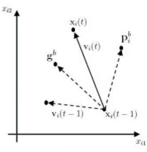
In continuous PSO, the position vector is updated by the velocity vector as [15] xi(t) = xi(t − 1) + vi(t − 1). (4.3)
where t is the index of iteration. Vector representation for relationship between velocity and position is shown in Figure 4.1. In binary PSO [15], the elements in velocity vector after being squashed represents the probabilities of the elements in position vector taking the value 1. To update the position vector xi at tth iteration, the binary decision rule
Figure 4.1: Vector representation for relationship between velocity and position with
k = 2.
shown below is followed:
If rand() < Sig(vik(t)), then xik(t) = 1
else, xik(t) = 0 (4.4)
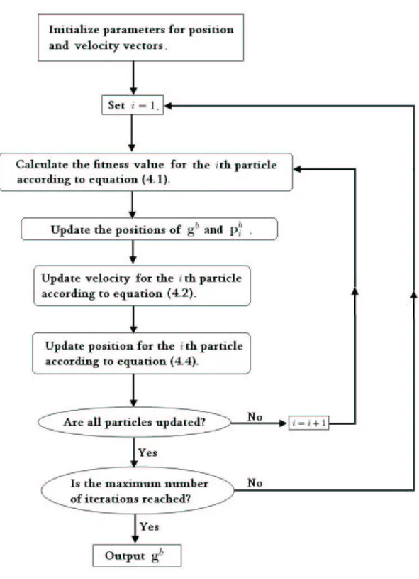
for k = 1, · · · , K, where rand(·) is a random number selection function from a uniform distribution in [0, 1]. With these new position vectors, fitness values of the particles are evaluated. In the meanwhile, gb and pb
i are updated again, and so on. This procedure
is repeated until maximum number of iterations is reached and the estimated transmit signal is decided by gb. The flow diagram of the Particle Swarm algorithm is shown in
4.2
Variations of Particle Swarm Algorithm
In the PS algorithm, there are some parameters related to convergence speed and performance, such as the number of particles in the swarm, the neighborhood topology and the acceleration coefficients [4, 14]. The influences of these basic parameters are discussed in this section.
The more number of particles in the swarm, also called the swarm size, the larger the initial diversity of the swarm. A wider range of search space will be explored at each iteration if the swarm size is larger. Furthermore, it is more possible that more particles would reach the optimal solution within fewer iterations. Nevertheless, the computational complexity increase while a large swarm size is used and the swarm degrades to a parallel random search. Generally, fewer particles are needed for a smooth search space than that for a rough surface. The optimal swarm size is problem-dependent and is suggested to be optimized for each problem through cross-validation methods instead the heuristics found in publications.
In the PS algorithm, gb denote the position vector of the particle with the best
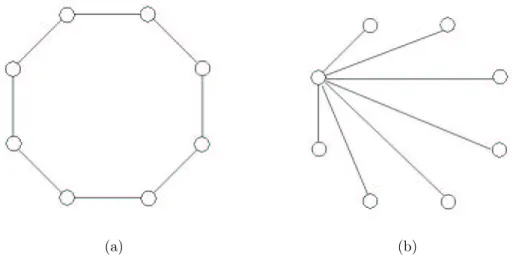
performance among its neighbors. The neighborhood size represents the quantity of social interaction occurring within the swarm. Smaller neighborhood sizes leads to a slow convergence and are insensitive to a local minimum, thus there are more dependable convergence to the optimal solution. To ensure an initial high diversity with faster convergence, the search can start with small neighborhoods. As the number of iterations increases, the size of neighborhood should be enlarged so as to move all particles to a promising search area. Two extreme cases for neighborhood topology are presented in Figure. 4.3. In Figure. 4.3(a) the neighborhood of every particle are the ones next to it while the neighbors for every particle in Figure. 4.3(b) are all other particles in the swarm .
In equation (4.2), the two random numbers φ1 and φ2 are regarded as acceleration
(a) (b)
Figure 4.3: Two examples for neighborhood topology. over the procedure.
Particles move through smooth trajectories if φ1 and φ2 are small. They might
explore more good areas rather than being stocked in a good region found before. On the contrary, large values for φ1 and φ2 lead to more acceleration, and particles move
towards past good regions with hasty movements.
Initialization for φ1and φ2 are important because an improper initialization may lead
to divergent or cyclic behavior over the algorithm. In general, φ1 and φ2 are optimized
Chapter 5
Cross-Entropy-based MIMO Signal
Detection
5.1
Generic Cross-Entropy Method
5.1.1
Importance Sampling
The Cross Entropy (CE) method attempts to solve an optimization problem by relating it to a rare event simulation problem [9]. Usually, the sample size for estimat-ing a rare event probability is very large. Important Samplestimat-ing (IS) is a well-known technique used to reduce the variance by simulating a system under a different set of parameters (reference parameters) or under a different probability distribution. With this technique, the rare event is much more likely to occur so that the sample size of the rare event simulation can be reduced. In conventional IS, the optimal reference parameters are difficult to obtain. The CE method provides a simple and fast proce-dure to estimate the optimal reference parameters used in IS. More specifically, the CE method is an iterative Monte-Carlo based approach to find the IS density, i.e. the im-portance distribution, which is closest to the optimal important distribution in the Kullback-Leibler sense. The Kullback-Leibler distance D(g, h) is a distance measure of
two different distributions g(x) and h(x) which defines as follows:
D(g, h) =
Z
g(x) lng(x)
h(x)µ(dx). (5.1)
A distance metric must satisfy the three rules below: (1) The distance is non-negative.
(2) Symmetric property: The distance between two points is the same while measuring from either direction.
(3) Triangle inequality: Considering a triangle formed by three points, the sum of any two edges is larger than the third edge.
Therefore, the K-L distance is not a true distance metric since it is not symmetric and does not satisfy the triangle inequality.
5.1.2
A Generalized CE Method for Optimization
In this subsection, we give a brief description to the relationship between IS and the CE method for optimization problem. The CE method attempts to solve the following optimization function
arg max
ω∈Ω S(ω) (5.2)
where Ω is the domain of variable ω and S is the score function of ω defined on Ω. Applying IS to this problem, we find another set of parameter, e.g. v, instead of ω. To find the optimal importance distribution within a class of densities f (ω; v), we adapts the parameter v iteratively so that the Kullback-Leibler distance (i.e. the cross entropy) between the associated density and the optimal importance distribution is minimized. In general, a generic CE method can be described by the following steps :
1. Generate samples according to the importance distribution determined at the pre-vious iteration.
2. Calculate the scores to the generated samples according to a specific score function. 3. Update the importance distribution by the samples with comparatively better
scores.
4. Repeat the above steps until the stopping criterion is reached.
At the very beginning, we give a initial distribution to the importance distribution and generate a set of samples depending on it. Then we compute the scores for every sample individually. For an optimization problem, the value of the objective function are usually regarded as the score for each sample. The samples with better scores are called elite samples and the set composed of elite samples is defined as the elite set. We choose those elite samples to update the importance distribution. The updated importance distribution is a linear combination of the original importance distribution and the distribution determined by the elite samples. Again, new samples are generated according to the updated importance distribution and the same steps mentioned above are repeated. This procedure is processed iteratively until the stopping criterion is reached.
5.2
Cross-Entropy-based MIMO Signal Detection
5.2.1
A CE-based MIMO detection algorithm
To apply the CE method to a MIMO system, we first define a score function
S(x) = ||y − Hx||2 (5.3)
under the assumption of perfect channel estimation for solving the following optimization problem,
arg min
x∈ANTM
Following the procedures of the CE method, the importance distribution of x with relatively smaller scores are estimated by minimizing the distance between the initial distribution and the optimal importance distribution. The estimated transmit signal ˆx is the symbol that is the most likely to occur according to the distribution or the sample with the smallest score during the whole process. Intuitively, an estimated transmit signal vector ˆx is regarded as a sample and the score will be calculated for the sample. However, there are MNT possible candidates if we treat a vector as a sample unit. Thus a large sample size may be required to cover a wider search region so that the computing complexity would inevitably increase. In order to avoid this problem, the importance distribution of every element in a transmit signal x is estimated separatively.
Let f(k)(x
i) denote the importance distribution of the ith element for i = 1, · · · , NT,
where the superscript k is the index of iteration. U samples, xk
i,u for u = 1, · · · , U ,
are generated at kth iteration in accordance with f(k)(x
i) for the ith element. To
cal-culate the scores for these samples, a vector set {xk
u}Uu=1 is constructed where xku =
[xk
1,u, · · · , xki,u, · · · , xkNT,u]
T represents the uth sample vector at kth iteration.
Given a specific quantile probability ρ, there are infinite number of thresholds such that the probability of the scores less or equal to these thresholds are larger or equal to
ρ. To select elite samples, we choose the threshold at kth iteration γk satisfying
γk= arg min
γ P (S(Z) ≤ γ) ≥ ρ for Z ∈ {x k
u}Uu=1 (5.5)
And the elite samples are those whose scores satisfies S(xk
u) ≤ γk. The distributions of
elite samples are calculated as
f(k) s (xi = a) = PU u=1I{S(xk u)≤γk}I{xki,u=a} PU u=1I{S(xk u)≤γk} (5.6) where a ∈ AM for i = 1, · · · , NT.
Based on these elite samples, the importance distributions f(k)(x
i) for i = 1, · · · , NT
are updated according to
where α is the weighting factor and 0 ≤ α < 1. The updated importance distributions are linear combinations of the original importance distributions and the distribution of the elite samples.
The procedure described above is repeated iteratively until the stopping criterion is met. For example, the pre-defined number of iterations is reached or the importance distributions converges. This algorithm is listed as shown in Table 5.1.
Step 1 : Initialize the importance distributions f(k)(x
i) with uniform
distribution for i = 1, · · · , NT, respectively. And set k = 0.
Step 2 : Generate U samples xk
i,u from fk(xi) for u = 1, · · · , U.
Construct the set {xk
u}Uu=1 where xku = [x1,uk , · · · , xki,u, · · · , xkNT,u]
T.
Step 3 : Calculate the set of scores {S(xk
u)}Uu=1 according to equation (5.3).
Step 4 : Set a quantile parameter ρ such that there is a γk satisfying
equation (5.5).
Step 5 : Calculate the distribution of elite samples in accordance with equation (5.6).
Step 6 : Update the importance distributions according to equation (5.7). Step 7 : Stop at iteration k = K if the pre-defined stopping criterion is
met; otherwise, let k = k + 1 and go back to Step 2.
Table 5.1: The cross-entropy-based MIMO detection algorithm.
5.2.2
Weighting Factors
In equation (3.6), the weighting factor α effects the exploration and exploitation ability. Exploration is an ability to explore more different regions in the search space to find the global optimum. On the contrary, exploitation is an ability to concentrate the search around the a specific region in order to refine a candidate solution. If α is
larger, the component of updated distribution depends on more information from elite samples. Therefore, it is more likely to exploit than to explore and the convergence speed is faster. However, it is also much more possible to trap in one area since the elite samples generated at first several iterations may lead to a local minimum. If α is small, it takes more iterations to converge but has a higher probability to locate the global optimum.
Usually, to balance the exploration and exploitation, the weighting of the original importance distribution, i.e. the importance distribution at the previous iteration, is about twice that of the distribution of elite samples from some experiences of simulations. Therefore, α is chosen to be about 0.3 in our work. For other optimization problems, it depends.
5.2.3
Simulation Result of the CE-based Detection Method
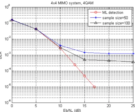
Figure 5.1 shows the BER performance of ML detection and the CE-based detection method under a 4 × 4 MIMO system using 4-QAM.
As shown in the figure, our simulation indicates that the resulting BER performance is close to that of ML detector at low SNR region. However, there exists an error floor when SNR is larger than about 10dB since the estimated importance distributions do not converge uniformly, i.e., some of the importance distributions do converge but not all the NT importance distributions.
5.3
Particle-Swarm-Driven Cross-Entropy Methods
5.3.1
A PS-Driven CE MIMO Detection Algorithm
Inspired by the evolution concept of swarm algorithm, the updating formula of im-portance distribution, i.e. equation (5.7), in the CE-based MIMO detection method
Figure 5.1: BER performance comparison of ML detection and the CE-based detection with α = 0.3.
is modified to solve the problem of nonuniform convergence mentioned in the previous section. The main idea is to keep the newly generated samples close to the generated samples with the best scores. Except for the elite samples generated in the current itera-tion, we enhance the effect of sample vectors with the best score in the current iteration and those among all iterations so far. The updated importance distribution thus become a mixture of distributions determined by the current elite set, the current best sample vector(s) and the overall best sample vector(s).
Denote by xg(1)= [xg(1),1, · · · , xg(1),NT]
T the best sample vector from the first iteration
to the current iteration where the index “1” represents the rank of score. Similarly, xp(1)= [xp(1),1, · · · , xp(1),NT]
T is defined as the best sample vector in the current iteration.
At each iteration, xg(1) and xp(1) are recorded and updated. New added distributions
vectors respectively as fg(1)(k)(xg(1),i= a) = ½ λp, if a ∈ A0 M p , if a 6∈ A0 M (5.8) and fp(1)(k)(xp(1),i = a) = ½ λp, if a ∈ A0 M p , if a 6∈ A0 M (5.9) subject to the constraints
X a∈AM fg(1)(k)(xg(1),i= a) = 1 (5.10) and X a∈AM fp(1)(k)(xp(1),i = a) = 1, (5.11)
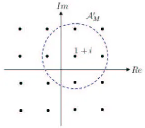
where p ∈ (0, 1) denotes a probability, A0
M is a subset of AM containing all neighbors
of a, and λ is a constant positive integer. In our work, A0
M is defined as all nearest
points of a. Taking a = 1 + i in 16-QAM for example, the region of A0
M is shown in
Figure 5.2. Even though a is not the global optimal point exactly, the true optimum may occur within its neighbors intuitively. Hence, higher probabilities are assigned to the four points nearest a and a itself.
Including these components into the updating of the CE-based MIMO detection method, the updating formula of importance distributions are revised as follows,
f(k+1)(xi = a) = α1fs(k)(xi = a) + α2fg(1)(k)(xi = a) + α3fp(1)(k)(xi = a) + Ã 1 − 3 X i=1 αi ! f(k)(x i = a), (5.12)
where αi are weighting factors with 0 ≤ αi < 1 for i = 1, 2, 3 and 3
X
i=1
αi < 1.
The algorithm of the Particle-Swarm-driven CE MIMO detection method is listed in Table 5.2. As shown in the simulations, the PS-driven CE MIMO detection method provides a significant improvement in the BER performance compared with the CE-based MIMO detection method.
Figure 5.2: An example of region of A0
M as a = 1 + i with 16-QAM.
Step 1 : Initialize the importance distributions f(k)(x
i) with uniform
distribution for i = 1, · · · , NT, respectively. And set k = 0.
Step 2 : Generate U samples xk
i,u from f(k)(xi) for u = 1, · · · , U .
Construct the set {xk
u}Uu=1 where xku = [x1,uk , · · · , xki,u, · · · , xkNT,u]
T.
Step 3 : Calculate the set of scores {S(xk
u)}Uu=1 according to equation (5.3).
Step 4 : Set a quantile parameter ρ such that there is a γk satisfying
equation (5.5).
Step 5 : Calculate the distribution of elite samples in accordance with equation (5.6).
Step 6 : Update the sample vector with the best score overall (from the 1st to the kth iteration), xk
g(1), and the best sample vector in the
current iteration, xk p(1).
Step 7 : Calculate the component importance distributions fg(1)(k) and fp(1)(k) according to equation (5.8) and (5.9).
Step 8 : Update the importance distributions following the revised updating equation (5.12).
Step 9 : Stop at iteration k = K if the pre-defined stopping criterion is met; otherwise, let k = k + 1 and go back to Step 2.
Table 5.2: The Particle-Swarm-driven CE MIMO detection algorithm.
As mention in the previous section, the weighting factors follow the rule of that in the CE-based MIMO detection method. The weighting for the distribution of the previous iteration remains most part of the updating equation.
5.3.2
Modifications for the PS-Driven CE Method
Enhancement of the effects of sample vectors in the current iteration and those among all iterations leads to a uniform convergence. However, it may encounter the problem of being trapped in a local minimum. To draw a higher probability to explore the global minimum during the procedure, the samples vectors with the second best score are also considered.
Let xg(2) and xp(2) denote the sample vectors with the second best score among all
iterations and in the current iteration, respectively. Similar to fg(1)(k)(xi) and fp(1)(k)(xi),
fg(2)(k)(xi) and fp(2)(k)(xi) are given depending on these two vectors. Including the two new
added distributions to the updating formula of importance distributions, equation (5.12) can be modified as f(k+1)(x i = a) = α1fs(k)(xi = a) + α2fg(1)(k)(xi = a) + α3fg(2)(k)(xi = a) +α4fp(1)(k)(xi = a) + α5fp(2)(k)(xi = a) + Ã 1 − 5 X i=1 αi ! f(k)(xi = a), (5.13)
According to equation(5.13), any one component can be dropped if the corresponding weighting factor is assigned to zero. Thus there are several combinations of the composite components for the updating formula. To further extend this model, the sample vector with the third best score can even be considered. However, the sample vector with too poor score will degrade the performance. Therefore, to enhance the exploration ability of this algorithm, the sample vectors used should have relatively better scores but not
too worse at all. The discussion of different combinations for those component is given in Chapter 6 with their BER performances.
5.4
Score Function under Imperfect Channel
Esti-mation
So far, the channel state information is assumed perfect known at the receiver. Thus the score function used in the proposed algorithms is defined as
f (x, y, H) = ||y − Hx||2.
Recalling a detector in the ML sense and define the likelihood function as L(y|H, x), the ML detector estimates x by maximizing the likelihood function under i.i.d. Gaussian noise: ˆ xM L = arg max x∈ANTM L(y|H, x) (5.14) = arg min x∈ANTM (− log L(y|H, x)) (5.15) = arg min x∈ANTM ||y − Hx||. (5.16)
However, when imperfect channel estimation is taken into account, the score function must be modified in the presence of channel estimation errors. Denote Lm(y| ˆH, x) the
modified likelihood function which is obtained by averaging L(y|H, x) over all estimation errors as [10] Lm(y| ˆH, x) = Z H∈CNR×NT L(y|H, x)p(H| ˆH)dH (5.17) = EH| ˆH h L(y|H, x)| ˆH i . (5.18) = CN (δ ˆHx, Σw+ δΣ∆H||x||2) (5.19)
as ˆ xM L = arg min x∈ANTM ³ − log Lm(y| ˆH, x) ´ (5.20) = arg min x∈ANTM NRlog π(σw2 + δσ∆H2 ||x||2) + ||y − δ ˆHx||2 σ2 w+ δσ2∆H||x||2 . (5.21)
Hence the modified score function in the presence of imperfect channel estimation is defined as fm(x, y, ˆH) , − log Lm(y| ˆH, x) (5.22) = ||y − δ ˆHx||2 σ2 w+ δσ∆H2 ||x||2 + NRlog π(σ2w+ δσ∆H2 ||x||2) . (5.23)
The first term in equation (5.23) is similar to the original score function. It also indicates that the modified score function only includes the term σ2
∆H instead of other detailed
Chapter 6
Simulation Results
In this chapter, we examine the performance of various proposed MIMO detectors. A MIMO system with NT = 4 transmit antennas and NR = 4 receive antennas with
4-QAM modulation is considered. Let Eb be the average received energy per information
bit and denote by N0 the noise power density. The signal-to-noise (SNR) ratio is defined
as Eb N0 = NR log2(M)σ2 w . (6.1)
6.1
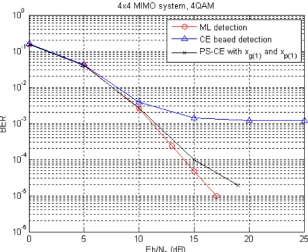
Perfect Channel Estimation
The channel matrix is assumed perfect known by the receiver in this section. Fig. 6.1 shows the bit error rate (BER) of the CE-based detection method with α = 0.3 and the PS-driven CE MIMO detection method with α1 = α2 = 0.1 ,α3 = 0.2 and β = 0.3.
It is obvious to see that the proposed PS-driven CE detection algorithm can effectively solve the problem of nonuniform convergence in the CE-based detection algorithm. The error floor caused by the CE-based detection is eliminated at high SNR regions.
The BER performance comparison between some existing detection methods such as ZF, MMSE, ZF-VBLAST and the PS-driven CE detection algorithm is shown in Fig. 6.2. Due to noise enhancement, the performance of ZF is poor in comparison to ML even with V-BLAST algorithm. MMSE offers a slight improvement compared with ZF.
Figure 6.1: BER performance of the two proposed detectors.
The proposed algorithm provides a near-ML performance and outperforms the MMSE detector by more than 12dB at BER=10−4.
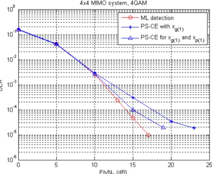
Next, we discuss some modifications for the PS-driven CE detection methods. BER performances are shown for the PS-driven CE detection method with different combina-tions in the updating formula, equation (5.13). Fig. 6.3 compares the difference between the one using xg(1) only and the one using both xg(1) and xp(1). As shown in this figure,
the one using both xg(1) and xp(1) reaches lower BER when SNR is larger than 10dB
since xp(1) provides another more reliable position at each iteration in addition to the
best position among overall iterations.
Figure 6.3: BER comparison of the PS-driven CE detector using(1) xg(1) only; (2) both
xg(1) and xp(1).
Although including the use of best sample vector in every iteration leads to an obvious improvement instead of using xg(1) only, it is possible that the swarm is trapped in a
local minimum since only the best sample vectors are considered. Replacing xp(1) with
methods.
Figure 6.4: BER comparison of the PS-driven CE detector using xg(1) and (1) xp(1); (2)
xp(2); (3) xp(3), respectively.
As expected, the one with xp(2) performs best among these three scenarios. The case
of xp(3)provides a similar contribution with that of xp(2). However, the third best sample
vector may be too far away the optimum and can’t afford good enough information. Fig. 6.5 shows results of adjustments for the weighting factor of xp(2). The weighting for
fg(1)(k)(xi) and fs(k)(xi) remain constant as 0.1, respectively. In Fig. 6.6, the combination
of xg(1), xg(2) and xp(2) is considered. It also indicates that the sample vectors used in
each iteration plays an more important role for the algorithm rather than those among all iterations.
Figs. 6.7 and 6.8 verify the one with xp(2) performs better than that with xp(1). Fig.
6.8 plots the averaged minimum distance trajectory, i.e. ||y − Hx||2, at each iteration
when SNR is 15 dB over 1,000,000 simulations and it exhibits that using xp(2) exactly
Figure 6.5: BER comparison of the PS-driven CE detector using xg(1) and xp(2) with
different weighting of xp(2).
Figure 6.6: BER comparison of the PS-driven CE detector using (1)xg(1) and xp(2);
Figure 6.7: Symbol error rate performance of the PS-driven CE detector using xg(1) and
(1) xp(1); (2) xp(2), respectively.
Finally, we present the BER performance using the PS-driven CE detection method which uses the components of xg(1) and xp(2) in a 6 × 6 MIMO system.
Figure 6.9: BER of a 6×6 MIMO system with 4-QAM under the PS-driven CE detection algorithm and ML detection.
6.2
Imperfect Channel Estimation
In this section, the channel estimation error is included. Orthogonal training se-quences are generated from a perfect root-of-unity sequence (PRUS) [16] which can be constructed by the Frank-Zadoff-Chu-sequence [17] as
s(k) =
½
ejπCk2/N
, for N is even
ejπCk(k+1)/N, for N is odd (6.2)
with k = 0, · · · , N −1 where N denotes the length of sequence and C is a positive integer that is coprime to N. The updating formula for importance distributions is chosen to
be
f(k+1)(x
i = a) = 0.1fs(k)(xi = a) + 0.1fg(1)(k)(xi = a)
+0.2fp(2)(k)(xi = a) + 0.6f(k)(xi = a) (6.3)
since it performs best according to the simulation results shown in the previous section. Fig. 6.10 shows the BER performance with σ2
∆H = 0.03 and NP = 8 using the original
score function and the modified one.
Figure 6.10: BER performance comparison of a 4 × 4 MIMO system with 4-QAM based on different score functions with σ2
∆H= 0.03.
6.3
Complexity Comparison
The computational complexity comparison of conventional detectors and the pro-posed detectors is listed in Table 6.1.
Although the complexity of the proposed detectors is higher than conventional de-tectors such as ZF, MMSE, ZF-VBLAST, the BER performance of the PSD-CE outper-forms those detectors. Compared with the ML detector, the complexity is much lower
when NT is large. Though the sample size U increases as the constellation size M
in-creases, it has a very slight variation while NT increases. Taking 4 × 4 and 6 × 6 MIMO
systems for example, the complexity of the PSD-CE detector for these two cases is the same since U and Nitr remain constant in the two cases. However, the complexity of
ML detector increase two orders when the number of antennas is raised from 4 to 6.
Detector Complexity ML (NTNR+ NR) × MNT ZF 4N3 T + 2NT2NR+ NTNR MMSE 4N3 T + 2NT2NR+ NTNR+ NT ZF-VBLAST NT X i=0 (4i3+ 2N Ri2) + NXT−1 i=0 [NT(NT − i) + 2NT] CE [(NTNR+ NR) × U + 3] × Nitr PSD-CE [(NTNR+ NR) × U + 5] × Nitr
Chapter 7
Conclusion
The purpose of this thesis is to present alternative algorithms for detecting signals in a MIMO system. We first propose a detector which is based on the Cross-Entropy (CE) method. The CE-based MIMO detection method is a Monte-Carlo based approach to estimate the importance distribution of transmit signals by minimizing the distance be-tween the provisional distribution derived at each iteration and the optimal importance distribution. Simulation result indicates that the BER performance of our detector is close to the ML detector when SNR is comparatively low. However, an error floor occurs at high SNR region due to nonuniform convergence of the CE approach.
To improve the CE-based MIMO detector and reduce the error floor, we include the ideas of the Particle Swarm Optimization (PSO) and propose the PS-driven CE detection algorithm. Updating the importance distributions by a mixture of densities determined by the elite set and the best sample vector among all iterations improves the detector performance. In addition, considering the best sample vector at each iteration in determining the updated importance distributions further improves the performance. Moreover, to extend the PS-driven CE MIMO detection algorithm, some modifications for the updating formula of importance distributions are also considered. As shown in the simulation results, PS aided CE approach can significantly eliminate the error floor, outperforming the conventional ZF or MMSE detector by more than 12dB at BER=10−4.
To take into account the channel estimation errors, we propose a robust detector structure which is based a modified score function. The estimation errors are modelled as complex Gaussian distributed and the modified score function includes the variance of the channel estimation error as an extra term. Simulation results prove that the modified score function used by our detector helps to improve the BER performance when the practical imperfect channel estimation scenario is considered.
Bibliography
[1] D. Tse and P. Viswanath, Fundamentals of Wireless Communication, Cambridge University Press, 2005.
[2] E. Biglieri, R. Calderbank, A. Constantinides, A. Goldsmith, A. Paulraj and H. V. Poor, MIMO wireless communications, Cambridge University Press, 2007.
[3] J. Kennedy and R. C. Eberhart, “Particle swarm optimization”, Proc. of the IEEE
Int. Joint Conf. on Neural Networks, pp. 1942-1948, 1995.
[4] A. P. Engelbrecht, Fundamentals of Computational Swarm Intelligence, John Wiley & Sons, 2005.
[5] F. Heppner and U. Grenander, “A stochastic nonlinear model for coordinated bird flocks”, S. Krasner, editor, The Ubiquity of Chaos, AAAS Publications, Washington, DC, 1990.
[6] J. N. Kapur and H. K. Kesavan, Entropy Optimization Priciples with Applications, Academic Press, New York, 1992.
[7] R. Y. Rubinstein, “Optimization of computer simulation models with rare events”,
European Journal of Operational Research, vol.99, pp. 89-112, Nov. 1997.
[8] R. Y. Rubinstein, “The cross-entropy method for combinatorial and continuous op-timization”, Methodology and Computing an Applied Probability, vol.2, pp.127-190, 1999.
[9] R. Y. Rubinstein and D. P. Kroese, The Cross-Entropy Method, Springer, 2004. [10] S. M. S. Sadough, M. A. Khalighi, and P. Duhamel, “Improved iterative MIMO
signal detection accounting for channel estimation errors,” IEEE Trans. on Vehicular Technology, accepted for future publication.
[11] G. H. Golub and C. F. Van Loan, Matrix Computations, Johns Hopkins University Press, Baltimore, MD, 1983.
[12] P. W. Wolniansky, G. J. Foschini, G. D. Golden and R. A. Valenzuela, “V-BLAST: An architecture for realizing very high data rates over the rich-scattering wire-less channel,” Proc. of IEEE Int. Symposium on Signals, Systems and Electronics
(ISSSE’98), Pisa, Italy, Sep. 1998.
[13] A. A. Khan, M. Naeem and S. I. Shah, “A particle swarm algorithm for symbols detection in wideband spatial multiplexing systems,” Proc. of the Genetic and
Evo-lutionary Computation Conf. (GECCO’2007), London, U. K., pp. 63-70, Jul. 2007.
[14] J. Kennedy and R. C. Eberhart, Swarm Intelligence, Morgan Kaufman publisher, 2001.
[15] J. Kennedy and R. C. Eberhart, “A discrete binary version of the particle swarm algorithm,” IEEE Int. Conf. on Systems, Man, and Cybernetics, pp.4104-4108, 1997. [16] O. Weikert, U. Z¨olzer, “Efficient MIMO channel estimation with optimal training sequences,” Proc. of 1st Workshop on Commercial MIMO-Components and-Systems
(CMCS 2007), Duisburg, Germany, Sep. 2007.
[17] D.C. CHu, “Polyphase codes with good periodic correlation properties,” IEEE
1985
Graduate Courses
1. Coding Theory
2. Computer Communication Networks (I) 3. Detection and Estimation Theory
4. Digital Communications 5. Digital Signal Processing 6. Matrix Computation
7. Multimedia Communications 8. Stochastic Processes
![Figure 2.1: A MIMO system model. where x = [x 1 , · · · , x N T ] T ∈ A N M T , (2.2) y = [y 1 , · · · , y N R ] T ∈ C N R , (2.3) w = [w 1 , · · · , w N R ] T ∈ C N R , (2.4) H = h 1,1 · · · h 1,N T ..](https://thumb-ap.123doks.com/thumbv2/9libinfo/8634151.192663/17.892.137.812.128.787/figure-mimo-model-t-r-h-n-t.webp)