Minimax Design of Low-Delay Perfect-Reconstruction FIR Filter Banks

Minimax design of two-channel low-delay

perfect-reconstruction

FIR

filter banks

S

.-J

.

Ya n g J.-H.Lee B.-C.Chieu

Abstract: The authors deal with the design

problem of low-delay perfect-reconstruction filter banks for which the FIR analysis and synthesis filters have equiripple magnitude response. Based on the minimax error criterion, the design problem is formulated in such a manner that the coefficients for the FIR analysis filters can be found by minimising the weighted peak error of the designed analysis filters, subject to the perfect- reconstruction constraints. A design technique based on a modified dual-affine scaling variant of Karmarkar’s algorithm, in conjunction with approximation schemes, is then developed for solving the resulting nonlinear optimisation problem. The effectiveness of the proposed design technique is demonstrated by several simulation examples.

1 Introduction

Filter banks have been widely used in the areas of sub- band coding of speech signals [l], image signals [2, 31 and transmultiplexing [4]. A filter bank having a perfect-reconstruction property can provide a reconstructed signal that is exactly a delayed replica of the input signal, without introducing reconstruction error.

In the literature, several techniques have been pro- posed for the design of two-channel perfect-reconstruc- tion (PR) linear-phase (LP) FIR filter banks [5-81. In general, the overall system delay of an LP FIR filter bank is totally determined by the lengths of the FIR fil- ters used. Although a filter bank with two channels is very useful for tree-structured sub-band coding of speech signals [9] and wavelet transform [lo], the inher- ent, long system delay, caused by using the two-channel PR LP FIR filter banks designed using the techniques of [5-81, may make the overall system objectionable in practical implementations and applications of sub-band coders. However, the overall system delay of a tree- structured sub-band system can be significantly reduced 0 IEE, 1999

IEE Proceedings online no. 19990179 Dol: 10.1049/ip-vis:19990179

Paper first received 23rd February and in revised form 29th June 1998 J.-H. Lee is with the Department of Electrical Engineering, National Taiwan University, Taipei 106, Taiwan

S.-J. Yang and B.-C. Chieu are with the Department of Electronic Engineering and Technology, National Taiwan Institute of Technology, Taipei 106, Taiwan

by imposing low reconstruction delay on splitting stages located deep inside the tree.

A filter bank with low reconstruction delay and filter length N has a system delay of k,, which is less than N

- 1 [ll]. Recently, many techniques have been pre- sented for designing two-channel low-delay filter banks [I 1, 121. The time-domain technique of [Ill can design an FIR filter bank with adjustable reconstruction delay. However, the output signal-to-reconstruction noise ratio SNR, of the designed filter bank is unsatis- factorily low.

Two techniques have been presented in [ 121 for designing two-channel low-delay PR FIR filter banks optimally in the least-squares sense. Although design- ing a filter bank that has analysis and synthesis filters with frequency responses that are optimum in the least- squares sense is a popular task and is useful for sepa- rating the channels in communication systems [13], the maximum ripple of the frequency responses of the designed analysis and synthesis filters may not be as small as possible. Moreover, our experience shows that designing filters with equiripple response (i.e. optimum in the minimax sense) generally results in the advantage of smaller error ripple than that with least-squares response at the same filter length. Therefore it is worth investigating the problem of designing low-delay per- fect-reconstruction filter banks that have FIR analysis and synthesis filters with equiripple magnitude response. However, the resulting design problem is, in general, a highly nonlinear optimisation problem that is difficult to solve. As to the design method of [16], which is based on the least-squares optimum criterion, the PR constraints cannot be guaranteed during the design process.

In this paper, we present a technique based on a modified dual-affine scaling (MDAS) variant of Kar- markar’s algorithm proposed in [14], in conjunction with approximation schemes for solving the considered design problem. The design problem is first formulated as a minimax optimisation problem, with two sets of nonlinear constraints for the responses of analysis fil- ters and for the conditions of perfect reconstruction, respectively. Approximation schemes are proposed to simplify these two sets of nonlinear constraints. Then, we utilise the MDAS variant of Karmarkar’s algorithm of [I41 to solve the resulting linearly constrained mini- max optimisation problem.

2 Low-delay perfect-reconstruction FIR filter banks

Fig. 1 shows the basic structure of a two-channel filter bank. The low-pass and high-pass analysis filters are designated by Ho(z) and H , ( z ) , respectively, and the 15 IEE Proc.-Vis. Image Signal Process., Vol. 146, No. I , Frbruar?, 1999

low-pass and high-pass synthesis filters are designated by F,(=) and F l ( z ) , respectively. It is well known that the input-output relationship in the 2 transform is given by

(1) The first term of eqn. 1 represents a linear shift-invari- ant system response, which is the desired signal transla- tion from x(n) to

.?(n),

and the second term represents the aliasing error due to the change of sampling rate in the filter bank. Setting the synthesis filters F o p ) , =

2H1(-z) and F I ( z ) = -2Ho(-z) eliminates the aliasing term. Hence, eqn. 1 becomes

X ( z ) = T ( z ) X ( z ) (2)

(3)

where

T ( z ) =

[Ho(z)H1(-4

- H1(4Ho(-z)l 2.

I

Conditions for low-dela y perfect- reconstruction

Eqn. 2 reveals that producing a reconstructed signal i ( n ) that is a delayed replica of x(n) (i.e. perfect recon- struction) requires

Ho(z)Hl(-z)

-

Hl(z)Ho(-z)

= bz-'" (4)

where b is a positive constant, and kd represents the system delay. Let the lengths of the analysis filters

Ho(z) and H l ( z ) be No and N I , respectively. For low delay, k,/ must be a positive odd integer less than ( N o

+

N 1 ) / 2 - 1 [ l l , 121. Let h = 1 for simplicity. From eqn. 4, conditions for perfect reconstruction can be expressed as follows [12]: 1 2 23-1 (-l)"o(23

-

1 - IC)hl(IC) = - S ( j - k')

(5)

k = O or 1 2 23-1 - _{(-1)'h1(23 - 1 -}

_k)ho(k)

_{= -6(3 - IC') (6)} f o r j = 1, 2, ..., N,, where k' = (kd+1)/2, 6(x) = 1 , only when

x

= 0, and = 0, else.

+ N 1 - 1

N , =

{

0 2

k =Q

if NO + N I is even if

NO

+

N I

is odd In matrix form, eqns. 5 and 6 can be rewritten as

(7) 1

2 (-l)zMthl-t = -m

for i = 0, 1, where M, is an N , x N I - , matrix with entries given by

( M t ) j , k = (-1)"'h,(2.1 - k ) ( 8 )

for j = 1 , 2,

...,

N,, and k = 1, 2, ..., N I _ , . Note that some entries of M,, namely, when k > 2,, are zero. m is

16

an N , x 1 column vector given by

m = [ r n l m a

. . -

rnk'

. . .

7n,y

1'

(9) with 1 if j = k' 0 i f j # k ' ribJ = and h, = [h,(O)

h,(l)

. . .

h,(N, - l) I T (10) for i = 0. 1, a n d j = 1, 2, ..., N , . Eqn. 7 can be rewritten in an equivalent form as follows:

U,h = m

where

(11)

U , = [ - M 1 Mol (12)

and

2.2 Desired responses for analysis filters To achieve the design of PR FIR filter banks with a preset system delay kd, we have to investigate the desired frequency responses for the FIR analysis filters. Let the Fourier transform for each of the desired anal- ysis filters be D,(do), i = 0, 1, and let the constant group dellay for each of the desired analysis filters be k,, i = 0, 1, in the passband. Then, the desired frequency responses D,(d@) can be expressed as

D , ( p ) = & f ( + - - 3 ( w k z + Q 2 (14) for i = 0, 1, where M,(o) 2 0 and 0, are the desired magnitude responses and the constant phases, respec- tively. Also, k , < ( N , - 1)/2. As h,(n) are real-valued, it is clear that M,(-u) = M I ( @ , and 0, = m,r, for i = 0, 1, where m, are integers. Substituting eqn. 14 into eqn. 3

yields

= D o ( e J W ) D 1 ( e ~ ( ~ + ~ ) ) - ~1 ( e ~ ~ ) ~ ~ ( c ' ( ~ + ~ ) )

(15)

As Ho(z) and H l ( z ) are low-pass and high-pass filters, respectively, the corresponding desired frequency responses Do(e'@) and Ill(@') must be the ideal low-pass and high-pass filters, respectively. Therefore the second term of the right-hand side of eqn. 15 is negligible com- pared with the first term in the low-frequency band. Thus, we have the following approximation:

TO

( )

M ~ ( ~ ) M ~

+ n ) e - 3 ( w k o + B o ) e - ~ ( w k i + Q i + k i n ) (16) in the low-frequency band. From eqns. 4 and 16, it fol- lows that

M ~ ( ~ ) A ~ ~ ( ~

+ ~ ) e - 3 [ w ( k o + k l ) + Q ~ ~ + ~ l + k l n ] e 3 w k d (17) in the low-frequency band. It is obvious from eqn. 17 that ko

+

k I = k d must be an odd integer, and 0,, for i = 0, 1, must be chosen to satisfy

(18) if kl is even

Bo

t-

81 =

{

:E-

1)n if kl is odd

where rn is an integer. Similarly, it can be derived that

Oi,

for i = 0, 1, must be chosen to satisfy

(19)

{En-

1). if ko is even

if is odd

Bo

+

81 =

in the high-frequency band, where n is an integer. Based on the above results, we can set

eo

= 0 for sim- plicity. Accordingly, we obtain from eqn. 14 that the desired frequency responses for Ho(z) and H , ( z ) are given by

and

Do(&") = Mo(w)e-jwko (20)

MI

(w)e-jwkl if k1 is even

D1(e'") =

{

M1(w)e-j("kl+a) if

k1

is odd (21)

respectively.

3 Formulation of design problem

Here, we consider the minimax design problem of the low-delay two-channel PR FIR filter banks as shown in Fig. 1. Let the Fourier transform for each hi(n), i = 0, 1, be Hi(d"). The corresponding error between Di(e'") and the designed response

Hi(@)

is defined as

E;(.+)

= Di(ej") - Hi(e+) ₍₂₂₎ for i = 0, 1. The problem of optimally designing a low- delay PR FIR filter bank in the minimax sense is to design Hi(@)) such that the weighted peak ripple of Ei(dw) is minimised, subject to eqn. 7, for low-delay perfect reconstruction. Hence, the design problem can be formulated as

minimise ~ ~ W ~ ( w ) E t ( e ~ w ) ~ ~ m subject to

U,h

= m

for i = 0 , 1

(23)

where I(x(1, denotes the L, norm of x, and W,(U)) denotes the weighting function. Eqn. 23 can be rewrit- ten in an equivalent form as follows:

minimise 6, 6

2

0 subject to

Wi(w)lDi(ejw)

- Hi(e+)I

5

6 U,h = m for i = O , 1 (24)

{

As both Di(d") and Ei(d") are, in general, complex- valued, the design problem shown by eqn. 24 can be further rewritten in an equivalent form as follows:

minimise E , E

>_

0 subject to

o

5

W , " ( w ) ( D i ( e j w ) - H ; ( e j " ) l 2

5

e U,h = m for i = O , I (25)

c

for i = 0, 1, where E =

B.

From eqn. 25, we note that the resulting design prob- lem contains two groups

of

nonlinear constraints. The first group contains a set of nonlinear inequalities rep- resenting the squared weighted error between the desired and designed frequency responses of the analy- sis filters. The second group, leading to N , nonlinear equations, represents the conditions required for achieving perfect reconstruction. Therefore, solving the optimisation problem of eqn. 25 directly by employing conventional nonlinear programming techniques is not IEE Pro,.-Vis. Imuge Signal Process., Vol. 146. No. 1. Februury 1999

an efficient method. In the following Section, we present an effective technique based on a linear-pro- gramming algorithm in conjunction with approxima- tion schemes to solve eqn. 25.

4 Proposed design technique

Let hor and h,' be the coefficient vectors and Hor(e'") and Hlr(e'") be the corresponding frequency responses of the analysis filters computed at the rth iteration during the optimisation process. Moreover, assume that AH,'(e'") represents the deviation for H,'(d") corresponding to the perturbation Ah,' = [Ah,'(O) Ahlr( 1)

...

Ah,'(N, - l)lT performed on h,' at the rth iteration for i = 0, 1. As a result, the constraints for the frequency responses of the analysis filters in eqn. 25 can be reformulated as

o

5

~ , ( u )

{

IDt(e3u) - HT(e'u)12

- 2Re

{

[Dt(e3") -

H,'(e3")]*

h H , ' ( e 3 " ) }

(26) where the superscript * denotes a conjugate operation. Assume that the perturbation Ah,' performed on h,' is sufficiently small at each iteration. Then, the term

lAH;(d")(* in eqn. 26 can be neglected. Therefore, eqn. 26 can be approximated by the following expres- sion:

o

5

~ ~ ' ( w )

{

l D t ( e j w ) - "( e j i J ) I 2 -2Re

{

[ D z ( e j w ) -

H,'(e3")]* A H : ( e J " ) } }

- < € (27) With this approximation scheme, the design problem of eqn. 25 becomes

minimise E , E

>_

0

subject to

o

5

~ : ( w >

lDt(eJu) - H ; ( P J ) ~ ~

-2Re

{

[Dz(eJ'") - H:(eJ")]* A H T ( e J " ) }

}

5

E

{

U,h = m

From eqn. 28, we note that the PR constraint U,h = m

applies to both the original vector h' and the perturbed version h'

+

A h ' .

Let Q = {q,,

wl,

..., mK-l}

be a dense grid of frequen- cies linearly distributed in the range from U ) = 0 to U ) =

n

for evaluating the frequency responses and the

related error functions. Next, we construct several use- ful matrices as follows:

where 0 denotes a matrix with appropriate size and zero entries. WO and W , are two submatrices with appropriate size, given by

WO= diag (\VO(WO)

. ..

M ~ & J & l ) )

and W1 = diag (Wl ( w o )

_.

.

.

Wl ( w K - - ~ ) )

(30)

respectively, where diug(*) denotes a diagonal matrix.

where U. and U I are two submatrices with the (k, 0th entry given by

(32)

(uz)k,l

= e - J u L - l ( l - l )

for i = 0, 1, k = 1, 2,

...,

K , and 1 = 1, 2, ...,

NP

d =

I

[::

( 3 3 )

where do and dl are two vectors given by

-

-where ce0 and cel are two vectors with the kth entry given by

( c e z ) k = w , ( w ~ C - ~ ) IDZ(eJuL-1) - H l ( e J W L - 1

)I2

(37) for i = 0, 1, and k = 1, 2,

...,

K , at the rth iteration. Accordingly, eqn. 27 can be rewritten as

(38) where 1 and 0 represent the column vectors with appropriate size and all entries equal to 1 and 0, respectively. To simplify eqn. 28, we further construct the following matrices:

0

5

c , - 2W'Re {[diag(e)]*U} Ah'

5

E . 1

P

= 2 W 2 R e { [ d i a g ( e ) ] * U } (39)

-P

-1

A = [ p

0 1

(43) ~I

In matrix form, the design problem shown by eqn. 28 can be expressed in the form of a dual optimisation problem, as follows:

maximise bT

w

ATw

L c U,h = m

subject t o (44)

To maximise bTw while satisfying both of the con- straints in eqn. 44, the coefficient vector h is parti- tioned into two components as follows:

h = h,

+

h,

where h, denotes a vector in the null subspace of U,,

and h,. denotes a vector in the subspace that is orthogo- (45)

18

nal to the null subspace of Ur. Accordingly, the pertur- bation performed on the coefficient vector at the rth iteration can be written as

Ah'

= Ah;

+

Ah:

₍₄₆₎

where Ahnr is a perturbation vector in the null subspace of Uc, and Ah; is a perturbation vector in the subspace orthogonal to the null subspace of U,. Substituting eqn. 46 into w of eqn. 41 yields

where

w=w,+w,

(47)

We note from eqn. 25 that there are only N,, = ( N o

+

N , ) - N,. degrees of freedom available for finding the optimum coefficients for the analysis filters, owing to the perfect-reconstruction constraints. Hence, it is appropriate to solve the constrained optimisation prob- lem by using the component Ah,' to find the optimum filter coefficients and using the component Ah; to sat- isfy the perfect-reconstruction constraints. Substituting eqn. 47 into eqn. 44 yields an equivalent problem as follows: maximise bT(w,

+

w,)

(49)

AT@,

+

w,)

I

c U,h = m subject t o 4.

I

programming

To ensure the requirement that the component Ah/ must be in the null subspace of U, during the design process, we propose an appropriate method for finding

w,

as follows. Consider the operator I-U, T(U,U,7)-'U,

for projecting a vector onto the null subspace of U,, where I is the identity matrix with appropriate size. Performing the eigen-decomposition for the projection operator, we can express it as follows:

where

Determining Ahnr using linear

I

-

u ~ ( u , u ~ ) - ~ u ,

= Q A Q ~ ₍₅₀₎

Q =

[ S I 9 2 . ' . q N n ]

O 1

rxl

o

. . -

(51)

[

0

.o.

. ' .

0 AN,, O

J

where AI 2 A2 2

...

2 AN,, > 0 are the eigenvalues of the projection operator in descending order, and qr, i = 1,

2, ..., N,,, are the corresponding eigenvectors. Hence, the set of eigenvectors given by {ql q2 ... q N , } forms a basis that spans the null space of

U,. As

the component Ahnr lies in the null space, it can thus be expressed as a linear cornbination of {q, q2

...

qN,} as follows: where x denotes the coefficient vector for this linear combination. Substituting eqn. 52 into w,,, which is given by eqn. 48, and performing some algebraic manipulations, we obtain

where

Ah; = QX (52)

w,

=

Br

(53)

.=[:

PI

(54)

(55) Based on the dual-affine scaling variant of Kar- markar's algorithm presented in [ 141, we introduce slack variables to the formulation of eqn. 49 and use eqn. 53. This leads to the following constrained optimi- sation problem, which is equivalent to eqn. 49:

maximise bT(Br

+

w,)

subject t o

{

A T B r + w , ) + v = c , ( U,h, = m

v > O

(56) where v is the vector containing the slack variables.

Next, assume that we have an interior feasible solu- tion WO = Bro

+

:w that satisfies AT(Bro

+

):w

+

vo = c

and vo > 0 at the initial stage. With the initial solutions

ro and vo it has been shown in [15] that an appropriate scaling operation must be performed to update r and v such that the objective function bT(Br

+

w,) can be improved at a faster rate. In [14], it was proposed to scale the slack variables as follows. During each itera- tion, we first define

G = D i l v ( 5 7 )

D,

= diag(v) (58)

where

Substituting eqn. 57 into eqn. 56, we obtain maximise bT(Br

+

w,)

T B r + w c ) + D , G = c , G > O

subject t o { A (

U,h, = m

(59) Let the feasible solutions for eqn. 56 be given by

S

= {r E RN"+'IAT(Br

+

w,)

5

c } Then, the set of feasible scaled slack vectors for eqn. 59 is given by

V = { G E R4K13r E S, AT(Br

+

w,)

+

D,G = c } It follows from eqn. 59 that the corresponding r in S

for a given B in V is given by

r(+) = ( B T A D ; ~ A T B ) - ~ B T A D ; ~

(60) and the one-to-one relatiopship between the feasible directions f,. in S and f,- in V is given by

x

( D l ' c

- G - DLIATw,)

fc = -DtlATBf, (61)

Eqn. 60 reveals that the Moore-Penrose pseudo-inverse of the matrix D;'ATB is employed to solve the associ- ated overdetermined linear equation system. Based on eqns. 59 and 60, the feasible direction fG can be obtained by computing the gradient of the objective function br(Br

+

w,) with respect to B, as follows:

fc = VO (bT(Br(G)

+

w,))

= - D i l A T B (BTADi2ATB)-l BTb

(62) Comparing eqns. 61 and 62, we obtain

f, = (BTADL2ATB)-' BTb (63)

IEE Proc.-Vis. Image Signal Process.. Vol. 146, No. I , Februury I999

After determining f,. from eqn. 63, we note that Ah; can be obtained as follows:

Ah: =

Q ( x r

+

a f z ) (64)

if a suitable step size cc is found, where x' represents the

x obtained at the rth iteration during the optimisation process. The f, of eqn. 64 is the subvector containing the first N , entries of the feasible direction f,. We use this f, as the true descent direction for updating the coefficient vector x of the optimisation problem in eqn. 59. To find a suitable step size

a

for obtaining

Ah; analytically instead of numerically, we propose a simple and efficient method by considering the feasibil- ity of using the updated slack variable v'

+

af,.

First, from eqns. 57 and 62, we have the feasible direction for the unscaled slack variable as follows:

f, = -ATB (B"ADi2ATB)-' BTb = -ATBf,

Then, based on the fact that the updated slack variable

v must be a vector with all entries greater than or equal to zero, a suitable step size

a

can be obtained by taking the most appropriate feasible step in the direction o f f , as follows:

(65)

where 0 < y < 1 is chosen experimentally. ( z ) ~ denotes the jth entry of the vector z, and min{x} denotes the minimum value of x. From eqns. 45 and 46, the for- mula for updating h, is given by

h;'" = h i

+

Ah: _{( 6 7 )} where h,' represents h, after the (r - 1)th iteration.

4.2 Determining Ah: using an approximation scheme

Here, the determination of the component Ah/ is con- sidered. Utilising eqns. 8, 12 and 67, U,. and h are first updated during the rth iteration. Let the updated results be denoted as U;:' and h;+', respectively. Next, assume that the increment obtained for updating h,. is

Ah: during the rth iteration. The corresponding incre- ment for updating U::' is designated as AU:c. Then, we take the maximum feasible increments for obtaining the results after the rth iteration as follows:

u;+1

= U;;'

+ nu;,

=

[

-

(MY:'

+

AM;,)

(NI;:'

+

AM;;,) ]

(68) and

hr+'

= ':h:

+

Ah;

=

[

(h;:'

+

Ah$

(hi:'

+

Ah;,)']'

(69) respectively, where AM&, AM[,, Ah& and Ah[, repre- sent the corresponding increments due to Ah,'. Moreo- ver, M6i1, M{:', h,',+' and hi:' represent the updated results for Mi;, Mi', hi; and h i , respectively, owing to the increment obtained from eqn. 64 for h, during the rth iteration. After the rth iteration, perfect reconstruc- tion requires

(70) U:+1h'f1 =

Next, substituting eqns. 68 and 69 into eqn. 70 yields

U',f'h'+'

=

UE:lhk+l -

AM?

hr+l

I C 071

+

Mg;lAh;,

-

MT:'AhG,

+

AM&hT;'

-

AMy,Ah&

+

AMg,Ahy, = m (71)

Let the,jth entry of the term AM[,h6inf' be denoted by

(AM;;. hbi,:'). From eqns. 8 and 10, it is easy to show that (AM,';.hhi')j is given by

(.1MT,h;:')j

23 =

C(-l)k+lahy,(zj

-

k)h&y(k

- 1) k = l 2 j =

C(-l)zj--m+2Ahr

I C ( 771 - l ) h 3 ; ; 3 2 j - r n ) m = l 2 j = - _{( - 1 ) m + l h ; 5 2 j} - m)OhTc(m - 1) m = l = -

(M;:lAhyC)j

for j = 1, 2,

...,

N,.. Hence, we have AM[,h6i1 =

-MbiIAh[,.. Similarly, it can also be shown that

AM& h[;l = -Mi:' Ah&. Accordingly, eqn. 71 can be rewritten as

U;+lhrfl

=

U;,flh;++l

+

2u;,f1Ah,T

= m (72)

Further, neglecting the second-order term of eqn. 72 provides an approximation expression as follows:

(73)

U,, r + l h, r + l

+

2U::lAhz

M in

Eqn. 73 leads to an appropriate approximation of the desired increment Ah; given by

Ah;

L(u~:~)T

( u ~ ; ~ ( u F : ~ ) T ) - ~

(m

-

U,, T + l h r + l

2

(74) for updating the component h, during the rth iteration to satisfy the constraints of perfect reconstruction. Note that the Moore-Penrose pseudo-inverse is used again to obtain eqn. 74 from eqn. 73. Taking the maxi- mum feasible direction for updating h,, we obtain the corresponding updating formula for h, as follows:

h,"'

=

hz

+

Ah; ₍₇₅₎ Hence. the updating formula for the coefficient vector

h after the rth iteration becomes

( 7 6 ) hrfl =

h;++'

+

h,'+1

4.3 Design procedure

We summarise the proposed design technique by pre- senting the following design procedure:

Step 1: Initialise the design process.

1. I : Construct the matrices W, U and d using eqns. 29,

31 and 33, respectively.

1.2: Select a suitable initial guess ho for h and set the iteration number r = 0. Our design experience shows 20

that an appropriate selection for h0 can be the uncon- strained least-squares solution given by ho =

{ Re[UHW2U]}-l Re[UHW2d], where U" denotes the Hermitian of U.

1.3: Cornpute the squared peak error ripple

8

corre- sponding to ho. Construct U> and m using eqns. 12 and 9, respectively. Moreover, find the matrix Q corre- sponding to U,'.

Step 2: At the rth iteration, set Ahn' = 0 and Ahcr = 0. Construct the matrix Q corresponding to the current coefficient vector hr. Then, calculate the corresponding error vector e' = d ~ Uh", the squared weighted error

vector c,' = W2[diug(er)]*(er) and the squared peak error ripple .C = 1.001 max{lcll}. Also, construct the matri- ces P and A using eqns. 39 and 40, respectively. Step 3: Eind the slack vector

where v1 = E'1 - c/, v2 = c l .

Step 4: Compute the feasible direction vector f, =

(BTAD;:!ATB)-'B% for optimisation. Instead of directly computing f,. by performing the inverse of

(B~AD,-;!A%), we propose an efficient procedure as follows:

4.1: Construct the diagonal matrices D , = diug(v1) and

D2 = diug(v2).

4.2: Compute the diagonal matrix D = (D1-2

+

D z - ~ ) .

4.3: Compute the column vector x1 = QTQI-21.

4.4: Compute the value cl = -(l%l)-I.

4.5: Solve the equation ( Q T Q P Q + cIxIxIT) f, =

-cIxI, using Gaussian elimination to find f,. 4.6: Compute the valuef, = cI(xITfr

+

1). 4.7: Form the desired direction vector

fr =

[

51

Step 5: Compute the feasible direction vector

f, = -ATBfr =

[

where f,,l =f,l

+

PQf,, and fv2 = -PQf,.

Step 6: Determine the step size a according to eqn. 66 and update the filter coefficient vector h as follows:

h,'+l = h"

+

aQf, according to eqn. 52. Construct the matrix U;:;' corresponding to h;+l

.

Step 7: Compute the increment vector Ah; using eqn. 74.

Step 8: Update the filter coefficient vector h as follows

h'+l h/'l

+

Ah;.

Step 9: Compute the squared peak error ripple &"+I

corresponding to hr+l. Construct the matrix Ucr+l cor- responding to hr+l.

Step 10: Define a performance indication function E(r

+

1) = ](E' ~- E ' + ~ ) / E ' ~ and a perfect-reconstruction indica- tion function z9(r

+

1) = max{lm - U;+lh'+ll}. It is rea- sonable to terminate the design process whenever the indication functions are small enough. Therefore we stop the iteration procedure if E(r

+

1) 5 K and 29(r

+

1) 5

q,

where K and q, are two preset small positive real numbers. Otherwise, set r = r

+

1 and go to step 2.

stopband ripple (PSR), defined as follows:

P P R = max

{

(Di(ej'") - H i ( e j " )

I}

for w E O p t

(77)

( 7 8 )

and

P S R = max

{

lDz(eju) - H i ( e + ) l } for w E R , ~ for each of Ho(e'") and Hl(ejm), where Qpr and Q.yi repre-

sent the passband and stopband of the analysis filter

Hi(&"), respectively. The weighting function

Wi(

w) used in eqn. 25 is set to Wp, and WYi for w E Qp, a.nd w E

respectively. In the transition band, W,(w) is set to

Wli. Moreover, the passband cutoff frequencies for

Ho(e/") and H I ( @ ) are

wpo

and

wpl,

respectively, and the stopband cutoff frequencies for Ho(e'") and HI(&") are q0 and

wsl,

respectively.

Example I : This example is the same as example 1 in [12]. We use the same specifications for this design: a low-delay system with No = 28, N I = 36,

wpo

= 0.49rc,

q0 = OAK, ko = 6 ,

wpl

= 0.6rc, ql = 0.4rc, k l = 9. The weights are set to Wpo = 2, W,,, = 6, W,, = W,, = 1, and W,, = W,, = 0. The values of 3: and q are set to 0.1, and respectively. The design process converges after 449 iterations, and we obtain the filter coefficients listed in Table 1 for the designed Ho(z) and

H l ( z ) . Table 2 shows the significant design results,

namely the PPRs and PSRs obtained using the pro- posed technique and the technique proposed by [ 121 for comparison. Clearly, the proposed design technique produces a better performance than the design tech- nique of [ 121.

The corresponding magnitude responses of Ho(z) and H l ( z ) are depicted in Fig. 2, and the corresponding group delays of Ho(z) and H l ( z ) are depicted in Figs. 3 and 4, respectively. Moreover, the resulting magnitude response and delay characteristic of T(z) are shown in Figs. 5 and 6, respectively.

5 Simulation examples

In this Section, we present several simulation examples of designing low-delay two-channel perfect-reconstruc- tion FIR filter banks for illustration and comparison. These designs are performed on a personal computer with a Pentium CPU, using MATLAB programming language. The performance for each of the designed low-pass and high-pass analysis filters is evaluated in terms of the peak passband ripple (PPR) and the peak Table 1: Coefficients of designed analysis filters for example 1 n ho(n) hl ( n) 0 1 2 3 4 5 6 7 8 9 10 11 12 13 14 15 16 17 18 19 20 21 22 23 24 25 26 27 28 29 30 31 32 33 34 35

-

-2.9133362621 14522 x 2.610337837330409 x 3.708056842004806 x -7.494380402813391 x -4.202350117783718 x 2.977555021531737 x IO-' 5.439322341383084 x IO-' 3.406111477066216 x IO-1 -5.954653245552251 x -1.066763837717504 x IO-1 5.392072054360673 x 5.741146908474401 x -5.229705437909699 x -3.159645672860608 x 1 Ow2 5.716241523060058 x -1.174245227669786 x -3.1 18000878825440 x -1.144281441137399 x 3.377347058484055 x -1.135167126221888 x -2.197921 148398608 x 1.677348067179569 x IO-* 1.141374190772969 x -1.596298669338234 x 5.190740287222101 x I O 4 8.228655868897445 x -1.789868120418973 x -3.855349068018432 x 1.223934431771614 x -1.096640439077243 x 1.870995283523014 x 7.630267652318178 x 1.005099274220688 x -1.502279576637768 x -6.532631 620974599 x 1 0-2 1.125012367155842 x 2.800078762101140 x IO-' -4.99397671 1581048 x IO-' 3.666394973453500 x IO-' 1.186480819059140 x -1.453085212124171 x IO-' -1.192568222882757 x IO-* 9.467491612252966 x 1.663970852790548 x -6.035498394014362 x -9.006942736953927 x 4.002979991898400 x IO-' 3.245421755961229 x -2.961 154668056756 x -3.984580882693281 x 9.690010704673912 x IO" -1.056155868547800 x -1.385420940431 636 x 1 0-2 7.687046394184665 x 1.089229852233194 x -1.528355327132174 x -1.90584663981 1955 x 6.793685256226012 x 3.884308203251572 x -3.728605845631 116 x IOT3 -4.018596112945251 x 1.664071688367060 x -6.367664927681 193 x I O 4 -1.37 1585468466870 x 10" 0 m 9 -10

P

-20 F

3

-30 3 -40 E I .- C -50

- 6 " " " ' " " '

0 0.1 0.2 0.3 0.4 0.5 normalised frequency

Mugnitude respoizses of designed analysis filters f o r exunzpb 1 Fig. 2

__ Ho(2) H , ( z )

- - _ _

Table 2: Significant design results for example 1

Proposed technique Technique of I121

PPR PSR PPR PSR

Ho 0.0315054452, 0.0629545901, 0.060964781 2, 0.091 2904047,

Hi 0.0104985354, 0.06291 14275, 0.0209586964, 0.1250591 11 5, -30.0322875805dB -24.0194519914dB -24.2984196127dB -20.7914973511dB -39.5774256965dB -24.0254092074dB -33.5727146536dB -18.0576932256dB

normalised frequency

Fig. 3 Group deluy of designed low-puss uncilysis filter Hofor example I

40

r

II 30 1- 0 r 9 -20

e

m -30 0 0.1 0.2 0.3 0.4 0.5 normalised frequency

Fig. 4 Group delay of designed high-puss unulysisfilter H , for example I

2- 0

z

25 -1 m 2 -2 K 5 -3 E -4 U a, Q

E

-5 a, U 2 -6 c 0 -7 .- -8 normalised frequency

Fig. 5 Mugnitude response of T(z) of designedfilter bunk for exumple 1

?;',"[I

,

I

" 4 -

mz

$ 2 $ 0 Q m -2 c 2 -4 -6 c L a, 0 0.1 0.2 0.3 0.4 0.5 normalised frequency

Error of system group deluy ofdes&zed$lter bunk for example I Fig.6

22

E-xumple 2: This example is the same as example 2 in [12]. We use the same specifications for this design: a low-delay system with No = 32, N , = 32, op0 = U,, = 0.4z, os0 =

opl

= 0.6z, ko = 7 , kl = 8. The weights are set to Wp0 = Wpl = 20, Wyo = W,, = 1, and W,,, = W,,

= 0.15 at o = 0.5n, with the desired magnitude response = 1/42 for Ho(z) and H l ( z ) . The values of IC

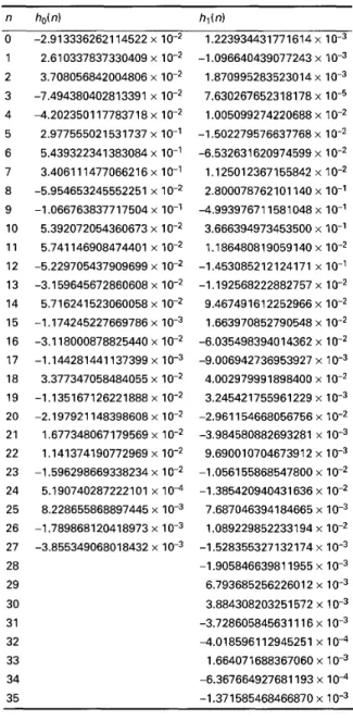
and q are set to 0.3, and respectively. The design process converges after 95 iterations, and we obtain the filter coefficients listed in Table 3 for the designed Ho(z) and H , ( z ) . Table 4 lists the PPRs and PSRs obtained using the proposed technique and the technique proposed by [12] for comparison. Again, we observe that the proposed design technique outper- forms the design technique of [12].

Table 3: Coefficients of designed analysis filters for example 2 n 0 1 2 3 4 5 6 7 8 9 10 - hdn) -6.725424402131615 x IO" -8.093401 185895091 x 4.284830277708982 x 3.934581458571292 x IO-' -7,433748861 139335 x 1 O-' -2.600001 179509680 x IO-' 2.777304396607232 x IO-' 5.375675495818721 x IO-' 3.520342050544742 x IO-' -4.204893884612326 x IO-' -1.3'14552401075692 x IO-' hJn) 2.546955245030047 x IO" 3.065015583801856 x -5.86076971 1466920 x IO4 -2.425850420051810 x 3.183001889098627 x IO-' 7.293957050668703 x IO-' -1.575952731003075 x IO-' -2.794869300505558 x IO-' 5.192844728914954 x IO-' -3.539047922494386 x IO-' -2.235498908352128 x IO-' 1 1 4.609381673833978 x IO-' 1.346173815175778 x IO-' 12 13 14 15 16 17 18 19 20 21 22 23 24 7.82956612201 1240 x -4.535170770214778 x IO-' -5.061291502985965 x IO-' 4.267834783769486 x IO-' 3.147848878057249 x IO-' -3.751001943708513 x IO-' -1.777678058856440 x IO-' 3.266046982329915 x IO-' 3.829358645729260 x -1.983184525933409 x IO-' -1.490288245827230 x 1 0-3 1.352347493301952 x IO-' -7.094584778960839 x IO" 2.302668873104872 x IO-' -8.318680180271586 x IO-' -2.060465751714644 x IO-' 5.657237541 164185 x IO-' 1.77693069997 1551 x 1 0-' -3.722270552852502 x -1.366323244651354 x IO-' 2.336349499957799 x IO-' 8.376281095944816 x -1.496726223860888 x IO-' -5.737426058036154 x IO" 6.145026937724032 x 1 0-3 -8.537891396719580 x IO" 25 -7.694762162301822 x -5.130128576649550 x 26 1.277493209581 154 x 1.696329957289639 x 27 3.309406212501463 x 4.068589144379184 x 28 -5.951942864417530 x IO" -6.476615778101027 x IO" 29 -2.164678025702934 x -2.7942481 11642598 x 30 9.689838062608440 x I 0-5 6.03822774671 2434 x I 0-5 31 5.060229848966466 x IO" 3.153284922368712 x IO"

The corresponding magnitude responses of Ho(z) and

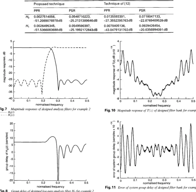
H l ( z ) are depicted in Fig. 7, and the corresponding group delays of Ifo(:) and H l ( z ) are depicted in Figs. 8 and 9, respectively. Moreover, the magnitude response and delay characteristic of T(z) are shown in Figs. 10 and 1 1, respectively.

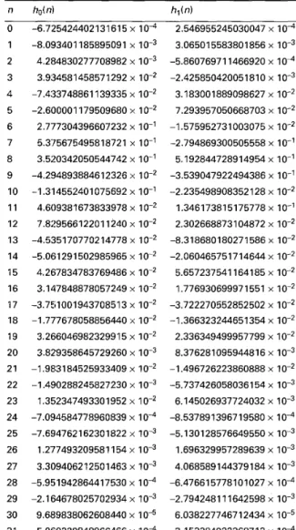
Table 4: Significant design results for example 2

Proposed technique Technique of [I21

PPR PSR PPR PSR Ho 0.0027514056, 0.05487 10223, 0.0135593391, 0.07 18047 133, HI 0.0026495345, 0.0549590397, 0.00704051 36, 0.0929426454, -51.2089076978dB -25.2131389646dB -37,355229576348 -22.8769409539dB -51.5366083688 dB -25.1992 172843dB -43.0479 131702 dB -20.6356994091 dB 0 0.1 0.2 0.3 0.4 0.5 normalised frequency

Magnitude responses of designed analysis filters for example 2

Fig.7 __ ff&) HI(^) - _ _ ~ 2o 15

c

normalised frequency

Fig. 8 Group delay of designed lowpass analysisfilter H, for example 2

0 0.1 0.2 0.3 0.4 0.5

normalised frequency

Fig.9 Group delay of designed high-pass analysisfilter H , for Example 2

6 Conclusions

This paper has presented a technique for the minimax design of low-delay two-channel perfect-reconstruction IEE Proc.-Vis. Image Signal Process., Vol. 144, No. 1, February 1999

2 0 -2 -4 -6 -8 0 0.1 0.2 0.3 0.4 0.5 normalised frequency

Fig. 10 Magnitude response of T ( z ) of designedfilter bunk for example 2

L

0.5

" - 8 1 I I ' ' I ' ' ' '

'

0 0.1 0.2 0.3 0.4

normalised frequency

Fig. 11 Error of system group delay of de.signedfilter bank for example 2

FIR filter banks. The design problem was first formu- lated as a nonlinear optimisation problem. The eigen- structure of the coefficient matrix for the constraints of perfect reconstruction was utilised to partition the filter coefficient vector into two components, namely the first component in the null space of the coefficient matrix and the second component orthogonal to this null space.

To alleviate the difficulty of nonlinear constraints, an approximation scheme has been proposed to linearise the nonlinear constraints for the filter frequency responses. Then, a technique based on the use of a modified dual-affine scaling variant of Karmarkar's algorithm was developed for updating the first compo- nent of the filter coefficient vector.

For perfect reconstruction, an approximation scheme has been proposed for updating the second component of the filter coefficient vector to guarantee the perfect- reconstruction characteristic of the designed filter banks. Moreover, analytical formulas have been pre- sented for choosing the appropriate desired responses of the analysis filters and calculating the step size

required at each iteration. As a result, the coefficients of the analysis filters can be obtained efficiently by solving only linear equations during the design process. Computer simulations have shown the effectiveness of the proposed design technique.

7 Acknowledgment

This work was supported by the National Science Council under grant NSC87-22 13-E002-071.

8 References

1 ESTEBAN, D., and GALAND, C.: ‘Applications of quadrature mirror filters to split band voice coding schemes’. Proceedings of IEEE international conference on Acoust., speech, signal process- ing, Hartford, Connecticut, 1977, May 1977, pp. 191-195 WOODS, J.W., and O’NEIL, S.D.: ‘Subband coding of images’,

IEEE Trans. Acoust. Speech Signul Process., Oct. 1986, ASSP-34, 3 GHARAVI, H., and TABATABAI, A.: ‘Sub-band coding of monochrome and color images’, IEEE Trans. Circuits Syst., Feb.

1988, CAS-35, pp. 207-214

KOILPILLAI, R.D., NGUYEN, T.Q., and VAIDYANATHAN, P.P.: ‘Some results in the theory of crosstalk free transmultiplex- ers’, IEEE Truns. Signul Process., Oct. 1991, 39, pp. 21742183

5 DOGANATA, Z., VAIDYANATHAN, P.P., and NGUYEN,

T.Q.: ‘General synthesis procedure for FIR lossless transfer matrices for perfect reconstruction multirate filter bank applica- tions’, IEEE Trans. Acoust. Speech Signal Process., Oct. 1988, 2

pp. 1278-1 288

4

ASSP-36, pp. 1561-1574

6 NGUYEN, T.Q., and VAIDYANATHAN, P.P.: ‘Two-channel perfect reconstruction FIR QMF structures which yield linear- phase analysis and synthesis filters’, IEEE Truns. Acoust. Speech Signal Process., May 1989, ASSP-37, pp. 676-690

7 VAIDYANATHAN, P.P., and HOANG, P.-Q.: ‘Lattice struc- ture for optimal design and robust implementation of two-chan- ne1 perfect-reconstruction Q M F banks’, ZEEE Trans. Acoust. Speech Signul P r o c e x , Jan. 1988, ASSP-36, pp. 81-94

VETTERLI, M., and LE GALL, D.: ‘Perfect reconstruction FIR filter banks: some properties and factorizations’, IEEE Truns. Acoust. Speech Signal Process., July 1989, ASSP-31, pp. 1057- 1071

9 SMITH, M.J.T., and BARNWELL, T.P.: ‘Exact reconstruction techniques for tree structured subband coders’, IEEE Trans. Acoust. Speech Signd Process., June 1986. ASSP-34, pp. 4 3 4 44 1

10 VETTEIRLI, M., and HERLEY, C . : ‘Wavelets and filter banks:

relationship and new results’. Proceedings of IEEE international 8

conferenceon Acoust. .speech signul procekirig, Albuquerque, New Mexico, Apr. 1990, pp. 1723-1726

11 NAYEBI. K.. BARNWELL. T.P.. and SMITH. M.J.T.: ‘Low delay FIR filter banks: design and evaluation’. IEEE Truns. Sig-

nu1 Process.. Jan. 1994, 42, pp. 2 4 3 1

12 ABDEL-RAHEEM, E., EL-GUIBALY, F., and ANTONIOU,

A.: ‘Design of low-delay two-channel FIR filter banks using con- strained optimisation’, Signul Process., 1996, 48, pp. 183-192 13 SCHEUERMANN, H., and GOCKLER, H.: ‘A comprehensive

survey of digital transmultiplexing methods’, Proc. IEEE, Nov. 1981, 69, pp. 1419-1450

14 ADLER, I., KARMARKAR, N., . RESENDE, M.G.C., and VEIGA, G.: ‘An implementation of Karmarkar’s algorithm for linear programming’, Math. Progrum.. 1989. 44, pp. 297-335 15 HILLIER, F.S., and LIEBERMAN, G.J.: ‘Introduction to math-

ematical programming’ (New York. McGraw-Hill, 1991) 16 TUNCER, T.E., and NGUYEN, T.Q.: ‘General analysis of two-

band Q M F banks’, IEEE Truns. Signul Process., Feb. 1995, 43, pp. 54&548