Adaptive phase field simulation of non-isothermal free dendritic growth of a binary alloy

www.actamat-journals.com

Adaptive phase field simulation of non-isothermal free

dendritic growth of a binary alloy

C.W. Lan

_{, Y.C. Chang}

_{, C.J. Shih}

a_{Department of Chemical Engineering, National Taiwan University, Taipei 10617, Taiwan, ROC} b_{Institute of Advanced Material Study, Kyushu University, 6-1 Kasuga Koen, Kasuga 816-8580, Japan}

Received 27 August 2002; received in revised form 27 November 2002; accepted 27 November 2002

Abstract

Efficient adaptive phase field simulation is carried out for a free dendritic growth in a nickel/copper system. The adaptive nature of the present scheme allows the simulation to be performed in an extremely large domain for thermal boundary layer, while keeping fine mesh for the diffusive interface. For isothermal cases, our calculated results agree reasonably well with those of Warren and Boettinger [Acta. Metall. Mater. 43 (1995) 689]. For non-isothermal growth, our results also agree well with those by Loginova et al. [Acta. Mater. Mater. 49 (2001) 573] for using a small domain. However, the domain size used in the previous calculations was too small for heat conduction, so that the calculated results are domain dependent and the dendrite could not grow freely. By choosing an extremely large domain, we have obtained a truly free growth simulation for the first time for a non-isothermal dendrite. The effect of supercooling is also illustrated and discussed.

2003 Acta Materialia Inc. Published by Elsevier Science Ltd. All rights reserved.

Keywords: Adaptive mesh refinement; Phase field simulation; Dendritic growth; Binary alloy; Tip speed PACS: 68.70.+w; 81.30.Fb

1. Introduction

The development of microstructures or dendrites is important in solidification processing or materials science [1]. However, the interplay of complex processes, including heat and mass trans-fer as well as interfacial and kinetic phenomena, imposes a formidable free-boundary problem being a great challenge to numerical simulation. Over the

∗ _{Corresponding author. Fax:+886-2-2363-3917.}

E-mail address: cwlan@ntu.edu.tw (C.W. Lan).

1359-6454/03/$30.002003 Acta Materialia Inc. Published by Elsevier Science Ltd. All rights reserved. doi:10.1016/S1359-6454(02)00582-7

past ten years or so, the phase field method has been used extensively for the simulation of den-dritic growth and the prediction of microstructures, e.g. [1–3]. Although the progress in the phase field simulation is significant, a quantitative prediction is still, in general, not available. Beside the model itself, the problem involves multi-length scales for the interface thickness and thermal and solutal boundary layers, and the difference is up to several orders. In addition, the physical time scales also differ significantly. Therefore, a major challenge ahead for a quantitative prediction of the micro-structure is in computation. In this report, we take

a non-isothermal Cu/Ni system as an example to report our new simulation results for a free den-dritic growth using an adaptive scheme. This adaptive phase field simulation uses an extremely large domain, so that the far field boundary con-ditions are not affected during the growth. There-fore, the calculated results could be useful as benchmarks for other simulations as well as ana-lytical predictions.

The simulation of non-isothermal free dendritic growth is not a trivial task in computation, especially for a metallic alloy, because thermal and solutal diffusions proceed in very different time scales. As the morphology evolves, the length scales by both processes also differ dramatically. Therefore, in the past most of the simulations tended to ignore the thermal diffusion by either using isothermal, e.g. [4], or frozen-temperature approximation [5]. Loginova et al. [6] made the first attempt to simulate the thermal and solutal transports simultaneously in a dendritic growth using an adaptive finite element method. Unfortu-nately, they only illustrated the differences by incorporating the energy calculations and showed that the latent heat does affect significantly the simulated morphologies and temperature. For benchmark comparison, such a simulation is inad-equate because the results are domain dependent, and the boundary effect is significant as well. In other words, their dendrite did not grow freely, but was constrained in a small box with a constant wall temperature or cooling rate.

In this report, we re-examine the same problem by using an extremely large domain, so that a “free” growth and its structure development can be obtained under given supersaturation and super-cooling. The domain chosen here is large enough for a thermal boundary layer which is about four orders in magnitude larger than the solutal one. Meanwhile, the numerical mesh is fine enough for the interface and solutal fields. As such, the domain independent solution can be obtained. Some useful information including the dendrite tip speed, maximum domain temperature, and the effects of noises and supercooling, as well as the solute trap-ping, are also presented. In the next section, the phase field model and the adaptive finite volume method are described briefly. Section 3 is devoted

to results and discussion, followed by conclusions and comments in Section 4.

2. Adaptive phase field simulation

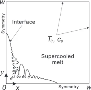
The dendritic growth from a small circle seed in a large supercooled Ni/Cu melt at composition c0

and temperature T0, as shown in Fig. 1 for a quarter

of the full domain, is simulated here. Because the crystallographic directions have been aligned with the coordinate axes, a quarter domain is adequate for simulation. For comparison purposes, the model employed in [4] and [6] is also adopted here. This model at constant temperature was first pro-posed by Wheeler, Boettinger and McFadden [7], the so-called WBM model, using the minimization of a Gibbs free energy function. Penrose and Fife [8] and Warren and Boettinger [4] further derived a similar model based on an entropy function, which can be used in non-isothermal growth. How-ever, the temperature effect was ignored in the pre-vious simulation until recently. Loginova et al. [6] took the energy Eq into account, where some ideas due to Caginalp and Xie [9] were introduced. In fact, adding the energy Eq does not increase the

Fig. 1. A schematic of a binary dendrite growing freely in a supercooled and supersaturated melt.

computation time much. The problem is that the heat conduction for the metallic system is much faster than solute diffusion. To simulate the prob-lem in a realistic manner having a given tempera-ture at the far field requires an extremely large domain, which makes the calculation difficult with-out using an adaptive mesh. In order to present the governing Eqs in dimensionless form, the variables are rescaled. The temperature is rescaled to q=(T⫺Tref)/⌬T, where Trefand⌬T are the reference

temperature and temperature difference, respect-ively. The concentration (atomic fraction) c is rescaled by c0 to c∗, where c0 is the far field

con-centration. The length, in terms of the coordinates

x and y, is rescaled by l and time t by l2_/D L to

t∗, where l is a characteristic length and l2_/D Lis a

characteristic time; DL is the solute diffusivity in

the liquid. The phase filed variable f is set to be 1 in liquid and 0 in solid, while 0.5 at the interface. Then, the governing Eqs used in [6] can be rep-resented in dimensionless form:

C˜∗∂q ∂t∗⫹

冉

冊

冋

冉

冊

冉

冊册

where C˜∗is the normalized heat capacity being scaled by the value at c0, i.e. C˜∗ = C˜ / C˜(c0). The

variable with a tilde is the concentration-weighted average. For example, the heat capacity C˜ is defined by

C˜ ⫽ (1⫺c)CA⫹ cCB, (4)

where CAand CBare the heat capacity of the sol-vent (A) and the solute (B). Inside the diffusive interface, the properties are weighted by a function

p(f) from a double-well function g(f), which is

defined by g(f) =f2₍₁⫺f)2_{. The weighting}

func-tion p(f) for the averaged physical properties of the solid/liquid mixture is chosen such that

p’(f)=30g(f). For example, the normalized diffu-sivity of the solution is given by:

D∗⫽ D/D(c0)⫽ [Ds⫹ p(f)(DL⫺DS)] / DL, (5)

where the individual diffusivity has been assumed not affected by the solute concentration, e.g.

D(c0)=DL; both DS and DL are assumed constant

here, i.e. D ⬅ D˜. The Stefan number S˜t ⬅

C˜ (c0)⌬T/⌬H˜, where ⌬H˜ is the heat of fusion,

while the Lewis number L˜e ⬅ a˜/DL, where a˜ ⬅

K˜ / C˜(c0) is the concentration-averaged thermal

diffusivity. In addition, S∗A and S∗B are the nor-malized entropy of A and B, respectively, being scaled by R/Vm, i.e. S∗i = SiVm/ R, (i=A or B); Vm

is the molar volume and R the gas constant. The entropies of A and B are defined as the following:

SA(f,T)⫽ WAg⬘(f) ⫹ p⬘(f)⌬HA

冉

冊

冉

冊

where WAand WBare constants and TAmand TBmare

the melting points of A and B, respectively; ⌬HA and⌬HBare the heats of fusion per volume. Again, in Eq (3), S˜∗is the concentration-averaged value, i.e. S˜∗= (1⫺c)S∗A+ cS∗B.

The anisotropic functionh in Eq (3) is defined for the four-fold symmetry as:

h⫽ 1 ⫹ gcos4b, (8)

where g is the intensity of the anisotropy and b

= tan⫺1[(∂f /∂y) / (∂f /∂x)] determining the growth

orientation of the dendrite. In this study, we have purposely chosen (100) in the x-direction and (010) in the y-direction, so that the four-fold symmetry allows us to take a quarter domain for simulation, which saves computational effort significantly. Finally, the dimensionless mobility function M˜∗f being scaled by DLVm/(Rl2) is taken from the

aver-age of Mi = Ti2mbi/ (6√2⌬Hidi), i=A or B, where bi is the kinetic coefficient anddithe interface

thick-ness, which are assumed to be the same for A and

B here. Similarly, e˜∗2_{is a dimensionless parameter} being rescaled by l2_{. For each component, e}2

i = 6√2sidi/ Tim, wheresiis the interfacial energy. All

the parameters chosen are the same as those in [6], which are similar to the ones used in the WBM model [7].

method has been used. The detailed implemen-tation of the scheme can be found elsewhere [9,10]. In order to have a constant setting of the far field boundary conditions, i.e. c=c0 and T=T0, the

domain needs to be large enough for a truly free growth. As such, the simulations can be inde-pendent of the domain size and meaningful for benchmarking with theories. Therefore, the simul-ation starts at a small circular seed (radius r0=2l) in

a large domain, which corresponds to 2D uniform lattices having 214×₂14×₂₀×_{20 cells here; the}

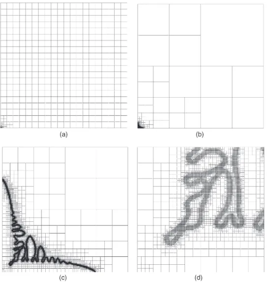
small-est cell size is 0.61l at the 15th level and largsmall-est cell size (⌬x) 10,000l at the first level (20×20). At the symmetric boundaries, no-flux condition is imposed. At the far field boundaries, the dimen-sionless concentration is set to unity, while the dimensionless temperature is⫺1. A sample mesh during growth is shown in Fig. 2, where we have viewed the mesh at four different length scales. As shown, mesh refinement is performed by subdivid-ing uniformly each parent cell into four kid cells. As such, detailed substructures can also be described nicely if the mesh level is large enough; in Fig. 2, W=200,000l and 15 levels of grid are used having the smallest cell size 0.610l and the largest 10,000l. Two criteria are used for the refinement. One is based on the phase field variable (refinement for 0.05⬍f⬍0.95) and one for the con-centration (refinement for 0.1⬍ |ⵜc|). In addition, the level difference for adjacent cells is also restric-ted to one, so that the mesh size increases gradually from the finest region and this improves signifi-cantly the accuracy of the method. By mapping the grid into a quad-tree data structure, the dynamic pointer functions in FORTRAN90 can be fully adopted and this makes the programming straight-forward. The implicit Euler scheme is used for time integration and this allows larger integration times-teps to be used. Nevertheless, the limitation for the timesteps is that the interface advancement needs to be inside the refined zone. Otherwise, numerical instability can cause problems. Accordingly, for the smaller interface thickness d, if the total num-ber of cells is kept the same, the timestep needs to be reduced as well. This also increases compu-tation time. In the present simulation, the CPU time for a growth scales about W2 _{for a given interface} thickness. In other words, the computational cost

is about linearly proportional to the domain area. This is comparable to the performance of the scheme proposed by Provatas et al. [11].

3. Results and discussion

For comparison purposes, the Ni/Cu system used by Warren and Boettinger [4] and Loginova et al. [6] is considered here. The physical properties and system related parameters, unless otherwise stated, are the same as those in [6]; ⌬T=20.5 K,

Tref=1594.5 K, T0=1574 K, c0=0.4083,g=0.04, and

timestep⌬t∗=0.2, etc., as well as those phase field parameters. The interface thickness (d=4.9×10⫺8 m) is chosen to be the same as the one used by Loginova et al. [6], though there is about 30% dif-ference in the steady tip speed as compared with that at d=2.2×10⫺9 m. The isothermal calculation is much easier because the diffusion boundary layer is very thin and one could choose a small domain for calculation. In such a case, the solutal boundary layer builds up quickly and a steady den-drite tip speed can be reached after t∗⬎50 (or 0.108 ms). Accordingly, the small domain size W=750l is enough, where l=0.94d is chosen. On the other hand, for non-isothermal calculations, due to the fast thermal diffusion, a significant larger domain is necessary. Several domain sizes have been chosen, and we have picked up the largest one (W=200,000l) for illustration. For comparison, we also introduce artificial noises [4,6] by

∂f ∂t∗→ ∂f ∂t∗⫺M˜ ∗ far(16g(f))S˜∗, (9) where a is the noise intensity and r the random number ranging from ⫺1 to 1. Our calculated result for the isothermal growth with the noises of

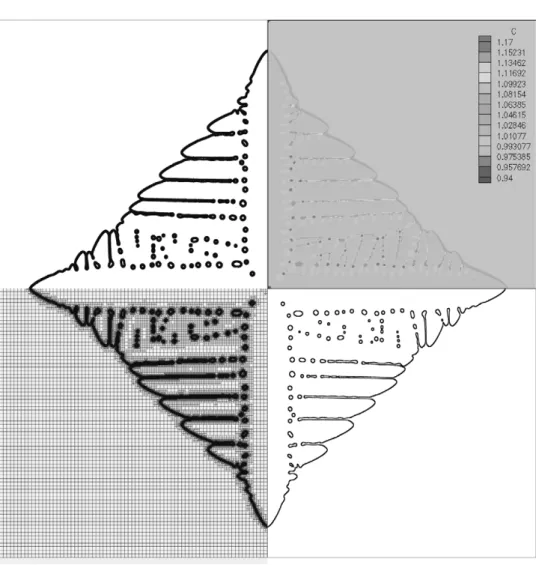
a=0.4 at t∗=1000 (or 2.17 ms) is shown in Fig. 3; only 5 levels of grid are used due to the small domain (W=750l). The largest cell size (⌬x) at the first level of the grid (75×75) is 10l and the small-est cell size is 0.625l at the fifth level of the grid. As shown, the mesh adapts to the dendrite structure nicely, while a very thin boundary layer is in front of the dendrite. Due to the small solutal boundary layer, a small domain is adequate for calculation as long as the solute boundary is not too close to

Fig. 2. A sample adaptive mesh in different viewing windows: (a) 200,000l×200,000l; (b) 10,000l×10,000l; (c) 625l×625l; (d) 156.25l×156.25l; the largest cell size is 10,000l and the smallest one is 0.610l.

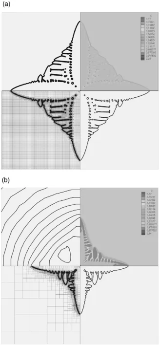
the boundary. A smaller cell size can be chosen, but the result is not affected much. In fact, our smallest cell size here is already smaller than the one used by Warren and Boettinger [4] and Logi-nova et al. [6]. Although the microstructure and the steady-state tip speed (1.3 cm/s) agree reasonably well with that (~1 cm/s) by Warren and Boettinger [4], the development of our dendrite in the grove part is slightly faster. It is particularly true for no artificial noises (a=0). Without noises, as shown in Fig. 4(a), we also have a significant structure development at t∗=1000. In other words, it is

pre-sumed that the numerical noises due to the adaptive grid seem to be larger than those by uniform mesh used in the previous reports, so that the dendrite tends to develop faster as compared with that in [4]. Indeed, the substructure is sensitive to the noises. Thus, the stochastic nature of the morpho-logical development makes the further quantitative comparison difficult. In reality, the thermal noises are hard to control as well. Therefore, getting an identical microstructure for the same condition, even in experiments, is also difficult as well.

Fig. 3. Calculated solutal fields (upper right), phase fields (upper left), mesh (lower left), and the interface (lower right) for isothermal growth at T0=1574 K with artificial noises at a=0.4; domain size W=750l, while the smallest cell size is 0.625l (the fifth level) and

the largest one is 10l (the first level).

having the temperature fixed at the far field bound-ary, and the result at t∗=1000 is shown in Fig. 4(b); we keep the noise intensity the same at a=0.4. However, the domain considered is much larger (W=200,000l), even though we only show a small potion of it in Fig. 4(b). As shown, for the same growth time, as compared with Fig. 3, the non-isothermal growth is significantly slower and the developed side branches are much less. No clear solute trapping is found as well; in Figs. 3 and 4(a), one could see many trapped melt packets inside the dendrite. Apparently, this is due to the release of latent heat, which produces a thermal barrier to

reduce supersaturation (supercooling). The tem-perature increases near the growth front leading to less driving force for the growth. The development of side branches is also slower. In the shown win-dow, 705l×750l in Fig. 4(b), the temperature is not constant along the window boundary indicating that the heat diffuses way beyond the small win-dow. Accordingly, for a free growth a much larger domain is necessary. This is the main reason why we need such a large domain (W=200,000l) for cal-culation.

This can be better understood from the time evolution of concentration and thermal fields, as

Fig. 4. (a) Isothermal growth at a=0; (b) non-isothermal growth at a=0.4; the upper left of (b) is the thermal field; the computation domain for (b) is 200,000l×200,000l.

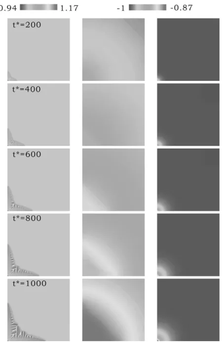
shown in Fig. 5. The results in the first two col-umns are the solutal and thermal fields, respect-ively, viewed from a small window (750l×750l), while the third column is for thermal fields viewed from a much larger window (20,000l×20,000l). As shown, although the solutal boundary layer is thin (the first column), the thermal one (the second and the third columns) is much thicker due to the much larger thermal diffusivity in the metallic system. The thermal diffusivity a˜ being 2.7×10⫺5 m2_{/s is}

much larger than the solute diffusivity (10⫺9m2_/s).

One can see that at t∗=1000, the heat has diffused widely beyond the smaller window. Even with the large window in the third column, the spreading area is quite significant being about half of the win-dow.

Estimating the domain size required for free dendrite growth is straightforward. The thermal boundary layer thicknessdTcan then be estimated bya˜ / Vs, which is about 45,500l; Vsis the dendrite

tip speed (~0.85 cm/s). This estimation is quite reasonable, which can also be judged easily later in Fig. 11. Similarly, the solutal boundary thick-ness (dc) is only about 1.7l, which is four orders smaller than dT. Although the solutal boundary layer from this estimation is not much larger than the smallest grid size (0.610l here), the use of a smaller grid size does not affect the solution much. This is simply due to the fact that the actual solute varies over several δc (~5×1.7l). Therefore, the smallest size used here, which is still smaller than the ones used in [4 and 6], is adequate. As just mentioned, for the isothermal case, the steady tip speed can be reached before t∗=50. Therefore, for a realistic simulation of a free growth in a metallic system, which should not have the boundary effect, the domain needs to be much larger than the ther-mal boundary layer. By doing several calculations using different domain sizes, we found that 4~5dT is adequate. The domain we have used for calcu-lation has a width of 200,000l. The whole domain size related to the dendrite size can be seen from Fig. 2(a).

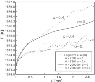
The time evolution of the maximum temperature in the domain is shown in Fig. 6; we have pur-posely used dimensional temperature and time for illustration here. The results with different domain sizes and noises are put together for comparison.

Fig. 5. Time evolution of solutal (first column) and thermal (second and third columns) fields for non-isothermal growth at T0=1574

K and a=0.4; the first two columns are viewed from a small window at 750l×750l, while the third column is viewed from a larger window of 20,000l×20,000l.

Indeed, with the thermal noises, due to the faster development of the size branches in the 45° direc-tion (the groove), the maximum temperature is higher than that of no noises (a=0) due to the more latent heat being released. Because the maximum

temperature is not at a fixed point, but moves around depending on the structure development, the curves are less smooth especially with noises. When a branch is growing, the latent heat is released so that the temperature increases.

How-Fig. 6. Time evolution of the maximum temperature in the domain during growth for different domain sizes and noises.

ever, when two branches merge and stop growing, the temperature also stops increasing and the maximum temperature will appear elsewhere hav-ing the faster growth. The temperature oscillation is thus an indication of the branching activity. For the smaller domain, due to the faster growth rate, and more side branching, the oscillation is much more significant than that in a large domain. The calculated result by Loginova et al. [6] is also put together for comparison; they used W=750l and

a=0.4 for calculation. As shown, the agreement is quite satisfactory. With the larger domain (W=200,000l), the temperature increase is signifi-cantly larger than that of the smaller domain; the thermal oscillation is less and no oscillation is observed for the case without noises indicating much less branching. On the contrary, in the smaller domain, the boundary temperature is fixed at a constant temperature, so that the growth is for-ced to cool down faster when the thermal boundary layer is getting close.

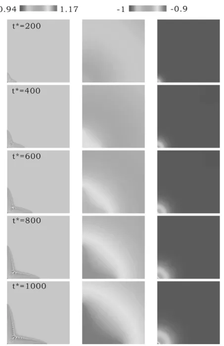
Fig. 7 shows the similar time evolution of the solutal and thermal field for the same condition, but without the noises (a=0). As shown, the devel-opment of side branches is significantly delayed. Because of the much less branching, the maximum temperature in the domain increases smoothly, as we just mentioned in Fig. 6. We have also put the

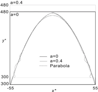
overall tip shapes of the previous two calculations at t∗=1000 for comparison, and the parabolic fitting is also included in Fig. 8. Although the non-iso-thermal growth is driven by concentration differ-ence, and suppressed slightly by the temperature barrier due to the heat of fusion, the overall den-drite shape can still be described by a parabola nicely, except near the tip, where the interfacial effect is significant due to the small radius of cur-vature. Adding noises will not affect the tip mor-phology much, but enhances the side branching. Also, as just mentioned for Fig. 6, the warming effect from the faster growth of side branches, with noises, the tip growth rate is also lower. In Fig. 8, we have purposely shifted the result in the y-direc-tion for comparison.

The tip speeds for different domain sizes are illustrated in Fig. 9. The one with noises in a large domain is also included for comparison. In all cases, the growth is getting slower and slower, and does not reach a steady state, except the one in the smallest domain size (W=750l). Due to the forced cooling at the boundary, reducing the domain size increases the growth rate. As a result, for the small-est domain size (W=750l), the tip speed increases when the tip is impinging on the boundary. When the domain is large enough, we have obtained the time evolution of tip speed that is not affected by the domain size. Nevertheless, due to the very dif-fused thermal field, the warming effect from the side arms could reduce the tip speed, so that a ste-ady tip speed is also not possible. The very slow settling of the tip speed was also observed by Pro-vatas et al. [11] at low supercoolings. In their cal-culations, the near-steady tip speed is somewhat different from the solvability limit because of the side arm effect. With noises, the growth rate fluc-tuates much more significantly. Of course, the growth rate is slightly lower than the one without noises. Again, this is because of the faster develop-ment of side branches producing more heat (also see Fig. 6) that slows down the tip growth. One should notice that the fluctuation of the tip speed exists even without the noise. This is simply due to the interpolation error in the speed estimation from f=0 [12,13]. The morphologies at t∗=1300 for the largest domain size at a=0 and a=0.4 are also illustrated in the same figure for reference.

Fig. 7. Time evolution of solutal (first column) and thermal (second and third columns) field for the nonisothermal growth at T0=1574

K and a=0; the first two columns are viewed from a small window at 750l×750l, while the third column is viewed from a larger window of 20,000l×20,000l.

In the previous calculations, we have kept the melt at 1574 K in the far field for the comparison with the isothermal result [4], and the release of latent heat significantly reduces the growth. It is also clear that one can also put the seed in a

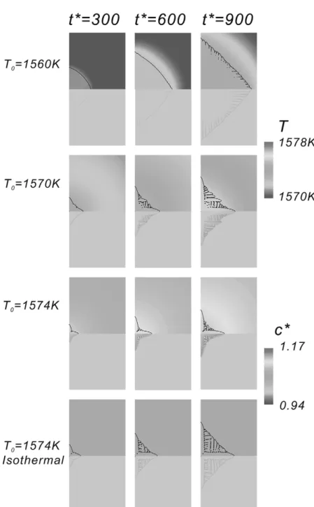
super-cooled melt, and a much faster development of the dendrite can be anticipated. To do so, we have also tried several lower ambient temperatures (a=0.4), and the results are summarized in Fig. 10; we also put the results of previous two calculations

Fig. 8. Dendrite tip shapes from Figs. 5 and 7 at t∗=1000; the parabolic fittings are also included for comparison; the vertical scale for a=0.4 (slower growth) is shifted upward for compari-son.

Fig. 9. Time evolution of tip growth speed at different domain sizes. For the largest domain size, the one with artificial noises (the lowest curve) is included for comparison; the attached den-drite shapes are obtained from the largest domain.

(T0=1574 K) for comparison. As shown, when the

melt is colder, the growth is faster, but the develop-ment of the detailed structure is delayed. In a sig-nificantly cooled melt (T0=1560 K), the overall

shape exhibits a circular shape, with some fine morphological development at the later time. One can also observe the solute buildup in front of the interface becomes much less at high supercooling. This is believed to be the more significant solute trapping due to the finite interface thickness [14– 16]. At t∗=900, at the interface, Cs/CL=0.956

(measured from primary arm along the x-direction) for T0=1560 K, as compared with 0.939 at 1570 K

and 0.929 at 1574 K. For the isothermal situation,

Cs/CL=0.944 due to the larger growth rate. Similar

results were also observed in previous calculations [6] by controlling the cooling rate in a small domain. The velocity-dependent segregation was also discussed by Aziz [14] and Aziz and Kaplan [15] and it is related to the interface diffusion speed. Based on the derivation of Ahmad et al. [16], the interface diffusion speed is about 0.484 cm/s, and our growth rates in all cases are larger than this value. This indicates that solute trapping may occur in all cases, but the case in the coolest melt is the most severe one. Furthermore, since the solute trapping is due to the diffusive interface, an accurate interface thickness is necessary to describe the phenomena quantitatively. However, as mentioned at the beginning, the smaller interface requires a smaller timestep and thus longer com-puting time, and for a realistic interface thickness, the computing effort required could be at least one or two orders more.

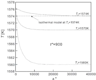
At t∗=900, the thermal profiles in front of the primary arm in the x-direction are plotted in Fig. 11 for different supercoolings. As shown, there is a significant warming effect in front of the growing tip. In a cooler melt, the tip temperature (at xi=0) is also lower indicating a larger supercooling (having a larger tip curvature) at the tip, which drives the growth faster to consume the supercool-ing. The cooling rates estimated from Fig. 11, based on VdT/dx|max, are about 843, 2188, 5550 K/s

for T0=1574, 1570, and 1560 K, respectively.

Although these values are much smaller than those specified in [6], which was estimated at the initial stage, the observed phenomena are similar, and one

Fig. 10. Time evolution of the growth at different supercooled melts. In each supercooled temperature, the upper figures are the isotherms and the interface shape (solid line) and lower are the solutal fields.

may take the lowest domain temperature in [6] as

T0in the present calculations to find the similarity.

However, in the previous calculations, the way of specifying the cooling rate is quite artificial and

difficult to be related to a doable growth experi-ment in practice.

Fig. 11. Temperature distribution in front of the primary side arm (in the x-direction) for different supercoolings at t∗=900.

4. Conclusions and comments

We have presented an efficient adaptive phase simulation for non-isothermal free dendritic growth of a binary alloy. The simulation uses a large enough domain size for thermal diffusion, with small enough cells for the diffusive interface and solutal gradients. Our smallest cell size is smaller than the previous ones, while the domain size is several orders larger. Reasonably good agreement with previous studies is obtained for using a small domain. As the domain increases, the heat accumu-lation in front of the interface is significantly higher and the growth speed lower, as compared with those obtained from a much smaller domain size. As a result of the slower growth, solute trap-ping is significantly reduced. The artificial noises also significantly affect the results due to the enhanced growth of side branches. The warming effect due to the very diffused thermal field in the metallic system significantly lowers the tip speed and inhibits a steady tip growth, even in a large domain. In addition to supersaturation, thermal driven growth is also illustrated by using different supercooled melts. In the colder melt, the faster growth induces more solute trapping and thus reduces solutal gradients. This makes the growth

more thermally driven. Although the use of the adaptive scheme is efficient, there are still some limitations here, such as the thick interface thick-ness and the small kinetic coefficient used. Fortu-nately, they could be resolved by using a more powerful computer and longer CPU time. Simul-ation including convection is underway and the effect of microflow, which is much faster than the diffusion, can also be investigated in the near future.

Acknowledgements

CWL would like to thank Professor N. Imaishi for his generous hospitality for the CWL’s three-month stay in Kyushu University. The visiting Pro-fessorship to CWL sponsored by Kyushu Univer-sity is highly appreciated. We are grateful for the valuable comments from the referees. This research is sponsored by the National Science Council of the Republic of China.

References

[1] Wheeler AA, Ahmad NA, Boettinger WJ, Braun RJ, Mac-Fadden GB, Murray BT. Adv. Space Res. 1995;16:163. [2] Boettinger WJ, Coriell SR, Greer AL, Karma A, Kurz W,

Rappaz M, Trivedi R. Acta Mater 2000;48:43.

[3] Ode M, Kim SG, Suzuki T. ISIJ International 1076;2001:41.

[4] Warren JA, Boettinger WJ. Acta metal. 1995;43:689. [5] Boettinger WJ, Warren JA. Metall. Mater. Trans

1996;27A:657.

[6] Loginova I, Amberg G, Argen J. Acta mater. 2001;49:573. [7] Wheeler AA, Boettinger WJ, McFadden GB. Phys. Rev.

A 1995;45:7424.

[8] Penrose O, Fife PC. Physica D 1990;43:44.

[9] Lan CW, Hsu CM, Chang YC. Phys. Rev. E 2002;65:61601.

[10] Lan CW, Liu CC, Hsu CM. J. Comp. Phys. 2002;178:464. [11] Provatas N, Goldenfield N, Dantzig J. Phys. Rev. Lett.

1988;80:3308.

[12] Karma A, Rappel WJ. Phys. Rev. E 1995;53:3017. [13] Jeong J-H, Goldenfeld N, Dantzig JA. Phys. Rev. E

2001;64:041602.

[14] Aziz MJ. J. Appl. Phys 1982;53:1158.

[15] Aziz MJ, Kaplan T. Acta. Metall. 1988;36:2335. [16] Almad NA, Wheeler AA, Boettinger WJ, McFadden GB.