An Efficient Approach to Discovering Repeated Sequential Patterns in Large Transaction Databases

全文

(1)(1) Workshop: Workshop on Databases and Software Engineering (2) Title: An Efficient Approach to Discovering Repeated Sequential Patterns in Large Transaction Databases (3) Abstract: Data mining, also known as knowledge discovery, is recognized as an area of promising research. It can be defined as the efficient discovery of interesting patterns from a large database. Mining sequential patterns involves discovering patterns in sequences of events with a user-defined minimum support. The support of a pattern is the number of data-sequences that include the pattern. The previous approach, the GSP（generalized sequential patterns）algorithm, checks whether a data-sequence contains a specific sequence for counting candidates requiring alternates between the forward and backward phases until all the items are found. The higher complexity of operations is performed repeatedly to detect certain particular items. In this paper, a DRSP algorithm using two additional Order list and Check list data structures is proposed, to reduce the complexity of sequence search. The proposed approach can also discover the repeated sequential pattern, which include several overlapped items. Experimental results indicate that the proposed searching approach outperforms GSP algorithm. (4) Author: (A) Chien-I Lee,. Addr: Institute of Information Education, National Tainan Teachers College Tainan, Taiwan 700, R.O.C. E-mail: [email protected] Tel: (886)6-2133111 ext. 777 Fax: (886)6-2144409 (B) Meng-Sung Wu,. Addr: Department of Computer Science and Information Engineering, National Cheng Kung University, Tainan, Taiwan, R.O.C E-mail: :[email protected] TEL:06-2089349 (5) Name of the contact author:. Chien-I Lee. (6) Keyword: Data mining, Sequential Patterns. 1.

(2) An Efficient Approach to Discovering Repeated Sequential Patterns in Large Transaction Databases. Chien-I Lee1, Meng-Sung Wu2 1. Institute of Computer Science and Information Education,. National Taiwan Teachers College, Tainan, Taiwan, R.O.C. E-mail:[email protected] 2. Department of Computer Science and Information Engineering, National Cheng Kung University, Tainan, Taiwan, R.O.C. E-mail:[email protected]. Abstract. Data mining, also known as knowledge discovery, is recognized as an area of promising research. It can be defined as the efficient discovery of interesting patterns from a large database. Mining sequential patterns involves discovering patterns in sequences of events with a user-defined minimum support. The support of a pattern is the number of data-sequences that include the pattern. The previous approach, the GSP（generalized sequential patterns）algorithm, checks whether a data-sequence contains a specific sequence for counting candidates requiring alternates between the forward and backward phases until all the items are found. The higher complexity of operations is performed repeatedly to detect certain particular items. In this paper, a DRSP algorithm using two additional Order list and Check list data structures is proposed, to reduce the complexity of sequence search. The proposed approach can also discover the repeated sequential pattern, which include several overlapped items. Experimental results indicate that the proposed searching approach outperforms GSP algorithm.. 2.

(3) 1 Introduction Data mining can be defined as the process of discovering hidden and potentially useful information in an extremely large database. As an important part of market analysis and an important use of the Internet, data mining is used in many applications in which interesting rules can be extracted from large collections of data. Discovering sequential patterns from a large database of sequence is an area of active researches into data mining. The purpose of mining sequential patterns is the detection of all sequences whose support exceeds the user-defined minimum support. A sequential patterns is represented as <s1s2…sn>, where sj is an itemset. An itemset (a set of items) is denoted as <i1i2…im>, where ij is an item. The support counts for a sequence defined as the fraction of all data-sequences that ‘include’ this sequence. An example of such a sequential pattern is that customers bought ‘Camera’, then ‘Camera and Negative’, and then ‘Digital Camera and Memory Card’. Most researchers focus not only on improving the effectiveness of data mining but also developing various algorithms to determine various kinds of sequential patterns for mining. Previous research [1, 2, 3, 4, 5, 6, 7, 8, 9, 10, 11, 12, 13] has almost attached importance to execute efficiency and a relation of sequence. Many techniques have been proposed for mining sequence patterns. The GSP algorithm [2] have considered the time gap between adjacent items of the sequences, however, when a sequence is too long, it is inefficient to do several switching between forward and backward processes until all the items are found in searching a specific sequence. On the other hand, the DSG (Direct Sequential pattern Generation) algorithm [11], which uses the graph architecture to find sequence patterns, needs to scan the database only once. Although the algorithm reduces the cost of accessing I/O, it increases the cost of accessing the main memory. As the database expands, it may not be fit in the memory. Accordingly, Zaki [13] proposed the SPADE (Sequential Pattern Discovery using Equivalence classes) algorithm to solve the problem. This algorithm used a lattice-theoretic and simple intersection method 3.

(4) that decomposed the original search space into smaller pieces that can be fit in the memory. However, these main-memory algorithms are unsuitable when the potential sequence patterns are so large that the graph architecture cannot be fit in the memory. Jiawei Han et al. [5] presented the FP-tree method, which also involves scanning the database only once. The method does not need to generate which candidates, and the supports can be obtained from the constructed FP-tree. Even so, it is the same problem with DSG, which a large amount of memory space needs is taken by the constructed FP-tree. Therefore, in this paper, we propose an efficient searching heuristic algorithm to discover sequential patterns, the DRSP (Discovery Repeated Sequential Patterns) algorithm, which is modified from the GSP algorithm and considered with time constraints to remedy the performance bottleneck in searching a specific sequence using check-table structures. The repeated sequential pattern is a group of several overlapped items in the sequential pattern. An example of such a pattern is that customers bought ‘Camera’, then ‘Negative’, and then ‘Digital Camera’, and then ‘Negative’. Thus, it can be seen that the ‘Negative’ is an overlapped item in the sequence. The experimental results show that newly proposed searching approach outperforms the GSP algorithm The rest of the paper is organized as follows. Section 2 describes the problem of mining generalized sequential patterns. Section 3, we present the proposed searching heuristic approach to discover frequent occurring sequential patterns. In Section 4, we evaluate the performance of the proposed approach. Conclusions and areas for future research are finally made in Section 5.. 4.

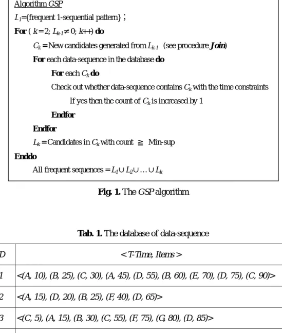
(5) 2 Mining Generalized Sequential Patterns Mining sequential patterns involve finding sequence of transaction data. All of a customer’s transactions can be viewed as a sequence, the list of transactions, and orders by increasing transaction-time corresponding to a sequence. At the same time, the customer doesn’t have the same transactions. The GSP algorithm [2] as shown in Fig. 1 has to scan the database in multiple passes. Throughout mining, many candidate sequences must be counted to determine the frequently occurring sequences. The sliding window relaxes the restriction so the items in the sequential pattern don’t have to come from the same transaction. The time constrains can avoid a time period too far or too close between the adjacent items in a pattern. Thus, there are two parameters, max-gap, and min-gap, are proposed to deal with these time constraints. The max-gap denotes that the time gap between sets of item no more than maximum time gap constraint, and the min-gap denotes that the time gap between adjacent sets of item no less than minimum time gap constraint. For illustration purpose, we use the simple example shown in Tab. 1 is used to explain the process of the GSP algorithm. Each record is a {SID, < T-Time, Items >} pair, where SID is the identifier of the corresponding sequence, T-Time is the transaction time of purchasing, and Items is the element in the sequence. The minimum support, Min-sup, represents the minimum number of a sequence has to appear in order to be qualified as a frequently sequence. In this example, Min-sup is set to 2. After the database of data-sequence in Tab. 1 is scanned, the frequently 1-sequential pattern is found in the database as shown in Tab. 2. Then, in the for-loop process, the frequent occurring sequences LK-1 (k≧2) from the previous pass are used to generate the candidate sequences CK and then their support is counted. The support of the candidates is used to determine whether they are the frequent sequences (such that the support ≧ Min-sup). This for-loop process is repeated until no candidate sequence is generated or no more frequent sequence is found.. 5.

(6) Algorithm GSP L1={frequent 1-sequential pattern}； For ( k = 2; Lk-1≠0; k++) do Ck = New candidates generated from Lk-1 (see procedure Join) For each data-sequence in the database do For each Ck do Check out whether data-sequence contains Ck with the time constraints If yes then the count of Ck is increased by 1 Endfor Endfor Lk = Candidates in Ck with count ≧ Min-sup Enddo All frequent sequences = L1∪L2∪…∪Lk. Fig. 1. The GSP algorithm. Tab. 1. The database of data-sequence SID. < T-Time, Items >. S1. <(A, 10), (B, 25), (C, 30), (A, 45), (D, 55), (B, 60), (E, 70), (D, 75), (C, 90)>. S2. <(A, 15), (D, 20), (B, 25), (F, 40), (D, 65)>. S3. <(C, 5), (A, 15), (B, 30), (C, 55), (F, 75), (G, 80), (D, 85)>. S4. <(B, 15), (A, 25), (D, 40), (C, 65)>. Tab. 2. The supports of frequent 1-sequence Frequent 1-sequence. Support. A. 4. B. 4. C. 3. D. 4. F. 2. 6.

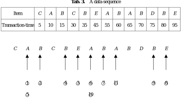
(7) During a pass, the GSP algorithms read one data-sequence at a time and increase the support count of candidates contained in the data-sequence. Thus, given a set of candidates sequence and a data-sequence, all sequences in the candidate sequences contained in a data-sequence must be found. The GSP algorithm alternates between the forward phases and backward phases to check whether a data-sequence contains a specific sequence,. The algorithm starts in the forward phase from the first element. An example illustrates the process. Suppose the dataset, DS = <A, B, C, D, E, F, G> includes seven items and consider a user’s data-sequence as shown in Tab. 3. Consider the case when max-gap is 20 time units, and min-gap and the size of the sliding-windows are zero. For the candidate sequence <A, B, E>, first find “A” at transaction-time 10, then find “B” at transaction-time 15. Since the max-gap constraint between “A” and “B” is satisfied, it continues to move forward. Then, find “E” at transaction-time 45, since the gap between “B” and “E” (30days) exceeds max-gap, and discards “B”. Then, moves backward. Because end-time (“E”) = 45 and max-gap is 20, then searches for the first appearance of “B” after transaction-time 25. Found “B” at transaction-time 35. Check whether the max-gap constraint between “B” and the previous item “A” is satisfied, because “B” is not the first item. The max-gap constraint between “B” and “A” is more than max-gap (i.e., time (“B”) - time (“A”) = 35 –10 = 25), so it moves forward, to search for the first occurrence of “A” at time 55. Because “A” is the first element, we do not need check whether the max-gap constraint is satisfied. Then continues to move forward and found “B” at transaction-time 60. Repeated this procedure, until all the items are found. Finally, found the sequence <A, B, E> for which the corresponding transaction-time is (65, 80, 95). Throughout the procedure, the GSP algorithm takes 11 comparisons to find the sequence <A, B, E>, as shown in Fig. 2. When a data-sequence is long in mining sequential pattern process. Checking out whether a data-sequence contains a specific sequence using the GSP algorithm is inefficient. The following section proposes an efficient approach, called the DRSP algorithm, to solve this problem. 7.

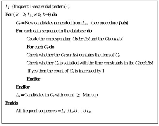
(8) Tab. 3. A data-sequence Item. C. A. B. C. B. E. A. B. A. B. D. B. E. Transaction-time 5. 10. 15. 30. 35. 45. 55. 60. 65. 70. 75. 80. 95. B. D. B. E. 9 ○. 8 ○. C. A. B. ○ 1. 2 ○. C. B. E. A. B. A. 4 ○. 3 ○. 6 ○. 7 ○. 11 ○. 10 ○. 5 ○. Fig. 2. Using the GSP algorithm to search sequence pattern <A, B, E>. 3 The DRSP Approach This section propose the DRSP algorithm as shown in Fig. 3, which is modified from the GSP algorithm to search whether a data-sequence includes a specified candidate sequence. Additionally, the process of discovering repeated sequential patterns. During a pass, searching for the candidate sequences contained in a data-sequence involves checking whether a data-sequence contains a specific sequence and the counting of it. The GSP algorithm [2], is repeated, switching between the backward and forward phases until all the items are found. However, when a data-sequence is long, it is inefficient. Therefore, an approach is improved to improve this problem using two additional data structures, called the Order list and the Check list, respectively. Let P = < p1, …pm > be the set of the all items in the transaction database. For a candidate sequence s = < s1, …sn > with N items, there creates a 1 x N array Op of the Order list. Each cell is corresponding to an item in alphabetical order. Let the value of Op(si) = i, 1 ≤ i ≤ n and the value of the other Op(j) = -1, where j ∉ s. For the candidate sequence s = < s1, …sn >, there creates a n x n array Cs of the Check list, where the initial values of all cells are –1. 8.

(9) L1={frequent 1-sequential pattern}； For ( k = 2; Lk-1≠0; k++) do Ck = New candidates generated from Lk-1 (see procedure Join) For each data-sequence in the database do Create the corresponding Order list and the Check list For each Ck do Check whether the Order list contains the item of Ck Check whether Ck is satisfied with the time constraints in the Check list If yes then the count of Ck is increased by 1 Endfor Endfor Lk = Candidates in Ck with count ≧ Min-sup Enddo All frequent sequences = L1∪L2∪…∪Lk. Fig. 3. The DRSP algorithm The proposed efficient approach to checking out a specific sequence is summarized as follows: For the data-sequence, check whether an Order list contains the item of data-sequence. If the item exists, check the difference between the time of the item just found and the previous item. If the difference satisfies the gap constrains, then store the values of time that correspond to the position of the Check list, and then reproduced the values of all the previous specified items. Repeat this process until all the items of a specific sequence are found and the time constraint is always satisfied. That is, when the value of Cs(n, n) is changed from –1 to the T-time of the last item sn in the data-sequence, the answer of the sub-sequence in the data-sequence that contains the candidate-sequence s = < s1, …sn > will be < Cs(n, 1), Cs(n, 2),…Cs(n, n)>. On the other hand, no answer is found when Cs(n, n) is still –1 after the last item of the data-sequence is scanned. Tab. 4. The Order list for the candidate sequence <A, B, E> si. A. B. C. D. E. F. G. Op(si). 1. 2. -1. -1. 3. -1. -1. 9.

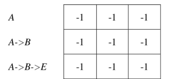
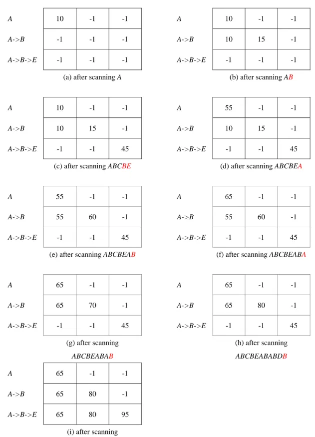
(10) Tab. 5. The initial Check list for the candidate sequence <A, B, E> A. -1. -1. -1. A->B. -1. -1. -1. A->B->E. -1. -1. -1. The same example as shown in Tab. 3 is considered here, The max-gap = 20 time units, and min-gap = sliding-windows size = zero. For the candidate sequence <A, B, E>, we generate the Order list with N = 7 items as shown in Tab. 4, and an initial 3 x 3 array of Check list as shown in Tab. 5 are generated. For the data-sequence as shown in Tab. 4, if at first item “A” is scanned at transaction-time 10 and position 1 in the Order list, then the values of the time that correspond to the position of the Check list can be stored, as shown in Fig. 4-(a) (i.e., Cs (1, 1) = 10). Then item “B” can be scanned at transaction-time 15 and position 2 in the Order list (i.e., Cs (2, 2) = 15). The value of Cs (2, 1) is set to the value of Cs (1, 1) since the max-gap constraint between “A” and “B” is satisfied (i.e., 15 - 10 < 20),. Then, item “C” is scanned; and can be discarded since it is absent from the Order list (i.e., Ps (C) = -1). For the next scanned item “B” at transaction-time 35, because the gap between “B” and “A” (25days) is more than the max-gap, and so is discarded after “B”. Item “E” continues to be scanned at transaction-time 45, and then the values of time that correspond to the position of the Check list are stored, as shown in Fig. 4-(c) (that is, Cs (3, 3) = 45). Next, item “A” is scanned at transaction-time 55, and the record of pre-item “A” that corresponds to the position of the Check list is overwritten, as shown in Fig. 4-(d) (that is, Cs (1, 1) is updated to “55”). Similarly, after item “B” is scanned, Cs (2, 2) is set to 60 and the value of Cs (2, 1) is set to the value of Cs (1, 1) as shown in Fig. 4-(e). The candidate sequence <A, B, E> can be found by analogy. Then, the checking process is stopped and the count of <A, B, E> is increased by one for all the items of the candidate sequence <A, B, E> which are involved in the final row of the Check List whose values still satisfying the time constraint. The proposed heuristic is used to search sequence <A, B, E>, using nine comparisons, as shown in Fig. 4. 10.

(11) A. 10. -1. -1. A. 10. -1. -1. A->B. -1. -1. -1. A->B. 10. 15. -1. A->B->E. -1. -1. -1. A->B->E. -1. -1. -1. (a) after scanning A. (b) after scanning AB. A. 10. -1. -1. A. 55. -1. -1. A->B. 10. 15. -1. A->B. 10. 15. -1. A->B->E. -1. -1. 45. A->B->E. -1. -1. 45. (c) after scanning ABCBE. (d) after scanning ABCBEA. A. 55. -1. -1. A. 65. -1. -1. A->B. 55. 60. -1. A->B. 55. 60. -1. A->B->E. -1. -1. 45. A->B->E. -1. -1. 45. (e) after scanning ABCBEAB. (f) after scanning ABCBEABA. A. 65. -1. -1. A. 65. -1. -1. A->B. 65. 70. -1. A->B. 65. 80. -1. A->B->E. -1. -1. 45. A->B->E. -1. -1. 45. (g) after scanning. (h) after scanning. ABCBEABAB. ABCBEABABDB. A. 65. -1. -1. A->B. 65. 80. -1. A->B->E. 65. 80. 95. (i) after scanning ABCBEABABDBE. Fig. 4. The values of the Check list Cs during the process of checking out a specific sequence. 11.

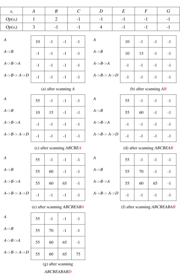
(12) Tab. 6. The Order list for the candidate sequence <A, B, A, D> si. A. B. C. D. E. F. G. Op(si). 1. 2. -1. -1. -1. -1. -1. Op(si). 3. -1. -1. 4. -1. -1. -1. A. 10. -1. -1. -1. A. 10. -1. -1. -1. A->B. -1. -1. -1. -1. A->B. 10. 15. -1. -1. A->B->A. -1. -1. -1. -1. A->B->A. -1. -1. -1. -1. A->B-> A->D. -1. -1. -1. -1. A->B-> A->D. -1. -1. -1. -1. (a) after scanning A. (b) after scanning AB. A. 55. -1. -1. -1. A. 55. -1. -1. -1. A->B. 10. 15. -1. -1. A->B. 55. 60. -1. -1. A->B->A. -1. -1. -1. -1. A->B->A. -1. -1. -1. -1. A->B-> A->D. -1. -1. -1. -1. A->B-> A->D. -1. -1. -1. -1. (c) after scanning ABCBEA. (d) after scanning ABCBEAB. A. 55. -1. -1. -1. A. 55. -1. -1. -1. A->B. 55. 60. -1. -1. A->B. 55. 70. -1. -1. A->B->A. 55. 60. 65. -1. A->B->A. 55. 60. 65. -1. A->B-> A->D. -1. -1. -1. -1. A->B-> A->D. -1. -1. -1. -1. (e) after scanning ABCBEABA A. 55. -1. -1. -1. A->B. 55. 70. -1. -1. A->B->A. 55. 60. 65. -1. A->B-> A->D. 55. 60. 65. 75. (f) after scanning ABCBEABAB. (g) after scanning ABCBEABABD. Fig. 5. The values of the Check list Cs during the process of checking out a specific sequence 12.

(13) However, when the sequential patterns include several overlapped items, as in the sequence <A, B, A, D>, the GSP algorithm cannot find it. Therefore, based on the proposed heuristic approach, the M x N array Order list must be generated, where M is the number of the overlapped items. As in the above example, for the candidate sequence <A, B, A, D>, we create a 2 x 7 array Op of the Order list, as shown in Tab. 6, and an initial 4 x 4 array of Check list are created. If item “A” is first scanned, then the values of time that correspond to the position of the Check list can be stored, as shown in Fig. 5-(a) (that is, Cs (1, 1) = 10). Then item “B” can be scanned at transaction-time 15 and position 2 in the Order list (that is, Cs (2, 2) = 15). The value of Cs (2, 1) is set to the value of Cs (1, 1) since the max-gap constraint between “A” and “B” is satisfied (that is, 15 - 10 < 20). Then, item “C” is scanned; can be discarded since it is absent from the Order list (that is, Ps (C) = -1). The above approach implement, until all the items are found. On the other hand, when searching the second “A” at transaction-time 55, is the need to check end-position 3 in the Order list. Because the gap between “B” and “A” (40days) exceeds max-gap, the values of time that correspond to position 1 of the Check list can be stored, as shown in Fig. 5-(c) (that is, Cs (1, 1) = 55). Next, item “B” is scanned at transaction-time 60, and the record of pre-item “B” that correspond to the position of the Check list is overwritten, as shown in Fig. 5-(d) (that is, Cs (2, 2) is updated to “60”). Similarly, after item “A” is scanned, Cs (3, 3) is set to 65, and the value of Cs (3, 1) and Cs (3, 2) are set to the value of Cs (2, 1) and Cs (2, 2) respectively, as shown in Fig. 5-(e). To continue, item “B” is searched and only the record of pre-item “B” is overwritten, as shown in Fig. 5-(f). Finally, the candidate sequence <A, B, A, D> can be found using the proposed heuristic to searching sequence <A, B, A, D>, using seven comparisons, as shown in Fig. 5.. 13.

(14) 4 Performance Study In this section, compare the performance of our DRSP algorithm with the GSP algorithm. We refer to [1] to generate the synthetic database. The synthetic data generation program takes the parameters as shown in Tab. 7. The number of data-sequences was set to D = 250,000. We generated datasets by setting Ns = 5000, Ni = 25000 and N = 10000. Tab. 8 shows the datasets with their parameter settings. Tab. 7. Parameters |D|. Number of customers (= size of Database). |C|. Average number of transaction per customer. |T|. Average number of items per transaction. |S|. Average length of maximal potentially frequent sequences. |I|. Average size of Itemsets in maximal potentially frequent sequences. Ns. Number of maximal potentially frequent sequence. Ni. Number of maximal potentially large itemsets. N. Number of items. Tab. 8. Parameter settings (Synthetic datasets) Name. |C|. |T|. |S|. |I|. Size(MB). C10-T2.5-S4-I1.25. 10. 2.5. 4. 1.25. 23.8. C10-T5-S4-I1.25. 10. 5. 4. 1.25. 25.1. C10-T5-S8-I2.5. 10. 5. 8. 2.5. 26.2. C20-T2.5-S4-I1.25. 20. 2.5. 4. 1.25. 36.1. C20-T2.5-S8-I2.5. 20. 2.5. 8. 2.5. 36.5. On the synthetic databases, each graph shows the results as the minimum support changes from 1% to 0.2%. Assume the sliding-window’s size is zero, without minimum and 14.

(15) maximum gap constrains. Fig. 6 shows the relative execution times for the DRSP, AprioriAll and GSP algorithms, on C10-T2.5-S4-I1.25 synthetic dataset given in Tab. 8. From Fig. 6, we observe that the GSP algorithm is faster than the DRSP algorithm. The reasons is that GSP algorithm doesn’t have to check whether a data-sequence contains a specific sequence, but our approach still needs time to create the Order list and Check list. Hence, without time constrains, the GSP algorithm is outperforming the DRSP algorithm. Certainly, the GSP algorithm is better than the AprioriAll algorithm as proved in [2]. To see the effect of the sliding windows and time constrains in performance, we tested the DRSP algorithm and the GSP algorithm on the four datasets. The sliding window was set to zero. Similarly, the max gap was set to more than the total time-span of the transactions in the datasets and the min gap was set to 2 time units. Fig. 7 shows that the DRSP algorithm outperforms the GSP algorithm. The main reason is that the numbers of specific candidate sequence counting for the DRSP algorithm are fewer than the GSP algorithm. The GSP algorithm has to check whether a data-sequence contains a specific sequence by switching the forward and backward phases alternately. Thus the number of scanned items increases.. C 10 - T 2.5-S4 - I 1.25 16 GSP. 14. AprioriAll. Time(min). 12. DRSP. 10 8 6 4 2 0 1. 0.5. 0.33. 0.25. 0.2. Min - Sup(%). Fig. 6. Performance Comparison: (without time constrain). 15.

(16) C 10 - T 5 -S8- I 2.5. C 10 - T 5-S4 - I 1.25 50. 50 GSP. GSP. 40. DRSP. 30. Time(min). Time(min). 40. 20. DRSP. 30. 20 10. 10. 0. 0 1. 0.5. 0.33. 0.25. 1. 0.2. 0.5. C 20 - T 2.5-S4 - I 1.25. 0.25. 0.2. C 20 - T2.5 -S8- I 2.5. 50. 50. GSP 40. GSP 40. DRSP. 30. Time(min). Time(min). 0.33 Min - Sup (%). Min - Sup (%). 20. 10. DRSP. 30. 20. 10. 0 1. 0.5. 0.33. 0.25. 0. 0.2. 1. Min - Sup (%). 0.5. 0.33. 0.25. 0.2. Min - Sup (%). Fig. 7. Performance Comparison: (with time constrains). 5 Conclusions In this paper, proposed and studied efficient method for mining frequent repeated sequential patterns in large sequence database. The DRSP algorithm, which is modified from the GSP algorithm, to search whether a data-sequence contains a specified candidate sequence by using two additional data structures, called the Order list and the Check list. From the experimental study, we compared our DRSP algorithm with the GSP algorithm, and the result shows that our algorithm outperforms the GSP algorithm. The main reason is that the GSP algorithm has to do several switching between forward and backward processes until the 16.

(17) entire items are found in searching a specific sequence. On the other hand, the DRSP algorithm scans all the items in the data-sequence at one time. We have been studying how to further improve the performance at discovering repeated sequential patterns, how to mine efficiently cyclic-sequential patterns, and how to incorporate user-specified constraints at mining such patterns. The application of sequential pattern mining in Weblog analysis and DNA analysis are also interesting topics for future research.. References 1. R.Agrawal, R.Srikant. Mining Sequence Patterns. Proceedings of the 11th International Conference on Data Engineering (1995) 3-10. 2. R. Agrawal, R. Srikant. Mining Sequential Patterns: Generalizations and Performance Improvements. Proceeding of the Fifth Int'l Conference on Extending Database Technology (EDBT) (1996) 3-17. 3. Y. Bengio. Probabilistic neural network models for sequential data. IJCNN (2000). 4. M.-S. Chen, J.-S. Park, & P. S. Yu. Efficient Data Mining for Path Traversal Patterns. IEEE Transactions on Knowledge and Data Engineering (1998) 209-221, 10(2). 5. J. Han, J. Pei, & Y. Yin. Mining frequent patterns without candidate generation. Proceedings of the ACM SIGMOD on Management of data (2000).. 6. N. G. Minos, R. Rajeev, S. Kyuseok. Sequential Pattern Mining with Regular Expression Constraints. Proceedings of 25th International Conference on Very Large Data Bases (1999) 7. B. Mobasher, N. Jain, E.-H. Han., J. Srivastava. Web Mining: Pattern Discovery from World Wide Web Transactions. Department of Computer Science University of Minnesota Minneapolis (1996). 8. M. Oglhara. Scalable feature mining for sequential data. IEEE Intelligent Systems [see also 17.

(18) IEEE Expert] (2000) Volume: 15 48-56 9. J. Pei, J. Han, B. Mortazavi-Asl, H. Pinto, Q. Chen, U. Dayal, and M.-C. Hsu. PrefixSpan: Mining sequential patterns efficiently by prefix-projected pattern growth. In ICDE (2001). 10. F. Qin, X.-B. Yang. A high efficient algorithm of mining sequential patterns. Proceedings of the 3rd World Congress on Intelligent Control and Automation (2000) 11. S.-J. Yen, Arbee L.P. Chen. An Efficient Approach to Discovering Knowledge from Large Database, PDIS (1996) 8-18. 12. S.-J. Yen. Mining Frequent Traversal Patterns in a Web Environment. In Proceeding of International Symposium on Intelligent Data Engineering and Learning (1998) 219-224. 13. M. J. Zaki. Efficient Enumeration of Frequent Sequences. CIKM (1998) 68-75.. 18.

(19)