A High-Speed Feature Selection Method For Large Dimensional Data Set

全文

(1)A High-Speed Feature Selection Method For Large Dimensional Data Set Wei-Chou Chen, Ming-Chun Yang, Shian-Shyong Tseng*. Department of Computer and Information Science National Chiao Tung University Hsinchu 300, Taiwan, R. O. C. E-mail: sstseng@cis.nctu.edu.tw. Abstract Feature selection is about finding useful (relevant) features to describe an application domain. The problem of finding the minimal subsets of Features that can describe all of the concepts in the given data set is NP-hard. In the past, we had proposed an feature selection method, that originated from rough set and bitmap indexing techniques, to select the optimal (minimal) feature set for the given data set efficiently. Although our method is sufficient to guarantee a solution’s optimality, the computation cost is very high when the number of features is huge. In this paper, we propose the nearly optimal feature selection method, called bitmap-based feature selection method with discernibility matrix, which employs a discernibility matrix to record the important features during the construction of the cleansing tree to reduce the processing time. And the corresponding indexing and selecting algorithms for such feature selection method are also proposed. Finally, some experiments and comparisons are given and the result shows the efficiency and accuracy of our proposed method. Keywords: bitmap feature selection method, performance, feature selection, bitmap indexing, rough set.. *Corresponding Author. 1.

(2) 1. Introduction. Feature selection is about finding useful (relevant) features to describe an application domain. Generally speaking, the function of feature selection is divided into three parts: (1) simplifying data description, (2) reducing the task of data collection, and (3) improving the quality of problem solving. The benefits of having a simple representation are abundant such as easier understanding of problems, and better and faster decision-making. In the case of data collection, having less features means that less data should be collected. As we know, collecting data is never an easy job in many applications because it could be time-consuming and costly. Regarding the quality of problem solving, the more complex the problem is if it has more features to be processed. It can be improved by filtering out the irrelevant features that may confuse the original problem, and it will win the better performance. There are many discussions about feature selection, and many existing methods to assist it, such as bit-wise indexing[2][3][4], GA technology [1][12], entropy measure[7][6], and rough set theory[19][12]. In the past, we had proposed an efficient feature selection method, that originated from rough set and bitmap indexing techniques, to select the optimal (minimal) feature set for the given data set. Although our method is sufficient to guarantee a solution’s optimality, the computation cost is very high when the number of features is huge. In this paper, we propose the nearly optimal feature selection method, called bitmap-based feature selection method with discernibility matrix, which employs a discernibility matrix to record the important features during the construction of the cleansing tree to reduce the processing time. And the corresponding indexing and selecting algorithms for such feature selection method are also proposed. Finally, some experiments and comparisons are given and the result shows the efficiency and 2.

(3) accuracy of our proposed method. This paper is organized as follows. The reviews of the relative work are given in Section 2. The bitmap-based feature selection method with discernibility matrix and its corresponding definitions and algorithms are proposed in Section 3. In Section 4, some experiments and discussions are made. At last, the conclusions are given in Section 5.. 2. Related Work Feature selection is about finding useful (relevant) features to describe an application domain. The problem of feature selection can formally be defined as selecting minimum features M’ from original M features where M’. Љ M such that the. class distribution of M’ features is as similar as possible to M features [8]. Generally speaking, the function of feature selection is divided into three parts: (1) simplifying data description, (2) reducing the task of data collection, and (3) improving the quality of problem solving. The benefits of having a simple representation are abundant such as easier understanding of problems, and better and faster decision-making. In the case of data collection, having less features means that less data should be collected. As we know, collecting data is never an easy job in many applications because it could be time-consuming and costly. Regarding the quality of problem solving, the more complex the problem is if it has more features to be processed. It can be improved by filtering out the irrelevant features that may confuse the original problem, and it will win the better performance. There are many discussions about feature selection, and many existing methods to assist it, such as bit-wise indexing[2][3][4], GA technology [1][12], entropy measure[7][6], and rough set theory[19][12]. The rough set theory, proposed by Pawlak in 1982 [7], can serve as a new. 3.

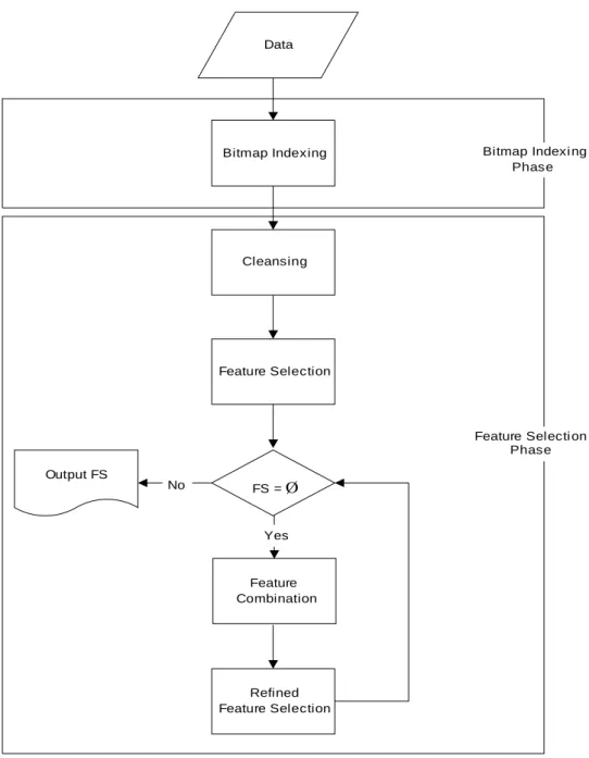
(4) mathematical tool for dealing with data classification problems. It adopts the concept of equivalence classes to partition training instances according to some criteria. Two kinds of partitions are formed in the mining process: lower approximations and upper approximations. Rough sets can also be used for feature reduction and the features that do not contribute towards the classification of the given training data will be removed. The problem of finding the minimal subsets of attributes that can describe all of the concepts in the given data set is NP-hard. Thus, researchers proposed several heuristic algorithms to reduce the computation time for such problem. In this paper, a new, efficient feature selection method originated from rough set is proposed. Moreover, the bitmap indexing techniques are also applied in this method for accelerating the feature selection procedure. The bitmap-based feature selection method is a feature selection method, that originated from rough set and bitmap indexing techniques, to select the optimal (minimal) feature set for the given data set efficiently. This method consists of Bitmap Indexing Phase and Feature Selection Phase. In the Bitmap Indexing Phase, the target table is first transformed into a bitmap indexing matrix with some further classification information. In the Feature Selection Phase, a feature-based spanning tree is first built for cleansing the bitmap indexing matrix and the cases with noisy information are thus filtered out. After that, a class-based table generated from the correct bitmap indexing matrix is built, and the bitwise operators "AND" and "OR" are thus applied to get optimal feature sets for decision making. The flowchart of the proposed method is shown in Figure 1.. 4.

(5) Data. Bitmap Indexing. Bitmap Indexi ng Phase. Cleansing. Feature Selection. Feature Selecti on Phase Output FS. No. FS = Ø. Yes. Feature Combination. Refined Feature Selection. Figure 1. Flowchart of bitmap-based feature selection method. 3. Bitmap-based feature selection method In Chapter 3, the bitmap-based feature selection method for feature selection is proposed to combine features to check if the new feature set is good enough to solve the problem. As we know, when the number of features is large, the optimal solution becomes impractical. Although an exhaustive search is sufficient to guarantee a. 5.

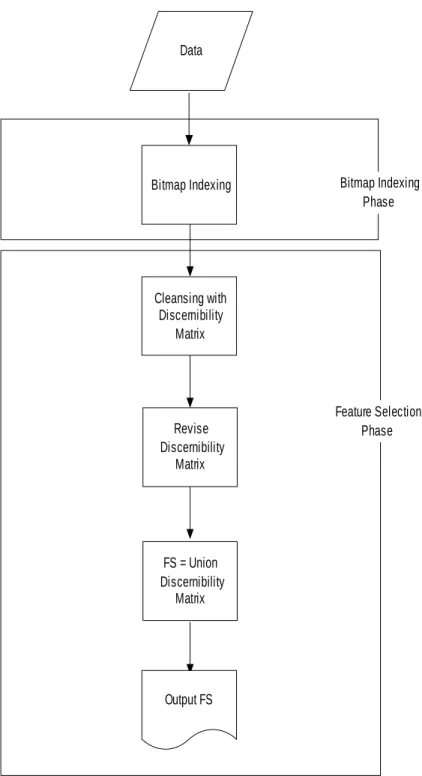
(6) solution’s optimality, the computation cost is very high in many real problems. Therefore, we propose the bitmap-based feature selection method with discernibility matrix which employs a discernibility matrix to record the important features during the construction of the cleansing tree to reduce the processing time. Based upon the cleansing tree, the discernibility matrix of bitmap-based feature selection is generated and the nearly optimal solution will be obtained. The flowchart of bitmap-based feature selection method with discernibility matrix is shown in Figure 2.. 6.

(7) Data. Bitmap Indexing. Bitmap Indexing Phase. Cleansing with Discernibility Matrix. Revise Discernibility Matrix. Feature Selection Phase. FS = Union Discernibility Matrix. Output FS. Figure 2. Flowchart of bitmap-based feature selection method with discernibility matrix. The definitions of proposed method are described in detail in the following sub-section. 3.1. Problem Definitions. 7.

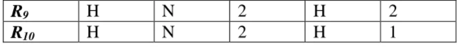
(8) Assume that there is a target table in a database, denoted as T. Set R is the set of records in T, denoted as R= {R1, R2, …, Rn} where n is the number of records in T. Assume C is the features domain of T, denoted as C={C1, C2, …, Cm} and m is the number of features in T. All features except Cm, a decision feature, are condition features. For each feature Cj of record Ri, its feature value is denoted as Vj(i) and Vj(i) ≠ null. Denote the feature value domain of Cj as Vj={Vj1, Vj2, …,Vj σ j }, where each element in Vj is a possible feature value of Cj and σj is the number of distinct values of Cj. In the next two sub-sections, the bitmap indexing phase and feature selection phase are described in detail with their corresponding definitions and algorithms.. 3.2 Bitmap Indexing Phase In this sub-section, the target table is first transformed into a bitmap indexing matrix with some further classification information. Initially, denote ONEk and ZEROk as the bit strings with length k, and all bits in the vector are set to 1 and 0 respectively. Denote UNIQUEk as a bit string with length k, and only one bit in the vector is set to 1 and the others are set to 0. In Figure 3, the target table T which shows a dataset containing ten records R={R1, R2, …, R10} and five features C={C1 ,C2 ,C3 ,C4} { C5}, where C5 is a decision feature and others are condition features.. R1 R2 R3 R4 R5 R6 R7 R8. C1 M M L L M L H H. C2 L L L R R R R N. C3 3 1 1 3 2 3 3 3 8. C4 M H M M M L L L. C5 1 1 1 2 2 3 3 3. Ж.

(9) R9 R10. H H. N N. 2 2. H H. 2 1. Figure 3. Target table T. Definition 1: Record vector The record vector Fjk.record is a bit string denoting the associated relationships of the k-th feature value of feature Cj in record set R, where 1 ≤ j ≤ m. Fjk.record = b1b2…bn. Set bi to 1 if Vj(i) equals to Vjk ; otherwise set bi to 0.. According to the definition of Record vector, the BelongToClass algorithm is proposed to get the corresponding Class vector by given record vector.. Algorithm 1: BelongToClass Input : Record vector Fjk.record Output : Class vector classjk Step 1:. Set classjk to ZEROσm.. Step 2:. For each i, where 1 ≤ i ≤ σm, set the i-th bit of classjk to 1 if the result of using "AND" bitwise operator on recordjk and Fmi.record is not equal to ZEROn; otherwise, set it to 0.. Step 3: Return classjk.. Definition 2: Class vector The class vector Fjk.class is a bit string denoting the class distribution of Fjk.record, where 1 ≤ j ≤ m and 1 ≤ k ≤ σj. Fjk.class = b1b2…b σm , σm is the number of distinct values of Cm. Class vector can be obtained via applying BelongToClass algorithm. 9.

(10) Definition 3: Feature-value vector The feature-value vector Fjk consists of record vector and class vector with the k-th feature value of the j-th feature, where 1 ≤ j ≤ m and 1 ≤ k ≤ σj.. Definition 4: A matrix of feature-value vectors  F j1    F j2  A matrix Mj of its feature-value vectors for feature Cj is denoted as   , where M    F jσ j . σj is the number of distinct values of Cj.. Applying bitwise operator "OR" on all record vectors of feature-value vector in Mj can get the ONEn vector, and applying bitwise operator "AND" on any two record vectors of feature-value vector in Mj can get the ZEROn vector. According to the above definitions and notations, it can be easily seen that Fj1.record OR Fj2.record OR…OR Fj σ j .record = ONEn, and Fja.record AND Fjb.record = ZEROn, where 1 ≤ a,b ≤ σj and a≠b. Obviously, Fj1.record XOR Fj2.record XOR …XOR Fj σ j .record = ZEROn.. Definition 5: A matrix of all features for a table T M 1  M  A matrix TM of all features for a table T is denoted as  2  , where m is the M    M m . number of the features. 10.

(11) Example 1: As shown in Figure 3, there are five features in the target table. According to Definitions 4 and 5, the matrix TM is shown in Figure 4.. Feature Feature-value Record M1. M2. M3. M4. M5. Class. F11. 1100100000 110. F12. 0011010000 111. F13. 0000001111 111. F21. 1110000000 100. F22. 0001111000 011. F23. 0000000111 111. F31. 1001011100 111. F32. 0110000000 100. F33. 0000100011 110. F41. 1011100000 110. F42. 0100000011 110. F43. 0000011100 001. F51. 1110000001 100. F52. 0001100010 010. F53. 0000011100 001. Figure 4. A matrix TM of five features for a table T. It’s necessary to keep the state of records for cleansing module in feature selection phase. If a record is processed via cleansing module and the result shows it should be further investigated, the record is valid; otherwise, the record is invalid.. Definition 6: Valid mask vector The valid mask vector ValidMask is a bit string denoting whether the records of 11.

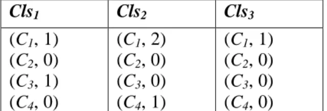
(12) R are valid or not. ValidMask =b1b2…bn. Set bi to 1 if Ri is valid; otherwise set bi to 0, where 1 ≤ i ≤ n. Initially, the ValidMask is set to ONEn.. As we can see, there are ten records in the target table T in Figure 3. The initial valid mask vector is ValidMask = b1b2…b10 = "1111111111" = ONEn.. 3.3 Feature Selection Phase The first step in Feature Selection Phase is a cleansing procedure. The difference in cleansing procedure between bitmap-based feature selection method and bitmap-based feature selection method with discernibility matrix is that the latter completes the feature selection after a cleansing tree is generated. Thus, the discernibility matrix is proposed to record the important features in cleansing module.. Unlike the original definitions of discernibility matrix in rough set which concerns the relationship between records and features [7], we redefine the class-based discernibility matrix to describe the relationship between classes and features. The main idea is that the original discernibility matrix saves information faithfully but may be time-consuming and space-waste, and feature-classes relation seems to more intuitional to problem-solving. Thus we propose the new definition of class-based discernibility matrix as below.. Definition 7: A class-based discernibility matrix. Cls1  Cls  2  A class-based discernibility matrix D is denoted as  , where Clsi is  M   Clsσ m  12.

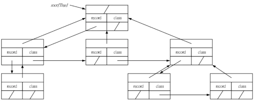
(13) composed by (Cj, weightij) and weightij is the summary of Cj used to determine class i where 1 ≤ i ≤ σm and 1 ≤ j ≤ m-1.. Example 2. If there are four condition features and three classes, the possible class-based discernibility matrix is shown in Figure 5. The weight11 and weight13 are 1 since the first class needs one C1 and one C3 to determine. Similarly, the weight21 is 2, the. weight24 and weight31 are 1.. Cls1. Cls2. Cls3. (C1, 1) (C2, 0) (C3, 1) (C4, 0). (C1, 2) (C2, 0) (C3, 0) (C4, 1). (C1, 1) (C2, 0) (C3, 0) (C4, 0). Figure 5. A possible class-based discernibility matrix. Before the feature selection phase is triggered, the correctness of the target table needs to be verified. In the target table, if there are some records with different decision feature values but the same values of all condition features, these records cannot be distinguished and thus are treated as noise. The first step of feature selection phase is to filter out the noisy records from the target table. The intuitional method to find out the inconsistent records in the target table is to compare every two different records, it may take O(n2m) times, where n is the number of records and m is the number of features. In order to reduce the time complexity of the above straight forward method, a cleansing tree is proposed to decrease the time complexity to O(nm). A cleansing tree Ctree is a rooted tree (with root root[Tree]). The maximum of height of the root[Tree] is m-1. Every node x has three pointers, including p[x], 13.

(14) left-child[x] and right-sibling[x], which point to parent, to the leftmost child and to the right sibling of x, respectively. Also, each node x contains some extra information; e.g.. record[x] and class[x] contained in node x indicate the associated record and class of x, respectively. If node x has no child, then left-child[x] = NIL; if node x is the rightmost child of its parent, then right-sibling[x] =. NIL.. A typical cleansing tree is shown in. Figure 6.. ̅̂̂̇ˮ˧̅˸˸˰. ̅˸˶̂̅˷. ˶˿˴̆̆. ̅˸˶̂̅˷. ˶˿˴̆̆. ̅˸˶̂̅˷. ˶˿˴̆̆. ̅˸˶̂̅˷. ˶˿˴̆̆. ̅˸˶̂̅˷. ̅˸˶̂̅˷. ˶˿˴̆̆. ˶˿˴̆̆. ̅˸˶̂̅˷. ˶˿˴̆̆. Figure 6. A cleansing tree structure. Definition 8: Spanned Feature Order The spanned feature order O is a sequence consists with the m-1 condition features {Cα1, Cα2,…,Cα(m-1)}, Cαi∈C-Cm, ∀Cαi and Cαj, Cαi≠Cαj, where 1 ≤ i ≤ m-1, 1 ≤ j ≤ m-1 and i ≠ j.. In the cleansing tree Ctree, all nodes in the level i of root[Tree] are associated with a unique condition feature Oi=Ck according to the Spanning Feature Order O, where 1 ≤ i, k ≤ m-1. The spanned feature order O is initially set to <C1, C2,…,Cm-1>. According to the above definitions, the Creating cleansing tree algorithm is proposed to construct the cleansing tree.. 14.

(15) As we can see, a cleansing spanning tree with a better order can reduce the space and time complexities. There are some famous tree structures for classification such as decision tree [12], which is based on entropy theory to select the best feature to span currently. In order to reduce the computational complexity for evaluating the spanning order of features, the following heuristics are thus proposed.. Heuristic 1: H1 :. The more 1 bit the record vector has, the more weight the feature value has.. H2 :. The more 1 bit the class vector has, the less weight the feature value has.. These two heuristics shows the relationship between feature values and classes. If the feature value is contained in the most of records and only appears in the records with a single class, the weight of this feature is thus relatively high. The following. SpanOrder algorithm is used to determine the spanned feature sequence O of all condition features by evaluating the features weight according to Heuristic 1.. Algorithm 2: SpanOrder Input : A bitmap indexing matrix TM Output : Spanned feature order O. Step 1: Initialize weightj ← 0, where 1 ≤ j ≤ m-1. σ 1 j Count ( F jk .record ) Step 2: For each Mj in TM, weight j ← ∑ , where n k =1 Count 2 ( F jk .class). function Count(x) is used to count the number of 1 bit in bit vector x. Step 3: Order Cj in O by weightj descent. Step 4: Return O.. 15.

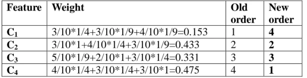
(16) According to TM in Figure 4, the weight of each feature is calculated in the following and the spanning order is thus rearranged.. Feature Weight. Old order 1 2 3 4. 3/10*1/4+3/10*1/9+4/10*1/9=0.153 3/10*1+4/10*1/4+3/10*1/9=0.433 5/10*1/9+2/10*1+3/10*1/4=0.331 4/10*1/4+3/10*1/4+3/10*1=0.475. C1 C2 C3 C4. New order 4 2 3 1. After Creating cleansing tree algorithm is executed, the bitmap indexing matrix TM in 3 with spanned feature order<C4, C2, C3, C1> can be used to generate the cleansing tree. As we can see, the cleansing tree with new feature order O=<C4, C2, C3, C1> in Figure 7 is much smaller than feature order O=<C1, C2, C3, C4> since the explored node are decreased from 15 to 9. Therefore, the computational time of generating and traversal the spanning tree can be largely reduced.. root 1111111111 111. C4. C2. 1 1011100000 110. 4 1010000000 100. 5 0001100000 010. 2 0100000011 110. 6 0100000000 100. 3 0000011100 001. 7 0000000011 110. 8 0000000011 110. C3. 9 0000000011 110. C1. Figure 7. Cleansing tree with feature spanned order <C4, C2, C3, C1>. 16.

(17) We create the cleansing tree with pre-selected feature order by SpanOrder Algorithm. The algorithm, named Creating Cleansing Tree with Discernibility Matrix Algorithm, filling in the class-based discernibility matrix in creating process. The detail algorithms and examples are given as below.. Algorithm 3 Creating cleansing tree with discernibility matrix. Input : A bitmap indexing matrix TM, the valid mask ValidMask,. spanned feature. order O. Output : The valid mask ValidMask, the cleansing tree Tree, a class-based discernibility matrix D.. Step 1: Initialize record[Tree[root]] ← ONEn, class[Tree[root]] ← ONEσm,. Ч 0 , dep← 0 where. weightij← 0 for 1 ≤ i ≤ σm and 1 ≤ j ≤ m-1 and r. dep is the depth of the active node x in the cleansing tree. Step 2: x ← Allocate-Node(), x ←Tree[root]. Step 3: If class[x] = UNIQUEσm or dep = m-1, go to Step 6; otherwise, dep ← dep+1, do the following steps.. Step 4: For each Fjk in Mj, where Mj is the matrix of feature-value vectors of Odep and 1 ≤ k ≤ σj. If record[x] & Fjk.record. Ћ ZERO , do the n. following sub-steps: Step 4.1: y ← Allocate-Node().. Ч 0; otherwise p[y] ← p[x],. Step 4.2: If r= 1, p[y] ← x, left_child[x] ← y, r right_sibiling[x] ← y.. Step 4.3: record[y] ← record[p[y]] & Fjk.record, 17.

(18) class[y] ←BelongToClass(record[y]). Step 4.4: If record[y] ≠ record[p[y]], do the following sub-step: Step 4.4.1: For each bi of class[y], weightij ← weightij+ 1 if bi is equal to 1where 1 ≤ i ≤ σm. Step 4.5: x ← y. Step 5: x ← left_child [p[x]]. Go to Step 3. Step 6: If dep = m-1, do the following steps; otherwise, go to Step 8. Step 7: ValidMask ← record[x] ^ ValidMask. Step 8: If right_sibiling[x]=NIL, x ← p[x], dep ← dep-1 and do Step 9. Otherwise go to Step 10. Step 9: If x=Tree[root], return D, ValidMask and Tree; otherwise go to Step 8. Step 10: x ← right_sibiling[x]. Go to Step 3.. Example 3 For the target table T given in Figure 3, a cleansing tree as shown in Figure 7 can be obtained by applying Creating Cleansing Tree with Discernibility Matrix Algorithm. When creating the tree, it fills in the class-based discernibility matrix D at the same time. As the depth of the tree is one, there are three nodes, 1-st, 2-nd and3-rd nodes, are all spanned by C4. The class value of 1-st node is "110", and the weight14 and in weight24 are increased by one since 1-st node is spanned by C4 which can determine the first and second class. Similarly, the class value of 2-nd node is "110", and the weight14 and in weight24 are all increased by one. The class value of 3-rd node is "001", and weight34 is increased by one. The original class-based discernibility matrix D is shown in Figure 8.. 18.

(19) Cls1. Cls2. Cls3. (C1, 0) (C2, 3) (C3, 0) (C4, 2). (C1, 0) (C2, 2) (C3, 0) (C4, 2). (C1, 0) (C2, 0) (C3, 0) (C4, 1). Figure 8. A class-based discernibility matrix. When any inconsistent record exists, it needs to cleanse the class-based discernibility matrix to ensure no over-weighted. Thus, the Cleansing Discernibility Matrix Algorithm is described as below.. Algorithm 4. Cleansing discernibility matrix. Input: The valid mask ValidMask, spanned feature order O, a class-based discernibility matrix D, the cleansing tree Tree. Output : A class-based discernibility matrix D.. Step 1: x ← Allocate-Node(), x ← left_child[Tree[root]] and dep ← 1 where dep is the depth of the active node x in the cleansing tree. Step 2: If (x = p[x]) go to Step 5; otherwise do the following steps Step 3: If (record[x] & ValidMask) = record[x], go to Step 4; otherwise do the following sub-steps: Step 3.1: diffclass ← BelongToClass (record[x] & ValidMask) ^ class[x]. Step 3.2:. weightij ← weightij -1, if the i-th bit of diffclass is equals to 1, where 1 ≤ i ≤ σm and x is spanned by Odep, is equal to Cj.. Step 3.3: class[x] ← diffclass. Step 3.4: Go to Step 5. Step 4: If class[p[x]] =UNIQUEσm, weightij ← weightij -1, if the i-th bit of 19.

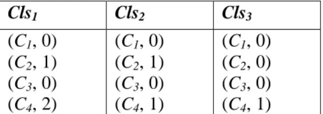
(20) class[x] is equals to 1, where 1 ≤ i ≤ σm and x is spanned by Odep, is equal to Cj. Otherwise go to Step 6. Step 5: If left_child[x] = NIL, go to Step 6; otherwise x ← left_child[x], go to Step 2. Step 6: If right_sibiling[x] = NIL, x ← p[x], dep ← dep-1 and do Step 7. Otherwise go to Step 8. Step 7: If x=Tree[root], return D; otherwise go to Step 6. Step 8: x ← right_sibiling[x]. Go to Step 2.. Example 4 Applying Cleansing discernibility matrix Algorithm on the cleansing tree shown in Figure 7, the class value of 2-th node should be"100" not "110". Thus, the weight24 is decreased by one because of the spanning feature C4 and the second class wrong. Finally, the cleansing class-based discernibility matrix is shown in Figure 9.. Cls1. Cls2. Cls3. (C1, 0) (C2, 1) (C3, 0) (C4, 2). (C1, 0) (C2, 1) (C3, 0) (C4, 1). (C1, 0) (C2, 0) (C3, 0) (C4, 1). Figure 9. A cleansing class-based discernibility matrix. After constructing a class-based discernibility matrix, we can get the feature set by uniting the class-based discernibility matrix. We propose a Union Class-Based Discernibility Matrix Algorithm to do this job.. 20.

(21) Algorithm 5 Union class-based discernibility matrix. Input : A class-based discernibility matrix D Output : The feature set FS. Step 1: For each Clsi in D. Step 2: For each weightij in Clsi. If weightij > 0, FS = FS. ЖC . j. Step 3: Return FS. Example 5 According to Union Class-Based Discernibility Matrix Algorithm, the Cls1 is first examined in D. FS is set to {C4, C2} since both weigh112 weight14 are grater than 0. Similarly, weigh122, weight24 and weigh134 are grater than 0 and FS is a union of {C4}and {C2}, but FS is still {C4, C2}. Thus, {C4, C2} is our solution and feature selection completes.. As mentioned above, we find that the important features can be weighted in class-based discernibility matrix when creating a cleansing tree. The order of feature spanned is determined completely before the creating cleansing tree process, not measured by each node dynamically. Since the measure will be more precise if the feature spanned order is determined in each node, we propose a CurrestBestFeature Algorithm to find the current best feature to span.. Algorithm 6 CurrentBestFeature. 21.

(22) Input : A bitmap indexing matrix TM, current node x, candidate features features. Output : The condition feature Cj. Step 1: Initialize weightj. Ч 0, where 1 ≤ j ≤ m-1.. σ 1 j Count ( F jk .record & x.record ) Step 2: For each Mj in TM, weight j ← ∑ , if n k =1 Count 2 ( F jk .class & x.class). C j ∈ features .. Step 3: Return Cj with max weightj.. Algorithm 7 Creating cleansing tree with discernibility matrix and current best feature. Input : A bitmap indexing matrix TM, the valid mask ValidMask Output : The valid mask ValidMask, the cleansing tree Tree, a class-based discernibility matrix D.. Чʳ ONE , class[Tree[root]]ʳЧʳ ONEσ , weight ← 0 for 1 ≤ i ≤ σ and 1 ≤ j ≤ m-1. rЧ 0. features ←. Step 1: Initialize record[Tree[root]] ij. ʳ. n. m. m. {C-Cm}, where features are the candidate features to span and C is the feature domain of T. path ← ∅, where path is the sequence of spanned features to active node x.. ЧʳAllocate-Node(),ʳx ЧTree[root].ʳ ʳ If class[x] ː UNIQUEσ or dep = m-1, go to Step 7; otherwise, do. Step 2: x Step 3:. m. the following steps.. 22.

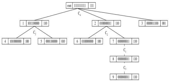
(23) Step 4: Call CurrentBestFeature(x, features) to get Cj, path ←path + Cj, features ← features - Cj, and span all children of x using Mj. Step 5:. For each Fjk in Mj, where 1 ≤ k ≤ σj. If record[x] & Fjk.record. Ћ. ZEROn, do the following sub-steps: Step 5.1: y. ЧʳAllocate-Node().. Ч 0; otherwise p[y] ← p[x],. Step 5.2: If r= 1, p[y] ← x, left_child[x] ← y, r right_sibiling[x] ← y.. Ч record[p[y]] & F .record, class[y] ЧBelongToClass(record[y]).. Step 5.3: record[y]. jk. Step 5.4: If record[y]ʳ Ћ record[p[y]] and the i-th position of class[y] is equals to 1 where 1 ≤ i ≤ σm, weightij ←ʳweightij+ 1. Step 5.5: x Step 6: x. Чʳy.. Чʳleft_child [p[x]]. Go to Step 3.. Step 7: If dep = m-1, do the following steps; otherwise, go to Step 9.. Чʳrecord[x] ^ ValidMask. If right_sibiling[x]= , x Ч p[x], C. Step 8: ValidMask Step 9:. NIL. j. ←last element in path,. features ← features + Cj, and do Step 10. Otherwise go to Step 11. Step 10: If x=Tree[root], return D, ValidMask and Tree; otherwise go to Step 9. Step 11:. x. Чʳright_sibiling[x]. Go to Step 3.. Example 6 According to the Creating cleansing tree with discernibility matrix and current best feature algorithm, it constructs a tree with the order of the feature with currently highest weight. It first counts all feature weight and find the best feature to the root node. According to CurrentBestFeature Algorithm, the weight of C1, C2, C3, C4, is 23.

(24) "0.153", "0.433", "0.331", and "0.475" respectively. Thus, C4 will be selected and we mark each spanning feature in the Figure 10. root 1111111111. 111. C4 1 1011100000 110. 2 0100000011 110. C2. C2. 4 1010000000 100. 5 0001100000 010. 6 0100000000 100. 3 0000011100 001. 7 0000000011 110 C1 8 0000000011 110 C3 9 0000000011 110. Figure 10. Cleansing tree with currently best spanned order. When creating the tree, it fills in the class-based discernibility matrix D at the same time. The class value of 1-st node is "110", and the weight14 and in weight24 are increased by one since 1-st node is spanned by C4 which can determine the first and second class. Similarly, the class value of 2-nd node is "110", and the weight14 and in weight24 are all increased by one since 2-nd node is also spanned by C4. The class value of 3-rd node is "001", and weight34 are increased by one since 3-rd node is spanned by C4 which can determine the third class. The original class-based discernibility matrix D is shown as follows.. Cls1. Cls2. Cls3. (C1, 0) (C2, 3) (C3, 0) (C4, 2). (C1, 0) (C2, 2) (C3, 0) (C4, 2). (C1, 0) (C2, 0) (C3, 0) (C4, 1). According to Cleansing Discernibility Matrix Algorithm, the cleansing class-based discernibility matrix is shown below. 24.

(25) Cls1. Cls2. Cls3. (C1, 0) (C2, 1) (C3, 0) (C4, 2). (C1, 0) (C2, 1) (C3, 0) (C4, 1). (C1, 0) (C2, 0) (C3, 0) (C4, 1). Finally, applying Union Class-Based Discernibility Matrix Algorithm and selected feature set FS is {C4, C2}. Thus, {C4, C2} is our solution and feature selection completes. For the target table T, the solutions of two methods proposed in this section are just the same. In fact, the solutions of them are not always the same.. 4. Experiments. To evaluate the performance of our proposed method, we compare our methods with other feature selection methods. Our target machine is a Pentium III 1G Mhz processor system, running the Microsoft Windows 2000 multithreaded OS. The system includes 512K L2 cache and 256 MB shared-memory.. In these experiments, several datasets are selected from the UCI Repository [12]. We choose datasets with various sorts to test if our method is robust. Some of datasets are with known relevant features (Monks), some are with many classes (SoybeanL), and some are with many instances (Mushroom). Each of them is described briefly as below, and characteristics of the dataset used are shown in Figure 11.. • Monk1, Monk2, Monk3 There are three Monk's problems. The domains for all Monk's problems are the same, which contain six condition features and two classes. Monk1 needs three, 25.

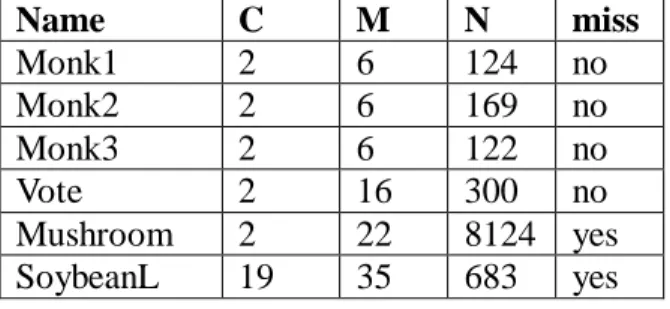
(26) Monk2 needs all six, and Monk3 requires four features to describe the target concepts. These datasets are used to show that relevant features should always be selected.. • Vote This data set includes votes for each of the U.S. House of Representatives Congressmen on the 16 key votes identified by the Congressional Quarterly Almanac (CQA). The dataset consists of 16 condition features, and 300 records.. • Mushroom This data set includes descriptions of hypothetical samples corresponding to 23 species of gilled mushrooms in the Agaricus and Lepiota Family. The dataset consists of 22 condition features, and 8124 records. Each feature can have 2 to 10 values, and there is a feature having missing value.. • SoybeanL The data set has 35 condition features to describe symptoms of 19 different diseases in soybean plant. The values for attributes are encoded numerically, but all have been nominalized. Each feature can have 3 to 6 values, and all but two features have missing values.. Characteristics: name : Database name C : number of classes M : number of condition features N : number of records miss : missing features (yes or no). 26.

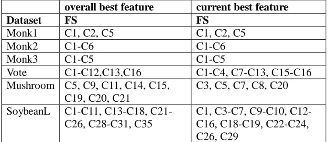
(27) Name Monk1 Monk2 Monk3 Vote Mushroom SoybeanL. C 2 2 2 2 2 19. M 6 6 6 16 22 35. N miss 124 no 169 no 122 no 300 no 8124 yes 683 yes. Figure 11. Experimental Dataset. In the following, the accuracy, number of selected feature set, and time issues will be compared between our methods and the traditional rough set method. The accuracy is measured by exams the classification results of the target table. If the selected feature set can totally solve the problem without any error, 100% accuracy is reached in this dataset; otherwise the accuracy is calculated by the number of records which are successful in classification over the total number of records. At following, we compare our proposed bitmap-based feature selection method with discernibility matrix with different heuristic each other. The heuristics are named as overall best feature and current best feature.. • Accuracy We list the dataset name and the selected features for each method, respectively. Both methods reach the 100% accuracy, and the result is shown in Figure 12. Note that the selected features may result in various combination, we select the first combination that can solve the problem (by alphabetical order) as the selected feature set. The result shows that not all selected features of the two methods are the same, and no definitely subset relation between them exists.. 27.

(28) overall best feature Dataset FS Monk1 C1, C2, C5 Monk2 C1-C6 Monk3 C1-C5 Vote C1-C12,C13,C16 Mushroom C5, C9, C11, C14, C15, C19, C20, C21 SoybeanL C1-C11, C13-C18, C21C26, C28-C31, C35. current best feature FS C1, C2, C5 C1-C6 C1-C5 C1-C4, C7-C13, C15-C16 C3, C5, C7, C8, C20 C1, C3-C7, C9-C10, C12C16, C18-C19, C22-C24, C26, C29. Figure 12. Selected feature set for heuristic solution. • Selected feature set number The selected feature number is shown in Figure 13. Generally speaking, bitmap-based feature selection method with discernibility matrix and current best feature gets the smaller feature set size than bitmap-based feature selection method with discernibility matrix, and that meets our expectation.. Dataset Monk1 Monk2 Monk3 Vote Mushroom SoybeanL. overall best feature 3 6 5 14 8 28. current best feature 3 6 5 13 5 20. Figure 13 Selected feature set number for heuristic solution. • Time In Figure 14, the processing time from cleansing to final output had been evaluated, and the unit is second. The time is rounded to 0 if the real time is less than 0.001 seconds.. 28.

(29) Dataset Monk1 Monk2 Monk3 Vote Mushroom SoybeanL. overall best feature 0 0 0 0 0.01 0.01. current best feature 0 0 0 0 0.02 0.09. Figure 14 CPU time for heuristic solution. It’s surprised that both of our proposed heuristic methods are extremely fast. Even processing the complex dataset such like Mushroom and SoybeanL, the time increases a little. That is good news for us due to the great scalability.. Moreover, we list all proposed methods to evaluate the quality of our proposed heuristic methods. As we can see in Figure 15, the bitmap-based feature selection method with discernibility matrix and bitmap-based feature selection method with discernibility matrix and current best feature result in the larger size of selected features than bitmap-based feature selection method and the traditional rough set, but when is closer to optimal solution.. Dataset. Traditional Bitmap-based RS. Monk1 Monk2 Monk3 Vote Mushroom SoybeanL. 3 6 4 8 4. 3 6 4 8 4 -. Bitmap-based and overall best feature 3 6 5 14 8 28. Bitmap-based and current best feature 3 6 5 13 5 20. Figure 15. The number of selected feature for proposed methods. In addition, we list all proposed methods to evaluate the performance of our proposed heuristic methods in Figure 16. And the more complex the dataset it is, the 29.

(30) more superiority the result shows.. Dataset. Traditional RS. Monk1 Monk2 Monk3 Vote Mushroom SoybeanL. 0.01 0.04 0.01 21.511 225.424 -. Bitmap-based Bitmap-based and overall best feature 0 0 0 0 0 0 1.983 0 21.531 0.01 0.01. Bitmap-based and current best feature 0 0 0 0 0.02 0.09. Figure 16. CPU time of proposed methods. To summarize, the bitmap-based feature selection method with discernibility matrix and current best feature seems to be a method with fast processing time and will get the nearly optimal feature set.. 5. Conclusion and Future Work In this paper, we propose the nearly optimal feature selection method, which employs a discernibility matrix to record the important features during the construction of the cleansing tree to reduce the processing time. And the corresponding indexing and selecting algorithms for such feature selection method are also proposed. Finally, some experiments and comparisons are given and the result shows the efficiency and accuracy of our proposed method. In this paper, a high-speed feature selection method for large dimension space, called bitmap-based feature selection method with discernibility matrix, has been proposed for discovering the nearly optimal feature sets for decision–making problems. Using such selection method, the values of features are not only encoded into bitmap indices for searching the solution efficiently but also using the class-based 30.

(31) discernibility matrix for reducing the searching time. Also, the corresponding indexing and selecting algorithms are described for proposed method. Finally, some experiments are given and comparisons to show the efficiency and accuracy. In the future, the appropriated methodologies to smooth the distinct numeric values to symbolic ones will be further investigated. Moreover, we will attempt to design a mechanism to integrate our proposed methods to evaluate properties of giving dataset and then automatically selects appropriate method for optimal or near-optimal solution.. References [1] R. Barletta, "An introduction to case-based reasoning", AI Expert, Vol. 6, No.8, pp.42-49, 1991. [2] W. C. Chen, S. S. Tseng, J. H. Chen, M. F. Jiang, "A Framework of Feature Selection for the Case-based Reasoning", Proceeding of IEEE International Conference on Systems, Man, and Cybernetics, 2000. [3] W. C. Chen; S. S. Tseng; L. P. Chang, M. F. Jiang, “A Similarity Indexing Method for the Data Warehousing-Bit-wise Indexing Method,” Proceeding of PAKDD 2000, 2000. [4] W. C. Chen; S. S. Tseng; L. P. Chang, T. P. Hong, “A parallelized indexing method for large-scale case-based reasoning,” accepted and to appear in Expert System with Applications, 2002. [5] A. Gonzalez, R. Perez, "Selection of Relevant Features in a Fuzzy Genetic Learning", IEEE Transaction on SMC-Part B, Vol. 31, No. 3, June 2001. [6] M. Last, A. Kandel, O. Maimon, "Information theoretic algorithm for feature selection", Pattern Recognition Letter, Vol. 22, pp.799-811, 2001. [7] H. M. Lee, C. M. Chen, J. M. Chen, Y. L. Jou, "An Efficient Fuzzy Classifier 31.

(32) with Feature Selection Based on Fuzzy Entropy", IEEE Transaction on SMC-Part B, Vol. 27, No. 2, April 1997. [8] H. Liu, R. Setiono, "Incremental Feature Selection", Applied Intelligence 9, pp.217-230, 1998 [9] P. O’Neil; D. Quass, “Improved Query Performance with Variant Indexes,” Proceeding of SIGMOD, Tucson, AZ, May, 1997 [10] Z. Pawlak, "Rough set", International Journal of Computer and Information Sciences, pp.341-356, 1982. [11] Z. Pawlak. "Rough Sets, Theoretical Aspects of Reasoning about Data", Boston, MA: Kluwer Academic Publishers, 1991. [12] J. Quinlan, "Introduction of decision trees", Machine Learning, Vol.1, No. 1, pp.81-106, 1986. [13] M. L. Raymer, W. F. Punch, E. D. Goodman, L. A. Kuhn, "Dimensionality Reduction Using Genetic Algorithm", IEEE Transaction on Evolutionary Computation, Vol. 4, No. 2, July 2000. [14] UCI Repository : http://www.ics.uci.edu/~mlearn/MLRepository.html [15] A. Skowron, C. Rauszer, "The discernibility matrics and functions in information systems", Intelligent Decision Support, pp.331-362, 1992. [16] I. Watson, "Case-based reasoning is a methodology not a technology", Knowledge-Based Systems, Vol. 12, pp.303-308, 1999. [17] M. C. Wu, P. B. Alejandro, "Encoded Bitmap Indexing for Data Warehouses", Data Engineering 1998 Proceedings, pp.220-230, 1998. [18] Y. Yang, T. C. Chiam, "Rule Discovery Based on Rough Set Theory", Information Fusion, FUSION 2000. Proceedings of the Third International Conference on , Vol. 1 , pp. TuC4_11 -TuC4_16, 2000. [19] N. Zhong, J. Dong, S. Ohsuga, "Using Rough Sets with Heuristics for Feature 32.

(33) Selection", Journal of Intelligent Systems, 16, 199-214, 2001.. 33.

(34)