Evaluation of Network Robustness for Given Defense
Resource Allocation Strategies
Y.-S. Lin, P.-H. Tsang
+, C.-H. Chen, C.-L. Tseng, Y.-L. Lin
Department of Information Management
National Taiwan University
Taipei, Taiwan, R.O.C.
{yslin, d91002, r92012, r93002, r93041}@im.ntu.edu.tw
+ Correspondence should be sent to [email protected].
Abstract
Since the 9/11 terrorist attacks, the effective and efficient protection of critical information infrastructures has become an even more important issue. To enhance network survivability, a network operator needs to invest a fixed amount of budget and distribute it properly. However, a potential attacker will always adjust his attack strategies to compromise a network at minimal cost, if he knows the resource allocation strategy of the network operator. In this paper, we first evaluate the survivability of a given network under two different metrics; that is, we assess the minimal attack cost incurred by an attacker. The two survivability metrics are assumed to be the connectivity of at least one given critical Origin-Destination pair (OD pair) and that of all given critical OD pairs. We then analyze the problem with two optimization-based models, in which the problem structure is, by nature, a mixed integer programming problem.
1. Introduction
1.1. BackgroundThe 9/11 terrorist attacks in the United States have led to an increasing global focus on security, especially the effective and efficient protection of infrastructures that are critical to our society. Specifically, the Internet has become a critical information infrastructure since the 1990s. By applying security mechanisms under the defense-in-depth strategy [1], we can enhance the level of robustness. However, the robustness of a network depends not only on each component’s resistance to malicious attacks, but also the network’s topological
structure. The Internet’s topology has been shown to follow a power-law degree distribution [2], and the empirical evidence has highlighted one major weakness: the Internet is highly susceptible to malicious attacks.
With the inevitability of such attacks, perfect robustness of the Internet is unobtainable; hence, in recent years, the concept of security has been increasingly generalized as an issue of survivability. Since there are only two states, safe and compromised, in the context of security [3], the concept is definitely insufficient to fully describe how a system can sustain normal services under abnormal conditions, including random errors and malicious attacks. Consequently, the issue of survivability has drawn increasing attention in recent years [4, 5].
1.2. Related works of survivability
Despite the rapid increase in survivability research, the definition of survivability is anything but clear [6]. Since it is impossible, in practice, to build a perfectly survivable network, it is important to be able to quantitatively evaluate the efficacy of a network that is believed to be survivable. From our survey, methods that attempt the quantitative analysis of survivability can be classified into two categories: connectivity or performance.
The analysis of network connectivity is based on two factors: the Node Connectivity Factor (NCF) [7] and the Link Connectivity Factor (LCF) [8]. The former deals with the removal of nodes, while the latter is concerned with the removal of links. Several methodologies can be used to analyze the connectivity of networks. Among them, linear/non-linear programming [8] and simulation with given metrics [7] are the most popular.
In general, network performance is analyzed by calculating the probability that the network will fulfill its given QoS metrics. Because of the variety of network performance metrics, many diverse methodologies, such as Markov chain [5], game theory [9] and simulation with given metrics [10], can be used for analysis.
1.3. Motivation and objectives of this paper To enhance network survivability effectively, a network operator must invest a fixed amount of budget (e.g. money, time, and manpower) and distribute it properly. On the other hand, an attacker also has limited resource to launch an attack, so he won’t choose to compromise a network if the incurred attack cost exceeds his acceptable level. Thus, a potential attacker will always adjust his strategies to compromise a network at minimal cost, if he knows the defense resource allocation strategy of the network operator.
In this paper, to understand how well a network can sustain malicious attacks, we evaluate the minimal attack cost incurred by an attacker who attempts to disconnect critical Origin-Destination pair(s) (OD pair(s)). The concept of attack cost relates to the effort an attacker needs to make to attain his goal. However, to the best of our knowledge, no mathematical model that deals with defense and attack behavior in the context of survivability has been proposed. We therefore propose two mathematical models that fully describe the conflict between an attacker and a defender, and show different levels of network survivability for given defense resource allocation strategies. Briefly, Model 1 deals with the disconnection of at least one critical OD pair in a network, while Model 2 addresses the disconnection of all critical OD pairs in a network.
1.4. Outline of this paper
The remainder of this paper is organized as follows. In Section 2, a min mathematical formulation of an attack-defense scenario is proposed, which is later shown to be a trivial problem. In Section 3, another min mathematical formulation of an advanced attack-defense scenario is proposed, for which a Lagrangean Relaxation-based solution approach is presented. In Section 4, the computational results of the second formulation are reported. Finally, in Section 5, we present our conclusions.
2. Problem formulation for model 1
2.1. Problem descriptions and assumptionsThe evaluation of the robustness of a network under malicious attack is modeled as an optimization problem, in which the objective is to minimize the total attack cost from an attacker’s perspective, such that at least one given critical OD pair is disconnected and the network cannot survive.
In this model, we assume that both the attacker and the defender have complete information about the targeted network topology. Moreover, the attacker has complete information about the defender’s budget allocation. For simplicity, we only consider node attacks, which result in the worst case scenarios and are more common in the real world.
We now define the notations used in this paper and formulate the problem.
Table 1. Given parameters Notation Description
V The index set of all nodes
L The index set of all links
W The index set of all given critical origin-destination pairs
OUT i The index set of outgoing links of node i,
where i V∈
M A large number that represents the link disconnection
ε
A small number that represents the link connectednessw
P
The index set of all candidate paths of an OD pair w, where w W∈δpl An indicator function, which is 1 if link l
is on path p, and 0 otherwise (where
l L∈ , p P∈ w)
bi Budget allocated to node i, which is also
the threshold of an attack cost leading to a successful attack, where i V∈
Table 2. Decision variables Notation Description
yi 1 if node i is compromised, and 0
otherwise (where i V∈ )
wl
t
1 if link l is used by an OD pair w, and 0 otherwise (where l L∈ , w W∈ )xp 1 if path p is chosen, and 0 otherwise
(where p P∈ w)
l
c
Cost of link l, where l L∈Objective function: min i i i y
∑
i V∈ y b , (IP 1) subject tol i c =y M+ε ∀ ∈i V l OUT, ∈ i (IP 1.1) wl l pl l l L l L t c δ c ∈ ≤ ∈
∑
∑
∀ ∈p P w Ww, ∈ (IP 1.2) w p pl wl p P x δ t ∈ =∑
∀ ∈
w W l L
,
∈
(IP 1.3) wl l l L w W M t c ∈ ∈ ≤∑ ∑
(IP 1.4) 1 w p p P x ∈ =∑
∀ ∈
w W
(IP 1.5) 0 or 1 p x = ∀ ∈p P w Ww, ∈ (IP 1.6) 0 or 1 i y = ∀ ∈i V (IP 1.7) 0 or 1 wl t =∀ ∈
w W l L
,
∈
(IP 1.8) or l c =ε M +ε ∀ ∈ l L. (IP 1.9) The objective of this formulation is to minimize the total attack cost. Constraint (IP 1.1) describes the definition of the link cost, which isε
if the link functions normally, and M+ε
if it is broken. Constraint (IP 1.2) requires that the selected path for each OD pair, w, should be the minimum cost path. Constraint (IP 1.3) is the relation among twl, xp and δpl.We use the auxiliary set of decision variables, twl, to
replace the sum of all xpδpl. Constraint (IP 1.4) requires
that at least one critical OD pair is disconnected. We depict the phenomenon by showing that the sum of the shortest path costs for each OD pair to communicate is greater than M. Constraint (IP 1.9) is a set of redundant constraints, since the value of each cl should be
either
ε
or M+ε
.Argument 1 We can relax the equality of Constraint (IP 1.1) as cl ≤y Mi +ε without affecting the
optimality conditions.
Argument 2 We can relax the equality of Constraint (IP 1.3) as w p pl wl
p P
xδ t ∈
≤
∑ without affecting the optimality conditions.
2.2. Solution to model 1
Lemma 1 Given a budget allocation strategy, a topology, G= (V, L), and a set of critical OD pairs, W, the formulation of Model 1 can be optimally solved by combining the maximum flow-minimum cut algorithm [11] and the node splitting method [11] within time complexity O(|W|¯(|V|+|L|)¯n), where n is the total budget allocated to the network.
Proof. The maximum flow-minimum cut algorithm
finds the minimum link cost that separates the network into two subsets, where the origin node belongs to subset S and the destination node belongs to subset S . With the node splitting method, on the other hand, a node can be converted into a link by dividing it into
two independent subnodes and introducing an artificial link to connect the subnodes. By assuming that the link capacity between two subnodes of a node is the given budget (i.e., the attack cost) of the node and other links’ capacities are infinite, we first transform G(V, L) into G’(V’, L’). Using the maximum flow-minimum cut algorithm, the minimum cost of separating G’ into two subsets for OD pair w, where w W∈ , can then be denoted by MCTw, which is also the minimum cut for OD pair w in G’. Since the network contains |W| critical OD pairs, we can find the minimum cost for each OD pair after running the maximum flow-minimum cut algorithm |W| times. Thus, the solution to Model 1 is min(MCTw), where w W∈ . Meanwhile, the time complexity of the maximum flow-minimum cut algorithm is O((|V|+|L|)¯n), and the time complexity of solving Model 1 optimally is O(|W|¯(|V|+|L|)¯n), where n is the total capacity (not including the infinite capacity), i.e., the total defense budget, of the network.
3. Problem formulation for model 2
3.1 Problem descriptions and assumptionsWe now consider another scenario of the attack-defense problem. Assume that an attacker must disconnect all given critical OD pairs to compromise a network.
The given parameters and decision variables of Model 2 are the same as those of Model 1, except that a new given parameter, B, which is the total budget of a defender, is introduced. The objective of this formulation (IP2) and the constraints (IP 2.1)~(IP 2.10) of Model 2 are the same as those for Model 1, except the two following constraints.
wl l l L M t c ∈ ≤
∑
∀ ∈w W (IP 2.4) i lb i V y V ∈ ≥∑
(IP 2.10) Constraint (IP 2.4) requires that all critical OD pairs must be disconnected. We explain the phenomenon by showing that the cost of the shortest path for each OD pair to communicate is greater thanM. Constraint (IP 2.10) is a redundant constraint. We find a legitimate lower bound, Vlb , which is the
number of nodes an attacker must target to compromise the connectivity of all critical OD pairs. Argument 3 The legitimate lower bound described in Constraint (IP 2.10) can be obtained by the following method.
We assign one unit of the budget to each node. Then, we solve this revised optimization problem and find a lower bound of the Lagrangean Relaxation (LR) method [12], denoted by LB, on the optimal objective function value. LB indicates the minimal (but not necessarily feasible) cost an attacker must expend to achieve his goal. Since each node is assigned one unit of the budget, LB also serves as the lower bound of the number of nodes an attacker needs to compromise. 3.2. Solution to model 2
By applying the Lagrangean Relaxation method with a vector of Lagrangean multipliers, we can transform the problem of (IP2) into the following Lagrangean Relaxation problem (LR), where constraints (IP 2.1), (IP 2.2), (IP 2.3), and (IP 2.4) are relaxed.
Lagrangean Relaxation Problem
1 1 2 3 4 2 3 4 ( , , , ) min [ ( )] [ ] [( ) ] i i w w D y i i il l i i V i V l OUT wp wl l pl l wl p pl wl w wl l w W p P l L w W l L p P w W l L Z u u u u y b u c y M u t c c u x t u M t c ε δ δ ∈ ∈ ∈ ∈ ∈ ∈ ∈ ∈ ∈ ∈ ∈ = + − + + − + − + − ∑ ∑ ∑ ∑ ∑ ∑ ∑∑ ∑ ∑ ∑ (LR) subject to 1 w p p P x ∈ =
∑
∀ ∈w W (LR1) 0 or 1 p x = ∀ ∈p P w Ww, ∈ (LR2) 0 or 1 i y = ∀ ∈i V (LR3) 0 or 1 wl t = ∀ ∈w W l L, ∈ (LR4) or l c =ε M+ ε ∀ ∈l L (LR5) . i lb i V y V ∈ ≥∑
(LR6) By definition, u u u u1, , ,2 3 4 are the vectors of {u1il},{u2
wp}, {u3wl}, {u4w}, respectively. Note that
1, , ,2 3 4
u u u u are Lagrangean multipliers and 1, , ,2 3 4
u u u u ≥0 . To solve (LR) optimally, we decompose it into the following three independent and easily solvable optimization subproblems.
Subproblem 1 SUB_1 (related to decision variable xp) 3 1( ) min3 w sub wl pl p w W l L p P Z u u δ x ∈ ∈ ∈ =
∑ ∑ ∑
, (Sub 1) subject to (LR1) and (LR2).This problem can further be decomposed into |W| independent minimum cost path subproblems. In other words, we can determine the value of xp individually
for each OD pair. Due to the non-negativity constraint of each u3
wl, which can be treated as the cost of link l in
OD pair w in the minimum cost path subproblems, we can apply Dijkstra’s shortest path algorithm to solve these subproblems optimally. The time complexity of SUB_1 is O(|W|¯|V|2).
Subproblem 2 SUB_2 (related to decision variable y ) i 1 2( ) min1 ( ) i sub i i il i i V i V l OUT Z u y b u M y ∈ ∈ ∈ =
∑
+∑ ∑
− , (Sub 2) subject to (LR3) and (LR6).To solve SUB_2 optimally, we first apply the quick sort algorithm to the sum of the parameters of each yi
to obtain an array in ascending order. To satisfy Constraint (LR6), we choose Vlbnodes from the left of
the array, and set their yi values to one. The yi values of
the remaining nodes are decided by their associated parameters. If it is positive, the value of yi is set to zero
to minimize this subproblem; otherwise, it is set to one. The time complexity of SUB_2 is O(|V|log|V|). Subproblem 3 SUB_3 (related to decision variables ,t cwl l) 1 2 3 1 2 3 4 3 4 ( , , , ) min ( ) ( ) ( ) i w sub il l wp wl l pl l i Vl OUT w W p P l L wl wl w wl l w W l L w W l L Z u u u u u c u t c c u t u t c δ ∈ ∈ ∈ ∈ ∈ ∈ ∈ ∈ ∈ = + − + − + −
∑ ∑
∑ ∑ ∑
∑∑
∑
∑
(Sub 3) subject to (LR4) and (LR5).As Constraints (LR4) and (LR5) show, twl and cl
have two combinations each. We can therefore apply an exhaustive search to determine the values of twl and
cl, depending on which combination derives the
smallest objective function value. To optimally solve SUB_3, we further decompose it into |L| independent subproblems. The time complexity of SUB_3 is O(|W|¯|L|).
According to the weak Lagrangean duality theorem [12], the optimal value of the Lagrangean Relaxation (LR) problem is, by nature, a lower bound (for minimization problems) of the objective function value in the primal problem. The tightest Lagrangean lower bound can be derived by tuning the Lagrangean multipliers, i.e., by maximizing the LR problem. There are several methods for solving this problem, of which the Subgradient optimization technique [13] is the most popular.
Getting Primal Feasible Solutions
To obtain the primal feasible solutions of (IP2), we consider the solutions of the LR problem. By using the Lagrangean Relaxation method and the Subgradient method to solve the LR problem, we not only get a theoretical lower bound on the primal objective function value, but also obtain good hints for getting primal feasible solutions. However, as some critical and difficult constraints are relaxed to obtain the easily-solvable LR problem, the solutions obtained from ZD may not be valid for the primal problem. Thus, we need to develop good heuristics to tune the values of the decision variables, so that primal feasible solutions can be obtained. Our proposed heuristics are as follows.
Table 3. Algorithm for getting a primal feasible solution
Sort the array of nodes in ascending order according to the associated parameters of yi in SUB_2;
INIT all yi to 0;
FOR (each unexamined node i in the array with the smallest parameter) {
IF (there is an available path for at least one given critical OD pair to communicate)
IF (the parameter of yi < 0 OR the node’s
outgoing link cost is greater than M) SET yi to 1;
}
/* recovery of the attack behavior to reduce ineffective attacks */
FOR (each attacked node i with the largest budget, bi)
{
SET yi to 0;
IF (there is an available path for at least one given critical OD pair to communicate)
SET yi to 1;
}
FOR (any two combinations, i and j, of the attacked nodes) {
SET yi and yj to 0;
IF (there is an available path for at least one given critical OD pair to communicate)
SET yi and yj to 1;
}
The time complexity for getting primal heuristics is
O(|W|¯|V|5).
4. Computational experiments
To demonstrate that our proposed solution to Model 2 is better than other approaches, we implement the following two simple algorithms for comparison. 4.1. Simple algorithm 1
Table 4. Simple algorithm 1 FOR (each OD pair)
Run Maximum Flow-Minimum Cut algorithm to get the minimum cuts;
FOR (each node that belongs to any of the minimum cuts AND contains at least one outgoing link labeled as M) {
Run Dijkstra’s Shortest Path algorithm under the node’s recovery;
IF (the recovery of the node is unallowable) Un-recover the node;
}
4.2. Simple algorithm 2
Table 5. Simple algorithm 2
Sort the nodes in descending order according to their degree of connectivity;
WHILE (there is an available path for at least one OD pair to communicate)
Attack the most connected node among those that have not been attacked;
4.3. Experimental parameters and cases
We present our experimental parameters and the design of cases in the following table.
Table 6. Experimental parameters Number of Nodes 16, 50, 100
Number of Links 60 ~ 400 Number of Critical
OD Pairs 8 ~ 250
Testing Topology Random Networks (RN) Grid Networks (GN) Scale-free Networks (SN) [14] Initial Budget
Allocation Strategy Uniform Distribution Degree-based Distribution Number of Iterations 2000
Non-improvement
Counter 80
Initial Upper Bound Solution of Simple Algorithm 1 4.4. Experimental results
We present the experimental results in the appendix section and show the figures below. SA1 and SA2 are the solutions obtained by the Simple Algorithms 1 and 2; the LR value represents the primal feasible solution derived by the LR process; and LB represents the lower bound gained from the LR process. The duality gap is calculated by LR-LB*100%
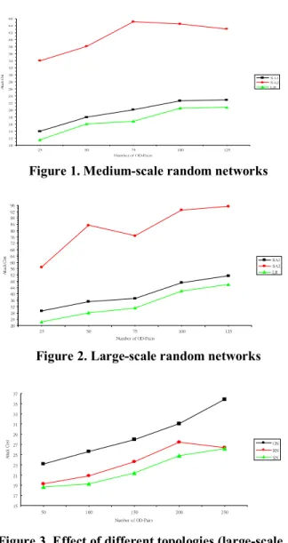
10 12 14 16 18 20 22 24 26 28 30 32 34 36 38 40 42 44 46 25 50 75 100 125 Number of OD-Pairs At ta ck C os t SA1 SA2 LR
Figure 1. Medium-scale random networks
20 24 28 32 36 40 44 48 52 56 60 64 68 72 76 80 84 88 92 96 25 50 75 100 125 Number of OD-Pairs A tt ack C os t SA1 SA2 LR
Figure 2. Large-scale random networks
15 17 19 21 23 25 27 29 31 33 35 37 50 100 150 200 250 Number of OD-Pairs A tt ack C o st GN RN SN
Figure 3. Effect of different topologies (large-scale networks with a uniform budget allocation strategy)
20 22 24 26 28 30 32 34 36 38 40 42 44 46 48 50 100 150 200 250 Number of OD-Pairs A tt ack C o st GN RN SN
Figure 4. Effect of different topologies (large-scale networks with a degree-based budget allocation
strategy) 4.5. Discussion
From Figures 1 and 2, we observe that the curves of the LR-based algorithms are all below those of SA1
and SA2, which means that the solution quality of LR is better than those of SA1 and SA2, because this is a minimization problem. Specifically, the solution excellence of the LR-based algorithm is demonstrated when a network’s size increases and more OD pairs are considered.
Since a legitimate lower bound of the primal objective function value (LB) can be obtained by Lagrangean Relaxation, we can also evaluate the solution quality of LR by comparing it with the LB. We find that even in a medium-scale network or large-scale network, the duality gap, in most cases, is less than 45%.
Moreover, we find that a network’s topological structure strongly influences its robustness against attack. Figure 3 shows the minimal attack costs of different network topologies under a uniform budget allocation strategy with the same network size and number of critical OD pairs. Clearly, cost of attacking a random network is greater than that of attacking a scale-free network. This indicates that the property of randomness may help maintain the connectivity of a network. The connectivity of a scale-free network is usually maintained by a few super nodes. However, since an attacker will try to destroy nodes that have a high degree of connectivity to achieve his goal more easily, the effect of destroying some super nodes would be significant. Therefore, the robustness of a scale-free network is weaker than that of a random network, since it can be shut down completely by compromising fewer nodes than in a random network.
If we compare Figure 3 with Figure 4, we can see that a proper budget allocation strategy enhances the robustness of a network. By adjusting the budget allocation strategy according to the degree of connectivity, a scale-free network can achieve the higher level of robustness than a random network most of the time, as shown in Figure 4. Thus, if we allocate proper budgetary resources to high-connectivity nodes, we can increase the costs incurred by an attacker.
5. Conclusions
In this paper, we have focused on two issues. First, we have discussed the robustness of a network and evaluated the minimal attack cost of an attacker based on two different survivability metrics: the connectivity of at least one OD pair, and the connectivity of all critical OD pairs. Second, we have presented one lemma, which shows a pseudo-polynomial time solution approach to solve Model 1 optimally.
One of the major contributions of our paper is the mathematical models. We have researched the problem characteristics carefully, identified the problem objectives and the associated constraints, and proposed
well-formulated mathematical models. To the best of our knowledge, this paper is the first to model attack-defense scenarios as mathematical programming problems in the context of survivability. Furthermore, we have provided solution approaches to find the minimal attack cost for both models, and derived a legitimate lower bound on the number of nodes an attacker would need to target in Model 2. The proposed lemma is another major contribution. After studying the problem structure of Model 1, we find trivial solution for the problem and present it as elegant lemma.
Finally, we have evaluated different topologies and observed their ability to maintain the connections of all critical OD pairs under malicious attack. The experimental results show that a random network can survive better than a scale-free network. However, with a proper budget allocation strategy, a scale-free network can achieve the higher level of robustness than a random network most of the time.
We believe that our modeling techniques can be extended to different attack-defense scenarios in the context of survivability in which the survivability metrics include “any number of given critical OD-pairs are disconnected,” “a single core node is survivable,” or “multiple core nodes are survivable.” Besides considering the state of a node is compromised or not merely, we could lead into the concept of probability to define the likelihood of a node being properly functional. We are also interested in the extent to which our methods can be extended to scenarios with the interactive dependency of network nodes, and specific application parameters of wireless networks, mobile phone networks, and other kinds of network environment.
References
[1] “Information Assurance Technical Framework (IATF)
Release 3.1:2002”, National Security Agency (NSA), http://www.iatf.net/framework_docs/version-3_1/.
[2] Q. Chen, H. Chang, R. Govindan, S. Jamin, S. J.
Shenker, and W. Willinger, “The Origin of Power Laws in Internet Topologies Revisited”, Proceedings of the 21th Annual Joint Conference of the IEEE Computer and Communications Societies (INFOCOM ’02), Volume 2, 2002, pp. 608-617.
[3] R. J. Ellison, D. A. Fisher, R. C. Linger, H. F. Lipson, T. A. Longstaff, and N. R. Mead, “Survivable Network Systems: An Emerging Discipline”, Technical Report CMU/SEI-97-TR-013, Software Engineering Institute, Carnegie Mellon University, November 1997 (Revised: May 1999).
[4] J. C. Knight, E. A. Strunk, and K. J. Sullivan, “Towards a Rigorous Definition of Information System Survivability”, Proceedings of the DARPA Information Survivability Conference and Exposition
(DISCEX 2003), Volume 1, April 2003, pp.78-89. [5] Y. Liu and K. S. Trivedi, “A General Framework for
Network Survivability Quantification”, Proceedings of the 12th GI/ITG Conference on Measuring, Modeling and Evaluation of Computer and Communication Systems, September 2004.
[6] V. R. Westmark, “A Definition for Information
System Survivability”, Proceedings of the 37th IEEE Hawaii International Conference on System Sciences, Volume 9, 2004, p. 90303.1.
[7] R. Albert, H. Jeong, and A.-L. Barabási, “Error and
Attack Tolerance of Complex Networks”, Nature,
Volume 406, July 2000, pp. 378-382.
[8] N. Garg, R. Simha, and W. Xing, “Algorithms for
Budget-Constrained Survivable Topology Design”, Proceedings of the 2002 IEEE International Conference on Communications, Volume 4, 2002, pp. 2162-2166.
[9] S. Kumar and V. Marbukh, “A Game Theoretic
Approach to Analysis and Design of Survivable and Secure Systems and Protocols”, Proceedings of the 2nd International Workshop on Mathematical Methods, Models, and Architectures for Computer Network Security, LNCS 2776, September 2003, pp. 440-443. [10] W. Molisz, “Survivability Function—A Measure of
Disaster-Based Routing Performance”, IEEE Journal on Selected Areas in Communications, Volume 22, Issue 9, November 2004, pp. 1876-1883.
[11] R. K. Ahuja, T. L. Magnanti, and J. B. Orlin, Network Flows, 1993, pp. 41-42, 184-191, 598-648.
[12] M. L. Fisher, “The Lagrangean Relaxation Method for Solving Integer Programming Problems”, Management Science, Volume 27, Number 1, January 1981, pp. 1-18.
[13] M. Held, P. Wolfe, and H. P. Crowder, “Validation of
Subgradient Optimization”, Mathematical
Programming, Volume 6, 1974, pp. 62-88.
[14] A.-L. Barabasi and R. Albert, “Emergence of Scaling in Random Networks”, Science, Volume 286, October 1999, pp. 509-512.
Appendix
Case 1: Small-scale (16-node) networks with degree-based budget distribution
Network Topology
No. of Critical
OD pairs SA1 SA2 LR LB Duality Gap
8 4.33 16 4.33 4.1286 4.88% 16 7.33 16 7.33 6.639864 10.40% 24 7.33 16 7.33 6.833638 7.26% 32 10.33 16 10.33 9.147548 12.93% Grid Networks 40 12.33 16 12.33 10.2583 20.20% 8 5.2 9.8 5.066667 4.363142 16.51% 16 7.4 12.93333 6.8 5.579946 21.81% 24 8.266667 14.46667 7.866667 6.813326 16.22% 32 9.666666 14.26667 9.066666 7.604745 19.43% Random Networks 40 9.2 15 9 7.820135 14.88% 8 6.62069 11.2 6.179311 5.118475 21.79% 16 8.331034 13.46207 7.944828 6.760865 18.26% 24 8.827586 13.68276 8.717241 7.424418 17.60% 32 10.2069 14.12414 9.875862 7.924543 25.12% Scale-free Networks 40 10.48276 14.78621 10.26207 8.535546 20.32%
Case 2: Medium-scale (50-node) networks with degree-based budget distribution
Network Topology
No. of Critical
OD pairs SA1 SA2 LR LB Duality Gap
25 13.23912 39.52071 11.66706 8.67917 34.39% 50 22.22557 41.89881 19.73563 14.72979 34.14% 75 21.29319 46.7002 19.60321 13.89132 41.15% 100 19.52173 43.6905 18.89996 14.45762 31.03% Grid Networks 125 21.01724 47.04804 20.29598 14.99273 35.42% 25 14 14 11.6 9.531583 21.68% 50 18 18 16.06667 12.88349 24.76% 75 20.2 20.2 16.8 13.47968 24.81% 100 22.66667 22.66667 20.6 16.81728 22.84% Random Networks 125 22.93333 22.93333 20.8 16.36455 27.22% 25 15.56701 37.62887 14.94845 12.38963 21.05% 50 22.62887 42.42268 19.79381 16.06501 23.91% 75 25.05155 42.78351 22.83505 17.6532 29.75% 100 25.30928 45.36082 23.71134 19.00001 24.76% Scale-free Networks 125 26.64948 43.29897 25.46392 20.68265 23.29%
Case 3: Large-scale (100-node) networks with degree-based budget distribution
Network
Topology No. of Critical OD pairs SA1 SA2 LR LB Duality Gap
50 32.84444 94.7 23.10222 16.52974 39.78% 100 32.63335 96.52222 26.21112 18.65637 40.56% 150 32.93333 97.17775 29.28888 20.88303 40.30% 200 38.11555 98.63332 32.84445 21.65815 51.87% Grid Networks 250 40.69554 95.20222 37.17778 23.6082 57.52% 50 29.4 56.93333 22.40465 17.7652 25.65% 100 35.2 83.66667 28.06667 21.54525 30.22% 150 37.26667 76.86667 31.2 24.18611 29.17% 200 47.2 93.2 42 29.81787 40.92% Random Networks 250 51.6 95.6 46 37.51661 22.65% 50 35.32995 78.4264 32.08122 24.07327 33.35% 100 44.77157 85.58376 40.05076 30.69447 30.62% 150 45.73604 83.85787 40.50761 30.70721 32.20% 200 49.3401 94.72081 44.8731 34.59037 29.84% Scale-free Networks 250 50.10152 97.96954 44.51777 35.32274 26.12%