國
立
交
通
大
學
生醫工程研究所
碩
士
論
文
利 用 情 感 性 視 覺 誘 發 腦 磁 波 之 情 緒 辨 識
Emotion Recognition using Magnetoencephalographic
Recordings Evoked by Affective Visual Stimuli
研 究 生:李欣芳
指導教授:陳永昇 博士
利 用 情 感 性 視 覺 誘 發 腦 磁 波 之 情 緒 辨 識
Emotion Recognition using Magnetoencephalographic
Recordings Evoked by Affective Visual Stimuli
研 究 生:李欣芳 Student:Hsin-Fang Lee
指導教授:陳永昇 Advisor:Yong-Sheng Chen
國 立 交 通 大 學
生 醫 工 程 研 究 所
碩 士 論 文
A ThesisSubmitted to Institute of Biomedical Engineering College of Computer Science
National Chiao Tung University in partial Fulfillment of the Requirements
for the Degree of Master
in
Computer Science August 2011
Hsinchu, Taiwan, Republic of China
近年來因為情緒和壓力造成的情感性疾病逐年增加,如能讓智慧型環境系統偵測 我們的情緒,當偵測到負面情緒時,系統能夠適時的改變週遭的環境,如光線、 溫度、音樂等,讓我們的情緒能因環境的舒適而改善,將有助於降低情感性疾病 的發生。因此情緒的辨識系統變得越來越重要,關於情緒辨識的各方面研究也在 近幾年內蓬勃發展。在情緒辨識的領域上,過去大都採用臉部表情、語音及肢體 語言等外在表徵來辨識情緒,本研究提出一個基於腦磁波訊號的情緒辨識系統, 採用情感性視覺刺激的誘發,觀察腦磁波訊號中所呈現出的腦波變化來進行情緒 辨識。本情緒辨識系統分為生理訊號的擷取、特徵擷取、分類三個主要部份,本 研究共收集 14 位正常人與 14 位憂鬱症患者,並使用五種特徵擷取方法,分別為 事件相關磁場(event-related magnetic fields, ERF)、頻譜能量密度(power spectral density, PSD)、自迴歸模型(autoregressive (AR) model)、主成分分析(principal component analysis, PCA)、以及局部線性嵌入(locally linear embedding, LLE),經 比較這些特徵擷取方法後,我們採用結合頻譜能量密度的頻域特徵與局部線性嵌 入的空間降維,並利用支持向量機 (support vector machine, SVM)來進行情緒分 類。實驗結果顯示,我們的情緒辨識系統在分辨快樂和害怕這兩種情緒時,平均 準確率能達到 91.8%。因此,在腦波特徵擷取上,頻譜能量密度與局部線性嵌入 的結合,可以達到不錯的辨識率。
Abstract
The prevalence of affective disorders has been increasing recently. One
possible remedy is to construct an intelligent environment system which
can recognize emotions and adjust the conditions of environment like
temperature, light, and music to comfort the subjects when their negative
emotions are detected. Therefore, automated emotion recognition has
attracted more and more attentions in the field of affective computation.
In the literature, there have been many research works which recognize
emotions through external manifestation, such as facial expression, voice,
and gestures. In this works, we propose an emotion recognition system
using magnetoencephalographic (MEG) signals evoked by affective
visual stimuli. Our system can be divided into three parts including
physiological signal acquisition, feature extraction, and classification. We
recruited 14 normal subjects and 14 bipolar disorder patients. Five kinds
of feature extraction methods were evaluated in this work, including:
event-related magnetic fields (ERF), power spectral density (PSD),
autoregressive (AR) model, principal component analysis (PCA), and
locally linear embedding (LLE). We adopted the features and the
combination of PSD and LLE as use support vector machine (SVM) to
categorize happy and fear emotions. According to our experiments, the
proposed system can achieve 91.8% accuracy of emotion recognition.
這七百多個日子裡,感謝許多人給予的幫助與鼓勵。 感謝陳永昇老師和陳麗芬老師在我的研究生涯裡,不僅在研究上耐心的給予 教導,在上活上也會適時的給予關心,讓我們能無憂無慮的專心做研究。 感謝口試委員-王才沛老師和王振興老師,提供了寶貴的意見與指導,讓我 學習到更多的東西,也讓論文更加完整。 感謝小白學長,在研究上,當我遇到難題時,總是會給我一些建議和協助。 感謝 BSP Lab 一起奮鬥的夥伴們-阿爆、乙宛、國維、蓮霧,一路上互相扶 持砥礪,在我最後關頭時,當我流淚最沮喪的時候,因為有你們的陪伴,讓我可 以擦乾淚水繼續堅持的力量,還有慧玲學姊、詠成學長、小苑學姊、Sheep 學長、 小艾以及學弟妹們,因為有你們的陪伴與幫助,讓我的研究生活過得很精彩,充 滿許多回憶。 最後,要感謝我摯愛的家人,當我遇到困難時,因為有你們的支持與鼓勵, 讓我有繼續走下去勇氣,也因此才能夠順利的完成碩士學位。
Emotion Recognition using
Magnetoencephalographic Recordings Evoked
by Affective Visual Stimuli
A thesis presented by
Hsin-Fang Lee
to
Institute of Biomedical Image and Engineering
College of Computer Science
in partial fulfillment of the requirements for the degree of
Master
in the subject of
Computer Science
National Chiao Tung University Hsinchu, Taiwan
Copyright © 2011 by
Contents
List of Figures v
List of Tables vii
1 Introduction 1 1.1 Motivation . . . 2 1.2 Thesis scope . . . 3 1.3 Thesis organization . . . 5 2 Related works 7 2.1 Emotion psychology . . . 8
2.1.1 The definition of emotion . . . 8
2.1.2 The theory of emotion . . . 8
2.1.3 The category of emotion . . . 9
2.2 Physiological signals . . . 11
2.2.1 Autonomic nervous system and peripheral nervous system . . . 11
2.2.2 Central nervous system . . . 14
2.3 Feature extraction . . . 15
3 Classification of affective evoked brain activities 17 3.1 Materials . . . 19 3.1.1 Participants . . . 19 3.1.2 Experimental paradigm . . . 19 3.1.3 MEG device . . . 20 3.1.4 Neurophysiological recordings . . . 22 3.1.5 Data preprocessing . . . 22
3.2 Feature extraction (feature generation) . . . 22
3.2.1 Event-related magnetic fields . . . 22
3.2.2 Power spectral density . . . 26
3.2.3 Autoregressive model . . . 26
3.2.4 Principal component analysis . . . 27 iii
3.4 Classification . . . 32
3.4.1 Support vector machine . . . 32
3.4.2 Evaluation . . . 35
4 Experiment results 37 4.1 Preprocessing results . . . 38
4.2 Results of all participants . . . 39
4.3 Results of gender difference participants . . . 39
4.4 Results of BD patients . . . 39
5 Discussion 49 5.1 Classification using emotions or conditions? . . . 50
5.2 Behavioural results . . . 50
5.3 Effects of on the number of trials accuracy . . . 57
6 Conclusions 65
Bibliography 67
List of Figures
1.1 Physiological signals-based emotion recognition. . . 4
2.1 Plutchik’s three-dimensional emotion mode [25]. . . 10
2.2 Russell’s two-dimensional emotion mode [25]. . . 10
2.3 Thayer’s two-dimensional emotion mode [25]. . . 11
2.4 Kim, K. H et al. development of emotion recognition system [13]. . . 13
2.5 Kim, J. and Andre, E. development of supervised statistical classification system for emotion recognition [12] . . . 14
2.6 The 2-D emotional space [14]. . . 15
3.1 Framework of this thesis. . . 18
3.2 The experiment paradigm of emotion recognition. . . 20
3.3 The MEG device in Taipei Veterans General Hospital. . . 21
3.4 Preprocessing procedures for MEG. . . 23
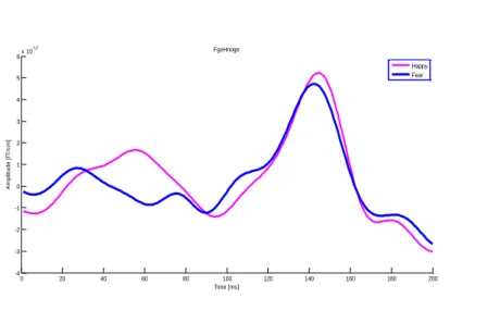
3.5 Waveforms of mean ERF regional amplitudes evoked by FgoHnogo condi-tion. . . 24
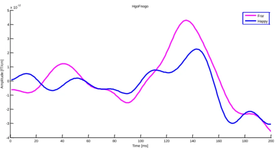
3.6 Waveforms of mean ERF regional amplitudes evoked by HgoFnogo condi-tion. . . 25
3.7 The example of nonlinear dimensionality reduction as illustrated for data (B) sampled from a two dimensional manifold (A). By way of nonlin-ear dimensionality reduction algorithm (LLE), the data is mapped to two-dimensional space (C) [23]. . . 29
3.8 Steps of locally linear embedding [21]. . . 30
3.9 SVM classifier. There are two different data and we need to find a decision boundary to separate two classes of data and the margin between the two is maximal. . . 32
3.10 The overall methods. . . 36
4.1 The recognition of each feature for each subject classification from FgoHnogo condition. . . 42
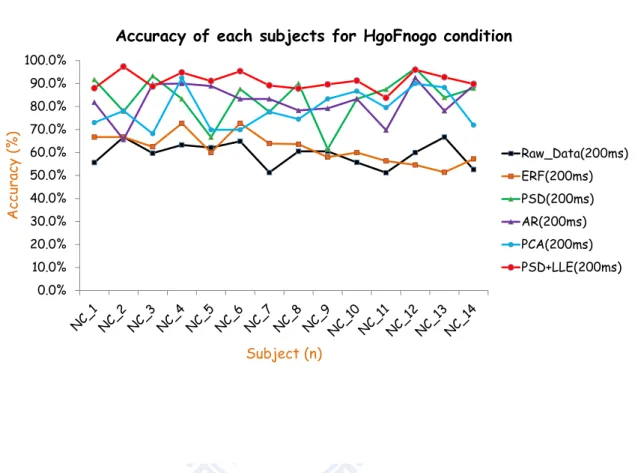
4.2 The recognition of each feature for each subject classification from HgoFnogo condition. . . 43
feature of both male and female subjects for FgoHnogo condition. . . 45
4.5 Summarized description of the classification performance obtained by each feature of both male and female subjects for HgoFnogo condition. . . 46
4.6 Classification accuracy for each feature averaged from the BD patients. . . 48
5.1 The experiments have eight different combinations. . . 51
5.2 We have only used four kinds of conditions to classify emotions. . . 52
5.3 The results of use of FgoOngo - Ongo as testing data. . . 53
5.4 The results of use of HgoOngo - Ongo as testing data. . . 54
5.5 The results of use of FgoOngo - Fgo as testing data. . . 55
5.6 The results of use of HgoOngo - Hgo as testing data. . . 56
5.7 The proportion of false-alarm and prediction for FgoHnogo condition. . . . 57
5.8 The proportion of false-alarm and prediction for HgoFnogo condition. . . . 58
5.9 The correlation between trials and accuracy for FgoHnogo condition. . . 61
5.10 The correlation between trials and accuracy for HgoFnogo condition. . . 62
List of Tables
3.1 Demographic data of all participant . . . 19
3.2 Four frequency bands with frequency range respectively . . . 26
3.3 The parameter set for each method . . . 31
4.1 The number of trials after EOG rejection for each subject. . . 38
4.2 The recognition accuracy of each feature for each subject classification for FgoHnogo condition. . . 40
4.3 The recognition accuracy of each feature for each subject classification for HgoFnogo condition. . . 41
4.4 Average each subject of each feature classification for FgoHnogo condition. 42 4.5 Average each subject of each feature classification for HgoFnogo condition. 43 4.6 The classification results by each feature of female subjects for FgoHnogo condition. . . 44
4.7 The classification results by each feature of male subjects for FgoHnogo condition. . . 45
4.8 The classification results of each feature of female subjects for HgoFnogo condition. . . 47
4.9 The classification results of each feature of male subjects for HgoFnogo condition. . . 47
4.10 Classification accuracy for each feature averaged from the BD patients for FgoHnogo condition. . . 47
4.11 Classification accuracy for each feature averaged from the BD patients for HgoFnogo condition. . . 48
5.1 The proportion of false-alarm and also prediction the wrong result for FgoHnogo condition . . . 59
5.2 The proportion of false-alarm and also prediction the wrong result for HgoFnogo condition . . . 60
5.3 The correlation between the number of trials and accuracy for FgoHnogo condition . . . 63
Chapter 1
Introduction
In this chapter we briefly introduce background knowledge of the thesis. In Section 1.1, we first briefly introduce the motivation of this study and survey the research works related to emotion recognition. Then Section 1.2 presents thesis scope. Finally Section 1.3 presents the thesis organization.
1.1
Motivation
What is emotion? Emotion is a complex physiological process and a psychological phenomenon. When a subject is exposed to physical or mental stimulation, the external stimulation will lead to all sorts of psychological reactions, which is called emotion. In our daily lives, emotions play a powerful and significant role in social network which can help people to understand others’ feelings. According to medical research findings, emo-tion is an important relaemo-tionship to the disorders in psychopathology, the survey based on the International Statistical Classification of Diseases and Related Health Problems 10th Revision (ICD-10) classification found this there are around 15% at population to suffering affective disorders [29]. Furthermore, affective disorder has been identified as century one of the three major diseases in the twenty-first. According to the World Health Organization survey (WHO) [29], affective disorders patients have been increasing, and resulting in se-rious social problems. Affective disorder is an accumulation of negative emotions in life. How to reduce the prevalence of depressive disorders is very important.
This is a very useful information for the application of intelligent environment from the emotion recognition. Recently construction and application of intelligent environments becomes a prosperous research field. The intelligent environment research aims to use information technology tools, that is to say, the application of intelligent environment re-search is to create a more friendly environment for real-world environment to increase perception and wisdom, the environment can take the initiative in service human. For ex-ample, when the system detection of negative emotions is increasingly from human, the system can timely adjust the environment temperature or light, because the comfortable environment that human positive emotion is increasingly.
ex-1.2 Thesis scope 3
pressions, voice and physiological signals. In the literature, there have been many research works which recognize emotions through external manifestation, such as facial expres-sions, voice and gestures, besides there can be observed the emotion expression, the signal also will often accompanied by physiological changes. In many of the emotion response, specific features of human facial expression, moreover often complex and diverse. We were to determine their expression via the change of facial features location. However, face de-tection and video were based on external manifestation, but not necessarily representative of their true inner feelings. In physiology, we realize that when emotional aroused, we cannot self-control of physiological response signal. Therefore, physiological signal is a very effective indicator.
Recognition the emotions from physiological signal can be achieved by several ways such as Electrocardiogram (ECG), Electromyogram (EMG), Blood volume pulse (BVP), Electrodermal activity (EDA, SC, GSR), Skin temperature (SKT), Respiration (RESP), Electroencephalography (EEG), and Magnetoencephalography (MEG), as shown in Figure 1.1.
The human physiology signals, modern medicine has confirmed that the brain’s various activities, including thoughts, emotions, desires and so on, the relationship between elec-trical current and chemical reactions of tend to come out, we can estimate use of the brain waveform. Therefore, in this study we propose an emotion recognition system based on brain signals.
1.2
Thesis scope
The objective of this thesis is to recognize emotion from the healthy by the MEG sig-nals. We preprocess the MEG signals and then extract feature, there are five kind of fea-tures. The first is the event-related magnetic fields (ERF) feature which extract from the latency and amplitude, the second is power spectral density (PSD) feature which extract from the power spectral density, the third is autoregressive (AR) model feature which ex-tract from the AR coefficients, the fourth is principal component analysis (PCA) feature which extract from the principal components, and the other one is locally linear embedding
EMG (Muscle tension)
BVP
(Blood volume pulse)
Respiration (Breathing rate) EEG/MEG (Brain waves) ECG (Heart rate) EDA/GSR/SC (Skin conductivity)
1.3 Thesis organization 5
(LLE), the feature of low dimensionality representation of dimensionality reduction from spatial. Finally, those features are used to differentiate the emotion by classification.
1.3
Thesis organization
In the following chapters, we will bring up the proposed methods, experiment results and some discussion in this work. The feature extract and classification procedure method will be introduced in Chapter 3, the classification results in Chapter 4. Then, we will have some discussion and conclusions in Chapter 5 and Chapter 6.
Chapter 2
Over the years, related to the study of the emotion recognition based on physiological signals, there have been many experts and scholars in the study, there are many methods have been proposed. The research about emotion recognition using physiological signals divided to two categories, autonomic nervous system and central nervous systems.
2.1
Emotion psychology
2.1.1
The definition of emotion
Daniel Goleman [4] defines the emotion as ”feeling, the idea of a specific, physiolog-ical state, psychologphysiolog-ical state, and related behavioral tendencies”. That is, the emotion consists of three parts: personal feelings, thoughts, and behavior, when the three parts are in equilibrium, is that mental health.
The general ways of emotion evoked by visual and auditory involve the same basic cir-cuit, both activated by the mirror neurons. The brain’s mirror neuron system observes how other people act to understand their intentions and then produces compassion. Neurosci-entists believe that the general observation and action system provides a neural mechanism which enable others’ to automatically understand others’ behavior, intentions and emo-tions. [20].
2.1.2
The theory of emotion
James-Lange theory of emotion
The American psychologist James (1884) and Lange (1885) was first proposed to ex-plain the emotion of psychologist. They believe that emotions are caused by physiological changes, rather than stimulation [10].
Event =⇒ arousal =⇒ interpretation=⇒ emotion
2.1 Emotion psychology 9
The American physiologist Cannon and his student Bard, they believe that cannot explain that only physiological responses to emotions, emotions and physiological changes should be simultaneously generated [3].
Event =⇒ simultaneous arousal and emotion
Schachter-Singer theory of emotion
Schachter-Singer theory of emotion is also called two-factor theory of emotion, because they believe that emotions are produced have two factors: (1) physiological responses, and (2) cognitive assessment [24].
Event =⇒ arousal=⇒ reasoning =⇒ emotion
2.1.3
The category of emotion
Before we proceed to the recognition of emotion, we must first understand how the classification of emotions, but there has not been consensus on the emotion classifica-tion, therefore, many researchers have put forward various regarding emotional classifi-cation. Although there are different categorization methods of emotions, but the emo-tion categories are basically the same. Some often refer to the emoemo-tion classificaemo-tion model as Plutchik’s [19] three-dimensional emotion model, as shown in Figure 2.1. Rus-sell’s [22] two-dimensional emotion mode, as shown in Figure 2.2, and Thayer’s [27] two-dimensional emotion mode, as shown in Figure 2.3.
In the Plutchik’s three-dimensional emotion mode, which the cones vertical dimen-sion represents intensity, and the circle represents degrees of similarity among the emo-tions [18]. The eight sectors are designed to indicate that there are eight primary emotion dimensions defined by the theory arranged as four pairs of opposites. In the exploded model the emotions in the blank spaces are the primary dyadsemotions that are mixtures of two of the primary emotions. The Russell’s two-dimensional emotion mode of affect with the horizontal axis representing the valence dimension and the vertical axis representing the arousal or activation dimension [25]. The Thayer’s two-dimensional emotion mode, which can be divided into four quadrants with four emotion [27].
Figure 2.1: Plutchik’s three-dimensional emotion mode [25].
2.2 Physiological signals 11
Figure 2.3: Thayer’s two-dimensional emotion mode [25].
In this study, we adopt 2-D model of the two emotion are fear and happy on behalf of positive and negative emotions and high arousal.
2.2
Physiological signals
2.2.1
Autonomic nervous system and peripheral nervous system
Emotion-specific activity in the autonomic nervous system was generated by construct-ing facial prototypes of emotion muscle by muscle and by relivconstruct-ing past emotional expe-riences. The autonomic activity produced distinguished not only between positive and negative emotions, but also among negative emotions [6].
Blood volume pulse (BVP)
BVP is a measurement of the blood flow, previous studies pointed out that human produce excitement, tension, anger, feel a stress and to greater emotional response , that will in-crease blood flow; but relaxed, calm, and sad, that will reduced blood flow. Therefore, the subjects’ emotion response is through changes in blood flow to detect, blood flow measured
usually by the fingertip.
Electrocardiogram (ECG)
ECG is a measurement of contractile activity of the heart. Previous studies pointed out that in a relaxed, happy, and calm state, heart rate will decrease; in the excitement, tension, and pressure state, heart rate will increase.
Electromyogram (EMG)
EMG is a measurement of muscle activity or frequency of muscle tension, previous studies pointed out that human in the tense state, the EMG rate will increase, but in the state of relaxation, EMG rate will decrease.
Respiration (RESP)
RESP is a measurement of the frequency to breathing, when the lungs inhale air to make the chest expand; the exhalation of air, chest compressed air by discharges, chest will be-come smaller. The breathing is the same as heart rate, that have a regular cycle, so the change through the respiratory rate, can be observed emotional changes of subjects as well. Previous studies pointed out that human be excited, nervous, and angry, the breathing rate will increase; be relaxed, calm, pleasant, the breathing rate will decrease.
Skin conductivity (SC, GSR, or EDA)
EDA is a measurement of the skin ability to conduct electricity. Previous studies pointed out that skin conductivity and the degree of emotional arousal are linearly related. The emotion generates by induced while, that will to enhance the effect of the sympathetic ner-vous, so the surface of the skin secretion of sweat glands, skin humidity changes, increase in the subject’s skin conductivity, cause dramatic changes in GSR signals. Therefore, when people the tension, excitement, and fear, the skin conductivity higher.
2.2 Physiological signals 13
Figure 2.4: Kim, K. H et al. development of emotion recognition system [13].
Kim et al., [13]experimented with emotion recognition. Kim, K. H. using voice, video and picture as stimuli to induce four emotions. The four emotions are sadness, anger, stress, and surprise emotions. They using three physiological signals are collected: ECG, EDA, and SKT, will be to collect the physiological signals of the feature extraction, and using support vector machine for classification of the data, as shown in Figure 2.4.
Andre et al., [12], research and development of a scheme of emotion recognition. The experiment the main stimulus is music, using music to stimulate the subjects of real emo-tional state. The use of four-channel physiological signal sensors (biosensors): ECG, EMG, SC, and RSP respectively. Using an extended linear discriminant analysis (pLDA) classi-fied four kinds of musical emotions: positive/high arousal, negative/high arousal, nega-tive/low arousal, and posinega-tive/low arousal, as shown in Figure 2.5. The recognition accu-racy was 95% and 70% for subject-dependent and subject-independent classification
Figure 2.5: Kim, J. and Andre, E. development of supervised statistical classification sys-tem for emotion recognition [12]
2.2.2
Central nervous system
In addition to periphery biosignals, signals captured from the brain in central nervous system (CNS) have been proved to provide informative characteristics in responses to the emotional states. CNS has been used in cognitive neuroscience to investigate the regulation and processing of emotion for the past decades [2] [5]. The related references indicate that the visual processing in the brain is within 100ms followed by 100ms of emotion processing. After 200ms there can be behavior phenomenon involved in the neuron network activities. [1] [17] [26].
Power spectra of the EEG were often assessed in several distinct frequency bands, such as delta (δ : 1 − 3Hz), theta (θ : 4 − 7Hz), alpha (α : 8 − 13Hz), beta (β : 14 − 30Hz), and gamma (γ : 31 − 50Hz), to examine their relationship with the emotion states [9] [15] [16].
Magnetoencephalography (MEG)
MEG is a measurement of magnetic fields produced by the ensemble of neuronal activities inside brain.
Electroencephalography (EEG)
2.3 Feature extraction 15
Figure 2.6: The 2-D emotional space [14].
Frantzidis et al., [7] proposes a methodology use for EEG signals for emotion recogni-tion, the system the main stimulus is IAPS collection in which picture, classification of four emotional states HVHA (high valence and highly arousal), HVLA (high valence and low arousal), LVHA (low valence and highly arousal), LVLA (low valence and low arousal) is performed by a Cartesian 2-D emotional space, as depicted in Figure 2.6. The achieved overall classification rates were 79.5% and 81.3 % for the MD and SVM.
Jung et al., [11] proposes EEG-based emotion recognition system, the system the main stimulus is music, use music to stimulate the subjects emotional, classification of four emotional states: joy, anger, sadness, and pleasure, and obtained an averaged classification accuracy of 82.29% ± 3.06%.
2.3
Feature extraction
In research on brain wave about emotion recognition, researchers majority using feature extraction methods. The detection of the characteristic waveform use event-related poten-tial and spectral power changes, extraction of useful information feature for classification. The event-related potential was averaged ERPs extracted from each channels, therefore,
amplitude and latency feature were extracted for the P100, N100, P200, N200, and P300 [7].
The power spectra were calculated using short-time Fourier transform (STFT) or fast Fourier transform (FFT), the resultant spectral time series was averaged into five frequency bands, delta (δ : 1 − 3Hz), theta (θ : 4 − 7Hz), alpha (α : 8 − 13Hz), beta (β : 14 − 30Hz), and gamma (γ : 31 − 50Hz). The frequency and the corresponding with energy and the corresponding were used as features in the classification [7] [28] [9].
Chapter 3
Classification of affective evoked brain
activities
Stimulus MEG recording Preprocessing Feature extraction and feature selection Classification
Fear
Figure 3.1: Framework of this thesis.
In this chapter, we describe the experiment procedure. We first introduce the materials used in the experiment, and then introduce the methods of experiment, which can be split into three main steps: (1) feature extraction, (2) feature selection, and (3) classification.
The emotion recognition system as shown in Figure 3.1. In this study, the system can be divided into five parts: signal acquisition, signal pre-processing, feature extraction, feature selection, and classification. In addition to frequency domain analysis, we also used to retrieve from the MEG waveform feature, predictive model to assess, linear dimension reduction, as well as non-linear dimension reduction to extract features, hoping to find the most representative and really to represent the emotional feature.
3.1 Materials 19
3.1
Materials
3.1.1
Participants
In this work, participants were 14 healthy (9 females and 5 males; ages between 30-55 years, mean 39.43 ± 9.02 years), and 14 bipolar disorder (BD) patients (11 females and 3 males; ages between 25-62 years, mean 41.71 ± 10.62 years), all right-handed. Experimen-tal design and data collection were performed by Taipei Veterans General HospiExperimen-tal. The main contribution of this study is the analysis of the MEG signals. Demographic data of all participant as shown in Table 3.1.
Table 3.1: Demographic data of all participant.
Normal (NC) Bipolar Disorder(BD)
Participant, n 14 14
Gender (male/female), n 5/9 3/11
Age (mean age), mean SD 39.43±9.02 41.71 ±10.62
Handedness (right), n 14 14
3.1.2
Experimental paradigm
Affective visual stimuli consist of face images with two different emotions which are fear and happy. In this experiment, the participants are placed in a magnetic shielded room and are presented with the visual stimuli, and the brainwave signals induced by the stimuli are recorded by the MEG device. The task is to confirm that the participants can correctly recognize the emotion expressed. Participants can press the button while recognizing the presented face image is fear or happy. Each stimulus is displayed for 700 ms, and then a
Time
Pictures of emotional stimuli (700 ms)
Fixation cross (1850~2150 ms)
One epoch
Figure 3.2: The experiment paradigm of emotion recognition.
fixation cross appears for a random time length ranging from 1850 ms to 2150 ms. The whole experiment paradigm is shown in Figure 3.2.
3.1.3
MEG device
MEG system is used for recording of the minute magnetic field generated by human brains electrical activity within the living human brain. The measurement was acquired by a whole-head 306-channel Neuromag Vectorview system (Elekta Neuromag Vectorview, Finland) which located inside a magnetically shielded room (Euroshield, Eura, Finland) at Integrated Brain Research Unit of Taipei Veterans General Hospital. The MEG system has 306 channels contains 102 magnetometers, 204 planar gradiometers 24 bits analog to digital conversion and up-to-8 kHz sampling rate which is sufficient to probe the fast variation inside human brain. The MEG device is shown in Figure 3.3.
3.1 Materials 21
3.1.4
Neurophysiological recordings
MEG signal were recorded by a whole-head 306-channel Neuromag Vectorview system which located inside a magnetically shielded room at Integrated Brain Research Unit of Taipei Veterans General Hospital. The signals were recorded participants emotion state. The sampling rate was set at 1001.6 Hz and band-pass filtered was 0.03-330 Hz.
3.1.5
Data preprocessing
The brain signal relative to environmental interference noises is comparatively small. Hence we were to enhance the signal-to-noise ratio (SNR). The MEG signals were offline preprocessed as shown in Figure 3.4: (1) eliminate bad channels which has abnormal record, (2) the rejection of ocular artifact-contaminated trials, leaving only the segments without ocular artifacts-contaminated trials to accepted for further analysis, (3) signal space projection (SSP) was exploited to eliminate the unbalanced noise effect, (4) we use band-pass filter to exclude those unavoidable artifacts, and the signals were hardware band-band-pass filtering between 2 and 35 Hz, (5) we conduct the baseline correction by subtracting a baseline from the recordings. The baseline is usually estimated by the mean of in the 300 ms prior to stimulus, at which it the recordings are unaffected by the stimulus.
3.2
Feature extraction (feature generation)
3.2.1
Event-related magnetic fields
Event-related magnetic fields (ERF) is a measurement of neuronal activity patterns as-sociated with the perceptual and cognitive processes occurring in the brain response to stimuli, that evoke a specific waveforms by the peak amplitude and latency.
We used ERF analysis of MEG recordings of emotion with fear and happy, stimuli is based on FgoHnogo and HgoFnogo tasks. The 200 ms for each participant, channels and emotion states, and each component is according to its latency and amplitude as shown in Figure 3.5, 3.6. Therefore, amplitude and latency feature are extracted for ERF compo-nents.
3.2 Feature extraction (feature generation) 23
Bad-channel elimination
EOG
rejection SSP Bandpass filte correction Baseline Bad-channel elimination EOG rejection SSP Recording
0 20 40 60 80 100 120 140 160 180 200 -4 -3 -2 -1 0 1 2 3 4 5 6x 10 -12 Time [ms] A m p li tu d e [ fT /c m ] FgoHnogo Happy Fear
3.2 Feature extraction (feature generation) 25 0 20 40 60 80 100 120 140 160 180 200 -4 -3 -2 -1 0 1 2 3 4 5x 10 -12 Time [ms] A m p li tu d e [ fT /c m ] HgoFnogo Frar Happy
3.2.2
Power spectral density
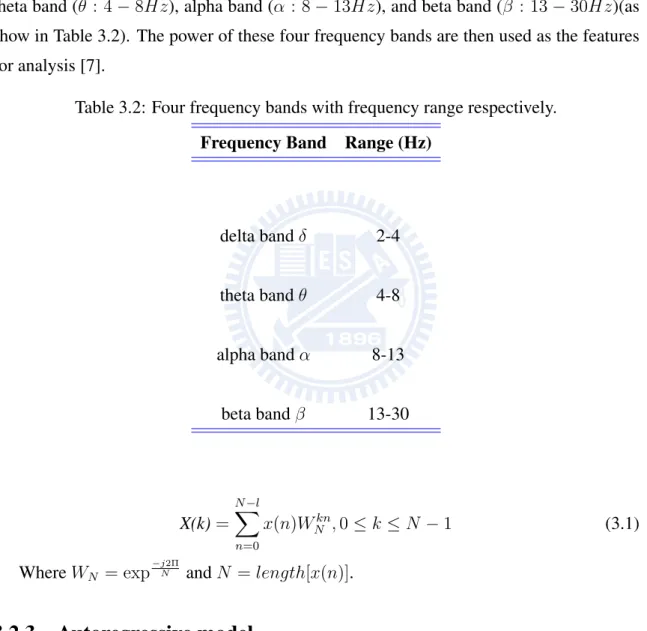
Powers of different frequency bands are one of the most commonly used features in the frequency domain analysis. First, MEG signals are transformed from time domain to frequency domain using fast Fourier transform (FFT) method. The spectrum of MEG signals is then further divided into four frequency bands, which are delta band (δ : 2−4Hz), theta band (θ : 4 − 8Hz), alpha band (α : 8 − 13Hz), and beta band (β : 13 − 30Hz)(as show in Table 3.2). The power of these four frequency bands are then used as the features for analysis [7].
Table 3.2: Four frequency bands with frequency range respectively.
Frequency Band Range (Hz)
delta band δ 2-4 theta band θ 4-8 alpha band α 8-13 beta band β 13-30 X(k)= N −l X n=0 x(n)WNkn, 0 ≤ k ≤ N − 1 (3.1) Where WN = exp −j2Π N and N = length[x(n)].
3.2.3
Autoregressive model
Autoregressive (AR) model is one of the common linear forecasting model, the model prediction the data in the next time interval is based on the correlation between the variables and time series. It is commonly used in filed statistics and signal processing.
3.2 Feature extraction (feature generation) 27
The AR model is defined by the equation:
xi(t) =
p
X
n=1
ai(n)xi(t − n) + εi(t), n = 1, 2, ..., p (3.2)
The observed MEG signal can be written as by xi(t), i = 1, 2, .., n, t = 1, 2, ..., T,
where i is the index of the MEG channels and t is the time point, p is the model order, ai(n)
is the AR model coefficients, xi(t − n) is the data before time t, and εi(t) denotes the noise.
3.2.4
Principal component analysis
Principal Component Analysis (PCA) is one of the common methods for feature extrac-tion and dimensionality reducextrac-tion. The PCA objective is to reduce high dimensional data set so we can use less number of interrelated variables and retaining as possible as much of variations in data set. Generally, high-dimensional data will consume more time to perform computing or classifying, therefore PCA method is to do a group of dimension reduction, and use fewer low dimensional data to represent a large group of data. In this research, we used PCA to reduce the MEG temporal signals as feature. Through PCA method, we can easily project the MEG temporal signals from 200-dimension to lower dimension space. The steps of PCA method are as following:
Step 1: Calculate the mean vectors
m= 1 nT r nT r X i=1 xi (3.3)
Where xi = [x1, x2, ..., xn]|is n − dimensionality MEG signals training data, nT r is
number of the training data.
Step 2: Calculate the scatter matrix of the feature vectors
S= nT r X i=1 (xi− m)(xi− m)|= xx| (3.4) Where S is n ∗ n matrix.
e|Se = λ (3.5) Step 4: Calculate the projected feature vectors (principal components)
yi = A|(xi − m), whereA = [e1, e2, ..., ed] (3.6)
Where A is n ∗ d matrix, consist of the eigenvectors, yi = [y1, y2, ..., yd]| is the PCA
feature vectors.
3.2.5
Locally linear embedding
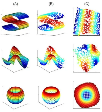
The problem of dimensionality reduction applications in many fields of machine learn-ing, pattern recognition, data compression, and neural computation etc. Here we describe Locally Linear Embedding (LLE), LLE is a nonlinear dimension reduction method that it can project high dimensional data to a lower-dimensional manifold. In the dimension reduction process, every point will retain the relationship with the original point, these neighboring points will not change with any displacement or rotation as illustrated in Fig-ure 3.7.
The LLE algorithm there are three main steps as shown in Figure 3.8. The algorithm is summarized in the following three steps [8]:
Step 1: For each pointxi = 1, 2, , n, search for its nearest neighbors.
Step 2: Compute the weightsW (i, j), i, j = 1, 2, n, the best reconstruct each point xi ,
from its nearest neighbors, so that to minimize the cost.
ε(W ) = n X i=1 k xi− n X j=1 W (i, j)xij k2 (3.7)
Where, xij is the jth neighbor of the ith point. The weights cost function to satisfy two
constraints: (1) Only can used the neighbor at each point xi to reconstructed, W (i.j) = 0,
if xj does not neighbors of xi.
n
X
j=1
3.2 Feature extraction (feature generation) 29
Figure 3.7: The example of nonlinear dimensionality reduction as illustrated for data (B) sampled from a two dimensional manifold (A). By way of nonlinear dimensionality reduc-tion algorithm (LLE), the data is mapped to two-dimensional space (C) [23].
3.3 Selected features 31
Step 3: Use the weights previous step to compute the corresponding points yi, i =
1, 2, , n, so that to minimize the cost function to find a new d-dimensional coordinates yi.
Φ(y) = n X i=1 k yi− X j W (i, j)yj k2 (3.9)
Summing up the above five methods at parameter set. The parameter set for each method as shown in Table 3.3.
Table 3.3: The parameter set for each method.
Methods parameter set
AR model 15
PCA Number of sorted eigenvalues with 95% of accumulated values
LLE 20
3.3
Selected features
The goal of feature selection is to select the most influential features from the original feature that recognition rates can reach the maximum value. Through the process of feature selection, we can achieve accuracy.
We select the features PSD that have the highest recognition rate to be combined with LLE. Use PSD method to extract temporal information and then use LLE method to extract spatial features..
w
Class A
Class B
Support vector
Figure 3.9: SVM classifier. There are two different data and we need to find a decision boundary to separate two classes of data and the margin between the two is maximal.
3.4
Classification
3.4.1
Support vector machine
In this work, we use support vector machine (SVM) to classify the emotion state for each MEG segment.
SVM is a statistical-based theory which is supervised learning method used for classi-fication and regression analysis. In recent years, it has been widely used in pattern recogni-tion and data classificarecogni-tion. Also because of its high accuracy and great ability to deal with a large number of predictors, it often use in biomedical.
The main idea of SVM is to determine a hyperplane which can separate different classes from all samples, and allow maximal margins between the training data and de-cision boundary as shown in Figure 3.9 illustrate the classifier of SVM.
3.4 Classification 33
from all data. Assume there is a space data Rd, it has N different classes of sample. Then
the new samples near N in training set can be more easy to classified correctly. Given the training data x and y, it can seeks the optimal solution.
The linear discriminant function is g(x) = wTx + w0, and then the distance between
sample x and the decision boundary (g(x) = 0) is given by
|wTx + w
0|
kwk . (3.10)
Scaling Wand w0 by a positive constant does not change the boundary, to make the
values of Wand wounique, we add the requirement to support vectors:
|wTx + w
0| = 1. (3.11)
This distance from support vctors to the largest margin hyperplane is 1/||w||, margin is given by 2/||w||, and the maximizing the margin is the same as minimizing ||w||. we can phrase the task of finding the decision boundary in SVM as an optimization problem:
To minimize
J = 1
2kwk
2
(3.12) The objective of SVM is to maximize the margin 2/||w||
(
wTx
i+ w0 ≥ 1
wTxi+ w0 ≤ −1.
(3.13)
subject to the constraints yi(wTxi+ w0) ≥ 1, ∀i
Here yi = +1, ∀xi ∈ ω1 yi = +1, ∀xi ∈ ω2. (3.14)
Using Lagrange multipliers to include the constraints:
Ł = 1 2kwk 2 − N X i=1 λi[yi(w|xi+ w0) − 1], (3.15)
w = N X i=1 λiyixi and N X i=1 λiyi = 0. (3.16)
These are the solutions for minimizing J with the constraints. The problem now is to determine the Lagrange multipliers. Once the optimal Lagrange Multipliers are obtained through some optimization procedure, we can compute w using
w =
N
X
i=1
λiyixi. (3.17)
The value w0 can be computed using wo= y−1i − wTxi, where xi is a support vector.
Using the same techniques of the linearly separable cases, we end up with a very similar optimization problem: to maximize
Ł = N X i=1 λi− 1 2 N X i=1 N X j=1 λiλjyiyjx|ixj, (3.18)
subject to the constraints
N
X
i=1
λiyi = 0 andλi > 0, ∀i (3.19)
L is a concave function with respect to λ
The optimization task, with x now mapped to high-dimensional space, becomes the maximization of L = N X i=1 λi − 1 2 N X i=1 N X j=1 λiλjyiyj[Φ(xi|Φ(xj)] = N X i=1 N X j=1 λiλjyiyjK(xi, xj)(3.20)
Subject to the constraints
N
X
i=1
= 0 and 0 ≤ λi ≤ C, ∀i (3.21)
We define the kernel function K(xi, xj) = Φ(xi)|Φ(xj)
Different common types of K(xi, xj) :
3.4 Classification 35
2. Polynomial: K(xi, xj) = (gxiT xj + g)d, g > 0 :
3. Radial basis function (RBF): K(xi, xj) = exp−
gkxi−xj k2
2σ2 )
Where σ is specified by the user and common to all kernels.
3.4.2
Evaluation
It is the most common evaluative method through k-fold cross validation.
The data sample is randomly partitioned divided into k samples, a separate sub-samples is retained as validation data for testing the model, other K-1 sub-sub-samples used for training. Repeated k times to model the work, the k results from the folds then can be averaged to produce a single estimation. In this study, the model evaluation we use 10-fold cross-validation.
1 0~200 ms MEG data 204 channels ERF PSD AR model PCA LLE Latency Amplitudes δ, θ, α, β Coefficients Principal components Low-dimensional representation Classifier Waveform Frequency analysis Parametric Temporal feature Spatial feature 204×2 204×order 204×#(95% eigenvalues) 4×15
Selected feature
Feature extraction (feature generation)
Chapter 4
In this study, we show the recognition accuracy of the each participant in each of the feature. And then show the recognition accuracy for the discrepancy between normal sub-jects and BD patients.
4.1
Preprocessing results
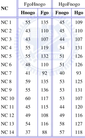
For each condition, there are two combinations of tasks: Go-140 trials and Nogo-60 trials from total 200 trials. In Table 4.1. We preprocessed the number of trials after EOG rejection for each subject.
Table 4.1: The number of trials after EOG rejection for each subject.
NC FgoHnogo HgoFnogo Hnogo Fgo Fnogo Hgo
NC 1 55 135 45 109 NC 2 43 110 45 110 NC 3 43 107 44 107 NC 4 55 119 54 131 NC 5 55 132 51 126 NC 6 48 110 51 126 NC 7 41 92 40 93 NC 8 59 135 53 125 NC 9 55 136 53 131 NC 10 60 117 53 107 NC 11 45 115 44 120 NC 12 49 108 49 116 NC 13 54 116 58 127 NC 14 37 88 57 118
4.2 Results of all participants 39
4.2
Results of all participants
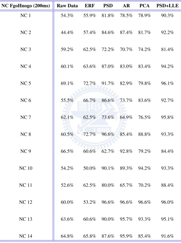
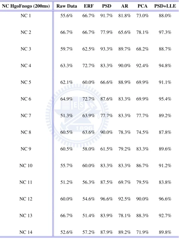
We were collecting 14 participants for brain signals through the artifact removal and filter, feature extraction, and then use ten-fold cross validation method to proceed SVM classification of recognition rate, calculated each participant recognition rate and an av-erage of all the participants recognition rate, the results shown in the Table 4.2, 4.3, and Figure 4.1 4.2.
The recognition accuracy results of each subject for PSD combine LLE feature ex-traction is highest recognition accuracy of 96.1% and 97.3% for FgoHnogo condition and HgoFnogo condition classification, respectively, as seen in Table 4.2, 4.3.
The recognition accuracy results of each subject for FgoHnogo condition and HgoFnogo condition classification, respectively as shown in Figure 4.1, 4.2.
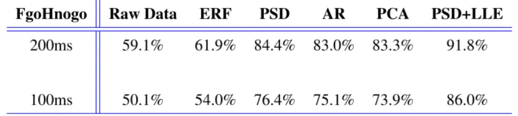
Can be found from Table 4.4, 4.5, 4.3, used with the success of PSD combine LLE feature can recognition two categories of happy and fear emotion from brain signal, and get 91.8% and 91.1% of the high rate of recognition results.
4.3
Results of gender difference participants
In Table 4.6, 4.7, and Figure 4.4, the recognition accuracy of between female and male subjects for the FgoHnogo condition classification. The recognition accuracy was clearly better use the feature selection from PSD combine LLE, recognition accuracy performance of 91.2% and 91.3% for female and male, respectively.
The recognition accuracy of between female and male subjects for the HgoFnogo con-dition classification. Accuracy was clearly better using the feature extraction from PSD combine LLE of female and male, HgoFnogo condition accuracy performance of 92.9% and 90.7%, as shown in Table 4.8, 4.9, and Figure 4.5.
4.4
Results of BD patients
We were collecting 14 BD patients for brain signals through the artifact removal and filter, feature extraction, and then use ten-fold cross validation method to proceed SVM
Table 4.2: The recognition accuracy of each feature for each subject classification for FgoHnogo condition.
NC FgoHnogo (200ms) Raw Data ERF PSD AR PCA PSD+LLE NC 1 54.3% 55.9% 81.8% 78.5% 78.9% 90.3% NC 2 44.4% 57.4% 84.6% 87.4% 81.7% 92.2% NC 3 59.2% 62.5% 72.2% 70.7% 74.2% 81.4% NC 4 60.1% 63.6% 87.0% 83.0% 83.4% 94.2% NC 5 69.1% 72.7% 91.7% 82.9% 79.8% 96.1% NC 6 55.5% 66.7% 86.6% 73.7% 83.6% 92.7% NC 7 62.1% 62.5% 73.6% 64.9% 76.5% 95.8% NC 8 60.5% 72.7% 96.6% 85.4% 88.8% 93.3% NC 9 66.5% 60.6% 62.7% 92.8% 79.2% 84.4% NC 10 54.2% 50.0% 90.1% 89.3% 94.2% 93.3% NC 11 52.6% 62.5% 80.0% 65.7% 70.2% 88.4% NC 12 60.0% 53.2% 96.6% 96.6% 96.6% 96.0% NC 13 63.6% 60.6% 90.0% 95.7% 93.3% 95.1% NC 14 64.8% 65.8% 87.6% 95.9% 85.4% 91.6%
4.4 Results of BD patients 41
Table 4.3: The recognition accuracy of each feature for each subject classification for HgoFnogo condition.
NC HgoFnogo (200ms) Raw Data ERF PSD AR PCA PSD+LLE NC 1 55.6% 66.7% 91.7% 81.8% 73.0% 88.0% NC 2 66.7% 66.7% 77.9% 65.6% 78.1% 97.3% NC 3 59.7% 62.5% 93.3% 89.7% 68.2% 88.7% NC 4 63.3% 72.7% 83.3% 90.0% 92.4% 94.8% NC 5 62.1% 60.0% 66.6% 88.9% 69.9% 91.1% NC 6 64.9% 72.7% 87.6% 83.3% 69.9% 95.4% NC 7 51.3% 63.9% 77.7% 83.3% 77.7% 89.2% NC 8 60.5% 63.6% 90.0% 78.3% 74.5% 87.8% NC 9 60.5% 58.0% 61.5% 79.2% 83.3% 89.6% NC 10 55.7% 60.0% 83.3% 83.3% 86.7% 91.2% NC 11 51.2% 56.3% 87.5% 69.7% 79.5% 83.8% NC 12 60.0% 54.6% 96.6% 92.5% 90.0% 96.6% NC 13 66.7% 51.4% 83.9% 78.1% 88.3% 92.7% NC 14 52.6% 57.2% 87.9% 89.2% 71.9% 89.8%
0.0% 10.0% 20.0% 30.0% 40.0% 50.0% 60.0% 70.0% 80.0% 90.0% 100.0% Ac cu racy (%) Subject
Accuracy of each subjects for FgoHnogo condition
Raw_Data(200ms) ERF(200ms) PSD(200ms) AR(200ms) PCA(200ms) PSD+LLE(200ms)
Figure 4.1: The recognition of each feature for each subject classification from FgoHnogo condition.
Table 4.4: Average each subject of each feature classification for FgoHnogo condition.
FgoHnogo Raw Data ERF PSD AR PCA PSD+LLE 200ms 59.1% 61.9% 84.4% 83.0% 83.3% 91.8%
4.4 Results of BD patients 43 0.0% 10.0% 20.0% 30.0% 40.0% 50.0% 60.0% 70.0% 80.0% 90.0% 100.0% Ac cu racy (%) Subject (n)
Accuracy of each subjects for HgoFnogo condition
Raw_Data(200ms) ERF(200ms) PSD(200ms) AR(200ms) PCA(200ms) PSD+LLE(200ms)
Figure 4.2: The recognition of each feature for each subject classification from HgoFnogo condition.
Table 4.5: Average each subject of each feature classification for HgoFnogo condition.
HgoFnogo Raw Data ERF PSD AR PCA PSD+LLE 200ms 59.3% 61.9% 83.5% 82.4% 78.8% 91.1%
0.0% 10.0% 20.0% 30.0% 40.0% 50.0% 60.0% 70.0% 80.0% 90.0% 100.0% A ccuracy (%) Feature
HgoFnogo (All normal subjects)
200ms 100ms 0.0% 10.0% 20.0% 30.0% 40.0% 50.0% 60.0% 70.0% 80.0% 90.0% 100.0% A ccuracy (%) Feature
FgoHnogo (All normal subjects)
200ms 100ms
Figure 4.3: Average each subject of each feature classification.
Table 4.6: The classification results by each feature of female subjects for FgoHnogo condition.
FgoHnogo Raw Data ERF PSD AR PCA PSD+LLE 200ms 59.1% 63.8% 81.9% 79.9% 80.7% 91.2%
4.4 Results of BD patients 45
Table 4.7: The classification results by each feature of male subjects for FgoHnogo condition.
FgoHnogo Raw Data ERF PSD AR PCA PSD+LLE 200ms 59.0% 58.4% 88.9% 88.6% 87.9% 91.3% 100ms 49.8% 47.5% 69.8% 72.5% 71.8% 85.5% 0.0% 10.0% 20.0% 30.0% 40.0% 50.0% 60.0% 70.0% 80.0% 90.0% 100.0% A ccuracy (%) Feature
FgoHnogo (Female normal subjects)
200ms 100ms 0.0% 10.0% 20.0% 30.0% 40.0% 50.0% 60.0% 70.0% 80.0% 90.0% 100.0% A ccuracy (%) Feature
FgoHnogo (Male normal subjects)
200ms 100ms
Figure 4.4: Summarized description of the classification performance obtained by each feature of both male and female subjects for FgoHnogo condition.
0.0% 10.0% 20.0% 30.0% 40.0% 50.0% 60.0% 70.0% 80.0% 90.0% 100.0% A ccuracy (%) Feature
HgoFnogo (Male normal subjects)
200ms 100ms 0.0% 10.0% 20.0% 30.0% 40.0% 50.0% 60.0% 70.0% 80.0% 90.0% 100.0% A ccuracy (%) Feature
HgoFnogo (Female normal subjects)
200ms 100ms
Figure 4.5: Summarized description of the classification performance obtained by each feature of both male and female subjects for HgoFnogo condition.
4.4 Results of BD patients 47
Table 4.8: The classification results of each feature of female subjects for HgoFnogo condition.
FgoHnogo Raw Data ERF PSD AR PCA PSD+LLE 200ms 60.5% 65.2% 81.1% 82.2% 76.3% 92.9%
100ms 54.7% 55.7% 80.2% 79.4% 74.1% 87.1%
Table 4.9: The classification results of each feature of male subjects for HgoFnogo condition.
FgoHnogo Raw Data ERF PSD AR PCA PSD+LLE 200ms 57.2% 55.9% 87.8% 82.6% 83.3% 90.7%
100ms 49.8% 51.6% 83.3% 75.5% 74.3% 86.6%
classification of recognition rate, calculated each participant recognition rate and an aver-age of all the participants recognition rate, the results shown in the Table 4.10, 4.11, and Figure 4.6. The BD patients recognition accuracy is only 77.0%, the result is worse to compare NC, even though it is selected better feature.
Table 4.10: Classification accuracy for each feature averaged from the BD patients for FgoHnogo condition.
FgoHnogo Raw Data ERF PSD AR PCA PSD+LLE 200ms 30.7% 46.9% 68.9% 65.4% 62.2% 77.0%
Table 4.11: Classification accuracy for each feature averaged from the BD patients for HgoFnogo condition.
HgoFnogo Raw Data ERF PSD AR PCA PSD+LLE 200ms 44.4% 44.8% 68.9% 58.9% 59.6% 72.3% 100ms 42.3% 47.1% 58.5% 58.3% 51.2% 64.2% 0.0% 10.0% 20.0% 30.0% 40.0% 50.0% 60.0% 70.0% 80.0% 90.0% 100.0% A ccuracy (%) Feature FgoHnogo (BD patients ) 200ms 100ms 0.0% 10.0% 20.0% 30.0% 40.0% 50.0% 60.0% 70.0% 80.0% 90.0% 100.0% A ccuracy (%) Feature HgoFnogo (BD patients) 200ms 100ms
Chapter 5
Discussion
From this study experimental results, several research questions will be discussion as follows: (1) Classification using emotions or conditions? (2) Behavioural results, and (3) Effects of on the number of trials accuracy.
5.1
Classification using emotions or conditions?
Our experiments have eight different combinations of conditions and task: (1) FgoHnogo - Hnogo (2) FgoHnogo - Fgo (3) HgoFnogo - Fnogo (4) HgoFnogo - Hgo (5) FgoOnogo - Onogo (6) FgoOnogo - Fgo (7) HgoOnogo - Onogo (8) HgoOnogo - Hgo, as shown in Figure 5.1, however, in this study, we have only used four kinds of conditions to classify emotions, as shown in Figure 5.2. In order to determine whether to recognize the difference conditions, therefore, we have to test: use the FgoHnogo Fgo and HgoFnogo -Hgo as training data and the FgoHnogo - Hnogo as test data, from the testing recognition results, we can see the testing data will be classified into HgoHnogo - Hgo with accuracy 4.4% (one subject), 6.0% (one subject), and 0% (other subjects).
Then we use the task to have nothing to do with emotion to verify, first using FgoOnogo - Fgo and HgoOnogo - Hgo as testing data, respectively. We found the testing data will be classified into FgoHnogo - Fgo with accuracy 63.0% (one subject), 90.7% (one subject), and 100% (other subjects) of FgoOnogo - Fgo, and HgoOngo - Hgo will be classified into HgoFngo - Hgo with accuracy 57.0% (one subject), 87.0% (one subject), and 100% (other subjects), as shown in Figure 5.5, 5.6. Finally, we using FgoOnogo - Ongo and HgoOnogo - Ongo as testing data, respectively, as shown in Figure 5.3, 5.4, the results found it will be accompanied by conditions in which the effects of the emotion pictures, we can get that will be affected by different conditions. Therefore, we must distinguish the different conditions of individual recognition.
5.2
Behavioural results
In this study, we use Go and Nogo task to verify the subject’s emotions, because each subject’s different viewpoint on the emotion, we use the Go and Nogo task of false-alarm
5.2 Behavioural results 51
FgoHnogo
HgoFnogo
FgoOnogo
HgoOnogo
Hnogo Fnogo Onogo Onogo Fgo Hgo Fgo Hgo No Fear Fear Happy Happy Fear No Happyconditions
tasks
emotions
FgoHnogo
HgoFnogo
Hnogo Fnogo Fgo Hgo Fear Fear Happy Happyconditions
tasks
emotions
5.2 Behavioural results 53 FgoHnogo - Fgo HgoHnogo - Hgo FgoOnogo - Ongo Training data Testing data 92.25%, 91.07%, 88.37%, 91.54%, 100%, 84.75%, 96.39%, 88.53%, 84.10%, 88%, 93.06%, 83.25%, 69.29%, 84.71%
FgoHnogo - Fgo HgoHnogo - Hgo HgoOnogo - Ongo Training data Testing data 77.19%, 92.64%, 100%, 84.62%, 99.15%, 84.14%, 93.48%, 88.91%, 88.73%, 75%, 91.13%, 89.23%, 94.44%, 92.30%
5.2 Behavioural results 55 FgoHnogo - Fgo HgoHnogo - Hgo FgoOnogo - Fgo Training data Testing data One subject: 63.0 % One subject: 90.7 % Other subjects: 100 %
FgoHnogo - Fgo HgoHnogo - Hgo HgoOnogo - Hgo Training data Testing data One subject: 57.0 % One subject: 87.0 % Other subjects: 100 %
5.3 Effects of on the number of trials accuracy 57
Figure 5.7: The proportion of false-alarm and prediction for FgoHnogo condition.
the results with the results of also prediction the wrong, to explore whether there is any relationship between false-alarm and also prediction the wrong result. This can be seen in Figure 5.7, 5.8, the false-alarm corresponds to also prediction the wrong result is not a trend. The analysis was conducted of the data in Table 5.1, 5.2, and from the results of that analysis, this proportion is 19% and 13%, therefore, the false-alarm and also prediction the wrong result is not relevant.
5.3
Effects of on the number of trials accuracy
In this study, there are 200 trials combinations of each condition, due to recorded MEG signals are usually contaminated with noises, the preprocessing procedure is before the feature extract, we were remove EOG interference, the removal of EOG will also remove some of useful information of signals. When the subjects were rejected a lot of EOG, this is not a good measurement situation, therefore, we want to explore, whether a correlation
5.3 Effects of on the number of trials accuracy 59
Table 5.1: The proportion of false-alarm and also prediction the wrong result for FgoHnogo condition.
FgoHnogo False-alarm Prediction
NC 1 2 0 NC 2 2 0 NC 3 2 0 NC 4 2 0 NC 5 2 0 NC 6 2 0 NC 7 3 1 NC 8 3 1 NC 9 5 2 NC 10 5 1 NC 11 6 2 NC 12 6 2 NC 13 6 0 NC 14 16 3 total 62 12 proportion 19%
Table 5.2: The proportion of false-alarm and also prediction the wrong result for HgoFnogo condition.
HgoFnogo False-alarm Prediction
NC 1 0 0 NC 2 0 0 NC 3 0 0 NC 4 1 0 NC 5 1 0 NC 6 1 0 NC 7 2 0 NC 8 2 0 NC 9 3 0 NC 10 4 0 NC 11 5 1 NC 12 5 2 NC 13 5 0 NC 14 9 2 total 38 5 proportion 13%
5.3 Effects of on the number of trials accuracy 61 50.0% 60.0% 70.0% 80.0% 90.0% 100.0% 37 41 43 43 45 48 49 54 55 55 55 55 59 60 A ccuracy (%) Trial (n) FgoHnogo
Figure 5.9: The correlation between trials and accuracy for FgoHnogo condition.
exists between the number of trials and accuracy.
This can be seen in Figure 5.9, 5.9, the number of trials corresponds to the accuracy is not a trend. A statistical analysis was conducted of the data in Table 5.3, 5.4, and from the results of that analysis, this correlation coefficient is 0.19 and 0.23, therefore, the number of trials and accuracy is not relevant.
50.0% 60.0% 70.0% 80.0% 90.0% 100.0% 40 44 44 45 45 49 51 51 53 53 53 54 57 58 A ccuracy (%) Trial (n) HgoFnogo
5.3 Effects of on the number of trials accuracy 63
Table 5.3: The correlation between the number of trials and accuracy for FgoHnogo condition.
FgoHnogo The number of trials Accuracy
NC 1 55 90.3% NC 2 43 92.2% NC 3 43 81.4% NC 4 55 94.2% NC 5 55 96.1% NC 6 48 92.7% NC 7 41 95.8% NC 8 59 93.3% NC 9 55 84.4% NC 10 60 93.3% NC 11 45 88.4% NC 12 49 96.0% NC 13 54 95.1% NC 14 37 91.6% correlation coefficient 0.19
Table 5.4: The correlation between the number of trials and accuracy for HgoFnogo condition.
HgoFnogo The number of trials Accuracy
NC 1 45 88.0% NC 2 45 97.3% NC 3 44 88.7% NC 4 54 94.8% NC 5 51 91.1% NC 6 51 95.4% NC 7 40 89.2% NC 8 53 87.8% NC 9 53 89.6% NC 10 53 91.2% NC 11 44 83.8% NC 12 49 96.0% NC 13 58 89.8% NC 14 57 92.7% correlation coefficient 0.23
Chapter 6
Conclusions
In this study, we adopted the MEG signals for recognize emotion by affective visual stimuli from the healthy and BD patients.
We used five kinds of feature extraction methods were evaluated in this work, includ-ing: event-related magnetic fields (ERF), power spectral density (PSD), autoregressive (AR) model, principal component analysis (PCA), and locally linear embedding (LLE). We adopted the features and the combination of PSD and LLE as use support vector ma-chine (SVM) to categorize happy and fear emotions. According to our experiments, the proposed system can achieve 91.8% accuracy of emotion recognition.
Bibliography
[1] K. Alho, C. Escera, R. Diaz, E. Yago, and J. M. Serra. Effects of involuntary auditory attention on visual task performance and brain activity. Neuroreport, 8(15):3233– 3237, 1997.
[2] L. F. Barrett. Are emotions natural kinds? Perspectives on Psychological Science, 1(1):28–58, 2006.
[3] Walter B. Cannon. The james-lange theory of emotions: A critical examination and an alternative theory. The American Journal of Psychology, 39(1):106–124, 1927. [4] C. Cherniss, M. Extein, D. Goleman, and R. P. Weissberg. Emotional intelligence:
What does the research really indicate? Educational Psychologist, 41(4):239–245, 2006.
[5] R. Cowie, E. Douglas-Cowie, N. Tsapatsoulis, G. Votsis, S. Kollias, W. Fellenz, and J. G. Taylor. Emotion recognition in human-computer interaction. IEEE Signal Pro-cessing Magazine, 18(1):32–80, 2001.
[6] P. Ekman, R. W. Levenson, and W. V. Friesen. Autonomic nervous-system activity distinguishes among emotions. Science, 221(4616):1208–1210, 1983.
[7] C. A. Frantzidis, C. Bratsas, C. L. Papadelis, E. Konstantinidis, C. Pappas, and P. D. Bamidis. Toward emotion aware computing: An integrated approach using multi-channel neurophysiological recordings and affective visual stimuli. IEEE Transac-tions on Information Technology in Biomedicine, 14(3):589–597, 2010.
[8] S. S. Ge, Y. Z. Pan, and A. Al Mamun. Weighted locally linear embedding for dimen-sion reduction. Pattern Recognition, 42(5):798–811, 2009.
[9] A. Haag, S. Goronzy, P. Schaich, and J. Williams. Emotion recognition using bio-sensors: First steps towards an automatic system. Affective Dialogue Systems, Pro-ceedings, 3068:36–48, 2004.
[10] William James. What is an emotion?. Mind, 9(34):188–205, 1884.
[11] T. P. Jung, Y. P. Lin, C. H. Wang, T. L. Wu, S. K. Jeng, J. R. Duann, and J. H. Chen. EEG-Based emotion recognition in music listening. IEEE Transactions on Biomedical Engineering, 57(7):1798–1806, 2010.
[12] J. Kim and E. Andre. Emotion recognition based on physiological changes in
mu-sic listening. IEEE Transactions on Pattern Analysis and Machine Intelligence,
30(12):2067–2083, 2008.
[13] K. H. Kim, S. W. Bang, and S. R. Kim. Emotion recognition system using short-term monitoring of physiological signals. Medical Biological Engineering Computing, 42(3):419–427, 2004.
[14] A. Koenig, X. Omlin, L. Zimmerli, M. Sapa, C. Krewer, M. Bolliger, F. Muller, and R. Riener. Psychological state estimation from physiological recordings during robot-assisted gait rehabilitation. Journal of Rehabilitation Research and Development, 48(4):367–385, 2011.
[15] M. Murugappan, R. Nagarajan, and S. Yaacob. Knn and lda based discrete human emotions classification using electroencephalogram (EEG). Proceedings of the 2009 International Conference on Software Technology and Engineering, pages 322–327, 2009.
[16] M. Murugappan, M. Rizon, R. Nagarajan, S. Yaacob, I. Zunaidi, and D. Hazry. Lift-ing scheme for human emotion recognition usLift-ing eeg. International Symposium of Information Technology 2008, Vols 1-4, Proceedings, pages 764–770, 2008.
BIBLIOGRAPHY 69
[17] L. Pessoa, M. McKenna, E. Gutierrez, and L. G. Ungerleider. Neural processing of emotional faces requires attention. Proceedings of the National Academy of Sciences of the United States of America, 99(17):11458–11463, 2002.
[18] Plutchik. The nature of emotions.
http://www.fractal.org/bewustzijns-besturings-model/nature-of-emotions.htm.
[19] R. Plutchik. The nature of emotions - human emotions have deep evolutionary roots, a fact that may explain their complexity and provide tools for clinical practice. Amer-ican Scientist, 89(4):344–350, 2001.
[20] G. Rizzolatti and L. Craighero. The mirror-neuron system. Annual Review of Neuro-science, 27:169–192, 2004.
[21] S. T. Roweis and L. K. Saul. Nonlinear dimensionality reduction by locally linear embedding. Science, 290(5500):2323–+, 2000.
[22] J. A. Russell. A circumplex model of affect. Journal of Personality and Social Psy-chology, 39(6):1161–1178, 1980.
[23] L. K. Saul and S. T. Roweis. Think globally, fit locally: Unsupervised learning of low dimensional manifolds. Journal of Machine Learning Research, 4(2):119–155, 2004. [24] S. Schachter. Citation classic - cognitive, social and physiological determinants of
emotional state. Current Contents/Social Behavioral Sciences, (1):14–14, 1979. [25] B. Schuller, J. Dorfner, and G. Rigoll. Determination of nonprototypical valence and
arousal in popular music: Features and performances. Eurasip Journal on Audio Speech and Music Processing, 2010.
[26] M. N. Shadlen and J. N. Kim. Neural correlates of a decision in the dorsolateral prefrontal cortex of the macaque. Nature Neuroscience, 2(2):176–185, 1999.
[27] R. E. Thayer, J. R. Newman, and T. M. Mcclain. Self-regulation of mood - strategies for changing a bad mood, raising energy, and reducing tension. Journal of Personality and Social Psychology, 67(5):910–925, 1994.
[28] A. Wahab, M. Li, Q. Chai, T. Kaixiang, and H. Abut. EEG emotion recognition system. In-Vehicle Corpus and Signal Processing for Driver Behavior, pages 125– 135, 2009.
[29] W. Whitfield. The Icd-10 classification of mental and behavioral-disorders - clini-cal descriptions and diagnostic guidelines. Journal of the Royal Society of Health, 113(2):103–103, 1993.
![Figure 2.5: Kim, J. and Andre, E. development of supervised statistical classification sys- sys-tem for emotion recognition [12]](https://thumb-ap.123doks.com/thumbv2/9libinfo/8244947.171478/27.892.116.728.165.349/figure-andre-development-supervised-statistical-classification-emotion-recognition.webp)