Two-Dimensional Nonequilibrium Noncohesive and Cohesive Sediment Transport Model

Two-Dimensional Nonequilibrium Noncohesive and Cohesive

Sediment Transport Model

M. C. Hung

1

; T. Y. Hsieh

2

; C. H. Wu

3

; and J. C. Yang, M.ASCE

4

Abstract: The purpose of this paper is to develop an unsteady 2D depth-averaged model for nonuniform sediment transport in alluvial

channels. In this model, the orthogonal curvilinear coordinate system is adopted; the transport mechanisms of cohesive and noncohesive sediment are both embedded; the suspended load and bed load are treated separately. In addition, the processes of hydraulic sorting, armoring, and bed consolidation are also included in the model. The implicit two-step split-operator approach is used to solve the flow governing equations and the coupling approach with iterative method are used to solve the mass-conservation equation of suspended sediment, mass-conservation equation of active-layer sediment, and global mass-conservation equation for bed sediment simultaneously. Three sets of data, including suspension transport, degradation and aggradation cases for noncohesive sediment, and aggradation, degra-dation, and consolidation cases for cohesive sediment, have been demonstrated to show the rationality and accuracy of the model. Finally, the model is applied to evaluate the desilting efficiency for Ah Gong Diann Reservoir located in Taiwan to show its applicability.

DOI: 10.1061/共ASCE兲0733-9429共2009兲135:5共369兲

CE Database subject headings: Two-dimensional models; Sediment; Cohesionless soils; Sand; Soil consolidation.

Introduction

Sediment transport determines the evolution of river bed in allu-vial channels and affects both the functioning and the life span of many hydraulic structures. Hence, predictions of sediment trans-port in alluvial channels are imtrans-portant. In predicting the evolution process, the numerical models have become popular because of the low cost, flexibility in design for changing different plans, the ability to simulate riverbed deformation under large scale and long-term conditions, and it also provides a large quantity of in-formation. Even though many three-dimensional共3D兲 numerical models for simulating sediment transport processes have been reported recently共Wu et al. 2000; Fang and Wang 2000; Li and Ma 2001兲, hydraulic engineers often adopt a 2D depth-averaged model in practice because of its efficiency and reasonable accu-racy.

A number of 2D numerical models have been developed for computing bed deformation in alluvial channels. Most of these models were developed to solve a specific type of sediment

prob-lem. Celik and Rodi 共1988兲 developed a model with Cartesian coordinates, but it is difficult to adequately handle complex boundaries in a natural channel. The Struiksma 共1985兲 and the Shimizu and Itakura 共1989兲 models ignored the local derivative term and are applicable only to steady flow conditions. Spasojevic and Holly 共1990兲 and Kassem and Chaudhry 共2002兲 proposed finite difference models to simulate the bed variations in a reser-voir and channel bends, respectively. In the Spasojevic and Holly 共1990兲 model, the advection, diffusion, and dispersion terms in the flow momentum equations were ignored and the transport mechanism of cohesive sediment was not embedded. In the Kas-sem and Chaudhry 共2002兲 model, the sediment transport mecha-nism only considered the bed-load effect. Ziegler and Nisbet 共1995兲 developed a model of cohesive sediment transport for res-ervoir sedimentation; however, the transport mechanism of non-cohesive sediment was ignored. Thomas and McAnally 共1985兲 presented a finite element model 共TABS-2兲 to calculate the bed deformation in channels with cohesive and noncohesive sediment. In their model, the governing equations of sediment transport were solved in bed-material load concept, which may be improper for nonequilibrium sediment transport. The Rijn et al. 共1990兲 model only considered suspended-load transport, so the model cannot solve the bed-load transport.

The purpose of this paper is to develop an unsteady 2D depth-averaged model for nonuniform sediment transport in alluvial channels. In this model, the orthogonal curvilinear coordinate sys-tem is adopted; the transport mechanisms of cohesive and nonco-hesive sediment are both embedded; the suspended load and bed load are treated separately. Moreover, hydraulic sorting, armoring, and bed consolidation are also included in the model. As for the numerical solution procedure, the implicit two-step split-operator approach 共Hsieh and Yang 2004兲 is used to solve the flow gov-erning equations, and the coupling approach with an iterative method are used to solve the mass-conservation equation of sus-pended sediment, mass-conservation equation of active-layer sediment, and global mass-conservation equation for bed sedi-ment simultaneously. Three sets of data, including suspension 1

Ph.D. Candidate, Dept. of Civil Engineering, National Chiao Tung Univ., 1001 Ta Hsueh Rd., Hsinchu, Taiwan 30050, R.O.C. E-mail: mchung.cv87g@nctu.edu.tw

2

Researcher, Energy and Environment Laboratories, Industrial Tech-nology Research Institute, Bldg. 24, Section 4, Chung Hsing Rd., Chu-tung, Hsinchu, Taiwan 310, R.O.C. E-mail: hsieh0182@itri.org.tw

3

Adjunct Researcher, Water Resources Agency, Institute of Planning and Hydraulic Research, 1340 Chung-Cheng Rd., Wu-Fong, Taichung, Taiwan, R.O.C. E-mail: wcs@wrap.gov.tw

4

Professor, Dept. of Civil Engineering and Hazard Mitigation Re-search Center, National Chiao Tung Univ., 1001 Ta Hsueh Rd, Hsinchu, Taiwan 30050, R.O.C. E-mail: jcyang@mail.nctu.edu.tw

Note. Discussion open until October 1, 2009. Separate discussions must be submitted for individual papers. The manuscript for this paper was submitted for review and possible publication on December 2, 2004; approved on December 8, 2006. This paper is part of the Journal of

Hydraulic Engineering, Vol. 135, No. 5, May 1, 2009. ©ASCE, ISSN

0733-9429/2009/5-369–382/$25.00.

transport, degradation, and aggradation cases for noncohesive sediment, and degradation, aggradation, and consolidation cases for cohesive sediment, have been demonstrated to show the ratio-nality and accuracy of the model. Finally, the model is applied to the Ah Gong Diann Reservoir located in Taiwan to demonstrate its applicability.

Description of Model

Governing Equations

Flow Equations

The 2D depth-averaged flow equations in orthogonal curvilinear coordinate can be written as follows共Hsieh and Yang 2003兲: Con-tinuity equation h₁h₂⳵d ⳵t+ ⳵ ⳵␰共h2uញd兲 + ⳵ ⳵␩共h1vញd兲 = 0 共1兲 Momentum equations ⳵uញ ⳵t + uញ h1 ⳵uញ ⳵␰+ vញ h2 ⳵uញ ⳵␩+ 1 h1h2 ⳵h1 ⳵␩uញvញ − 1 h1h2 ⳵h2 ⳵␰vញ2 = − g h1 ⳵ ⳵␰共zb+ d兲 + 1 ␳h1h2d

冋

⳵ ⳵␰共h2T11兲 + ⳵ ⳵␩共h1T12兲 + ⳵h1 ⳵␩T12 −⳵h2 ⳵␰T22

册

− ␶b₁ ␳d+ 1 ␳h1h2d

冋

−共h₂␶₁₁兲s⳵zs ⳵␰ +共h2␶11兲b ⳵zb ⳵␰ −共h1␶12兲s ⳵zs ⳵␩+共h1␶12兲b ⳵zb ⳵␩

册

共2兲 ⳵vញ ⳵t + uញ h1 ⳵vញ ⳵␰+ vញ h2 ⳵vញ ⳵␩+ 1 h1h2 ⳵h2 ⳵␰uញvញ − 1 h1h2 ⳵h1 ⳵␩uញ2 = − g h2 ⳵ ⳵␩共zb+ d兲 + 1 ␳h1h2d

冋

⳵ ⳵␰共h2T12兲 + ⳵ ⳵␩共h1T22兲 − ⳵h1 ⳵␩T11 +⳵h2 ⳵␰T12

册

− ␶b₂ ␳d+ 1 ␳h1h2d

冋

−共h₂␶₁₂兲s⳵zs ⳵␰ +共h2␶12兲b ⳵zb ⳵␰ −共h1␶22兲s ⳵zs ⳵␩+共h1␶22兲b ⳵zb ⳵␩

册

共3兲

in which␰ and ␩=orthogonal curvilinear coordinates in stream-wise axis and transverse axis, respectively; h₁and h₂= metric co-efficients in ␰ and ␩ directions, respectively 共h1= h2= 1 for straight channels; h1= 1 and h2= 1/r for cylindrical flow; r = radius of curvature兲; u andv= velocity velocity components in␰ and ␩ directions, respectively; ␳=fluid density; g=gravitational acceleration; t = time; d = depth; zb= bed elevation; zs= water sur-face elevation; double overbar 共ញ兲=depth average; subscripts s and b indicate the dependent variables at the water surface and channel bed, respectively; and T11, T12,T22= effective stresses. The present model ignores the dispersion stresses and uses the Bouss-inesq eddy-viscosity concept to simulate laminar viscous stresses and turbulent stresses, as described in details by Hsieh and Yang 共2003兲. ␶b1= Cf␳uញ共uញ2_+vញ2_兲1/2 _{and ␶b2= Cf␳vញ共uញ}2_+vញ2_兲1/2 _共Rastogi and Rodi 1978兲 are the shear stresses at the channel bottom in the ␰ and ␩ directions, respectively; Cf= g/c2_{= friction factor; and c} = Chezy factor.

Sediment Transport Equations

The 2D depth-averaged sediment transport equations in orthogo-nal curvilinear coordinate can be written as follows 共Spasojevic and Holly 1990兲: Mass-conservation equation of suspended sedi-ment ⳵Cញk ⳵t + uញ h1 ⳵Cញk ⳵␰ + vញ h2 ⳵Cញk ⳵␩ = 1 h₁h₂d ⳵ ⳵␰关h2共Q1兲kd兴 + 1 h₁h₂d ⳵ ⳵␩关h1共Q2兲kd兴 + Sk ␳d 共4兲 Mass-conservation equation of active-layer sediment

␳s共1 − p兲h1h2 ⳵共␤kEm兲 ⳵t + ⳵ ⳵␰关h2共qb1兲k兴 + ⳵ ⳵␩关h1共qb2兲k兴 + Sk−共Sf兲k = 0 共5兲

Global mass-conservation equation for bed sediment ␳s共1 − p兲h1h2 ⳵zb ⳵t +

兺

冋

⳵ ⳵␰共h2共qb₁兲k兲 + ⳵ ⳵␩共h1共qb₂兲k兲 + Sk

册

= 0 共6兲 where c = concentration;␳s= density of sediment; ␤=active-layer size fraction; p = porosity of the bed material; Em= active-layer thickness; q_b

1, qb2= components of bed-load flux in the␰ and ␩ directions, respectively; s = suspended-sediment source; Sf = active-layer floor source; Q1, Q2= suspended-sediment flux due to both turbulent diffusion and lateral dispersion in the ␰ and ␩ directions, respectively; and subscript k indicates the kth size class.

The bed-load flux of cohesive sediment关sediment particle size less than 0.062 mm共Lane et al. 1974兲兴 can be regarded as zero. The net bed-load flux of noncohesive sediment adopted in this study is presented herein as

共qb_i兲k=␨k␤kq_b

i

t _共7兲

For example, bed-load flux in the ␰ direction for the kth size class can be expressed as共Van Rijn 1984a兲

共qb_␰兲k=␨k␤k

冉

0.053␳s

冑

共s − 1兲gDkDk Tk 2.1 D *k 0.3

冊

共8兲 where q_b i

t _{= theoretical bed-load transport capacity in the i共␰ or ␩兲} direction; s =␳s/␳=dimensionless sediment density; D=sediment diameter; D_*k= Dk兵关共s−1兲g兴/␯2其1/3= dimensionless particle diam-eter; Tk=关u_*2−共u_*c兲k

2_兴/关共u

*c兲k

2_{兴=transport-stage parameter; u}

*

=共u

冑

g兲/共c1兲=effective bed-shear velocity; c1 = 18 log关共12d兲/共3D90兲兴=grain Chezy coefficient; u_*c= critical shear velocity evaluated from Shields diagram. This load is ad-justed by␨, a so-called hiding factor. In this study, the Karim et al. 共1987兲 empirical relation, ␨k=共Dk/D50兲0.85, is adopted where D50= median sediment-particle size. The adjusted load is modified by ␤ to reflect the availability of the particular size class in the active-layer elemental volume.

According to Van Rijn共1984b兲 and Holly and Rahuel 共1990兲, the suspended-sediment source is the combination of deposition and resuspension and can be expressed as

Sk=共Se兲k−共Sd兲k 共9兲

where Se= entrainment component; and Sd= deposition compo-nent.

For noncohesive sediment, entrainment and deposition compo-nent can be calculated by

共Se兲k=␳共wl兲k␤k共Ce兲k 共10a兲

共Sd兲k=␳共wf兲k共Cd兲k 共10b兲

where wl= lift-off velocity 共Hu and Hui 1996兲; Ce= entrainment near-bed concentration; wf= noncohesive sediment fall velocity 共Van Rijn 1984b兲; and Cd= near-bed deposition concentration.

The entrainment near-bed concentration 共Ce兲 is evaluated using the van Rijn共1984b兲 expression

共Ce兲k= 0.015Dk a Tk1.5 D *k 0.3 共11兲

where a = relative height above the bed.

An empirical relation proposed by Lin共1984兲 is used to evalu-ate the near-bed deposition concentration共Cd兲k

Cd_k=

冋

3.25 + 0.55 ln

冉

wfk

␬u_*

冊

册

Cញk 共12兲 For cohesive sediment, Sd is given by the Krone 共1962兲 for-mulation

共Sd兲k=

冉

1 − ␶b ␶cd

冊

共wf兲kCញk for␶b⬍ ␶cd 共13a兲

共Sd兲k= 0 for␶b艌 ␶_cd 共13b兲

where ␶cd= critical shear stress for deposition; wf= Fws = cohesive sediment fall velocity; ws= particle settling velocity following the Stokes law; F = flocculation factor= CFDk

−1.8 共Teis-son 1991兲; CF= coefficient 关the value of 250 was adopted in the Teisson共1991兲 paper兴.

The present model recognizes two modes of Se of cohesive beds: particle erosion Sep and mass erosion Sem. The following equations are used for the particle and mass erosion, respectively 共Partheniades 1965; Ariathurai 1974兲:

共Sep兲k=␤kM

冉

␶b ␶cep

− 1

冊

for␶b⬎ ␶cep 共14a兲

共Sem兲k= ␳dFd

d⌬t for␶b⬎ ␶cem 共14b兲

共Se兲k=共Sep兲k+共Sem兲k 共14c兲 where M = 0.55共Ck/1,000兲3_{共Teisson 1991兲 =material coefficient;} ␶cep= critical shear stress for particle erosion; ␶cem= critical bed shear stress for mass erosion;␳d= bulk density共Ariathurai 1974兲; Fd= characteristic depth of erosion, which can be substituted by Em;⌬t=time step; and Se= total entrainment component of cohe-sive sediment.

According to the concept of Bennett and Nordin 共1977兲, the active-layer thickness during erosion is the following:

Em= − 20共zb n+1_{− z}

b

n_{兲 共15兲}

where the superscript n + 1 = variable at time level 共n+1兲⌬t; and the superscript n = variable at time level n.

As the bed surface approaches the armored condition, then Eq. 共15兲 leads to a zero active-layer thickness. In such situations, the Borah et al. 共1982兲 armored-layer thickness can be used as a limiting value for the active-layer thickness

E_m= − 20共zbn+1− z_bn兲 + 1 兺k=mK _␤k

Dm

1 − p 共16兲

where Dm= smallest nonmoving size class.

The active-layer floor elevation is assumed to remain constant during deposition; hence, Sf can be regarded as zero and the active-layer thickness can be defined as

Em n+1 = Em n +共zbn+1− zb n_{兲 共17兲}

Movement of the active-layer floor 共zb− Em兲 generates the active-layer floor source Sf. If the active-layer floor descends dur-ing erosion, then Sf has the form共Spasojevic and Holly 1990兲.

Sf= −␳s共1 − p兲 ⳵

⳵t关共␤s兲k共Zb− Em兲兴 共18兲 where共␤s兲k= kth size-class fractional representation in the active stratum.

Q1and Q2appearing in Eq.共4兲 can be represented by a simple gradient transport model共Almquist and Holley 1985; Hsieh and Yang 2005兲 共Q1兲k=␧␰ ⳵Cញk ⳵␰ 共Q2兲 = 共␧␩+ e␩兲 ⳵Cញk ⳵␩ 共19兲

where␧_␰= turbulent diffusion coefficient in␰ direction=5.93U_*d 共Elder 1959兲; ␧␩= turbulent diffusion coefficient in ␩ direction = 0.23U_*d 共Elder 1959兲; e_␩= lateral dispersion coefficient = 25关共uញd兲/共U_*r兲兴2_{共Fischer et al. 1979兲; and U}

*= shear velocity.

Sorting, Armoring, and Consolidation for Bed Material Most river beds consist of grains with a broad size fraction. If the flow over such a bed is depleted of sediment, fine particles are entrained more easily and the bed surface will become progres-sively coarser. Ultimately, an armor coat of large particles may form, and that stops further degradation. During the aggradation process, the bed surface will be progressively finer. Updating the bed composition at every time step is necessary and crucial to a sediment routing model. In the present study, the model adopts the conventional sorting and armoring techniques, which were proposed by Bennet and Nordin 共1977兲. In the model, the river bed can be divided into several layers, and bed composition counting is accomplished through the use of two or three armor layers, depending on whether scouring or deposition occurs dur-ing the time step.

Modeling morphological changes of a cohesive bed, the de-gree of consolidation of the bed must be specified since it controls the bed level variation and the initiation and rate of erosion. As mentioned before, the present model divides the bed into a num-ber of layers; therefore, the different critical shear stresses for erosion can be specified in each layer to reflect the consolidation effect for cohesive sediment. The consolidation level of mud de-posits can be counted based upon experiences of Migniot共1989兲. Besides, when deposition occurs, the deposit always goes into the first layer, the thickness of which increases consequently, and the ␶cepand␶cemfor the new-deposit sediment are set as 0.064 N/m2 and 0.143 N/m2_{共Teisson 1991兲.}

Numerical Methodology

The implicit two-step split-operator approach proposed by Hsieh and Yang 共2004兲 is used herein for flow computation. The first step共dispersion step兲 is to compute the provisional velocity in the

momentum equation without considering the pressure gradient and bed friction. The second step共propagation step兲 is to correct the provisional velocity by considering the effect of the pressure gradient and bed friction.

The dispersion step includes convection and diffusion terms. In order to catch the flow direction, a simple hybrid scheme is used for the convection terms. Diffusion terms are discretized using the concept of control volume. Coupling with the convec-tion and diffusion terms, the alternating direct implicit 共ADI兲 scheme is adopted to solve the discretization equations. The propagation step includes pressure, gravity, and bottom shear stresses terms, and none of the velocity gradient appears in this step. The propagation step can be discretized into a simple alge-braic equation while the unknown can be solved directly. Similar to diffusion terms, the continuity equation can be discretized by using the concept of control volume and solved by the ADI scheme. The detailed computation methodologies can be referred to in Hsieh and Yang共2004兲.

The primary sediment variables are interrelated to each other through the auxiliary relations. For example, S appears simulta-neously in all of the sediment equations; therefore, the perturba-tion of Cញ affects the computed results of ␤ and zb. In addition, zb and ␤ may be affected by the change of bed-load flux in each computation time step. It is obvious that from the arguments men-tioned above, a coupling approach has to be used to solve the system equations of sediment.

The mass-conservation equation of suspended sediment is split into two successive steps: advection step and diffusion step. The advection step contains advection and source terms. In order to obtain the better accuracy of solution for the advection part, a characteristics approach is used herein. The diffusion step tains diffusion terms, which will be discretized by using the con-cept of control volume. Similarly, in sediment transport processes, Eqs.共5兲 and 共6兲 are discretized by the control-volume concept.

Boundary Conditions

Three types of boundary, namely, inlet, outlet, and solid walls are considered. Discharge hydrograph per unit width, concentration distribution, bed elevation, and active-layer size fraction can be specified along the inlet section. Water surface elevation, ⳵Cញ/⳵␰ = 0, ⳵zb/⳵␰=0, and ⳵␤/⳵␰=0 can be specified along the outlet section. At the solid boundaries, the law of the wall is applied outside the viscous sublayer and transition layer, in the range of 30⬍y+_{⬍100, in which y}+_{= y}

wu_*/␷, and yw= distance between the first computational grid point adjacent to the wall and the wall itself. Within the wall region, the universal law of the wall is applied as

u+=1 kln共Ey

+_{兲 共20兲}

where u+_{= u}

w/u_*; uw= depth-averaged velocity near the wall; and E = roughness parameter= 9. On the basis of law of the wall, a so-called wall function 共Rastogi and Rodi 1978兲 is formulated, which links the near-wall velocities. Using the logarithmic veloc-ity law given by Eq.共20兲 and the expression for wall shear stress, ␶wcan be expressed as共Biglari and Sturm 1998兲

␶w ␳ =

ku_*uw

ln共Ey+_兲 共21兲

The above wall shear stress is used as the wall boundary con-dition and is substituted into the momentum equation in the wall

region to solve for the velocity component parallel to the wall. Besides,⳵Cញ/⳵␩=0, ⳵zb/⳵␩=0, and ⳵␤/⳵␩=0 are specified in the solid wall.

Overall Solution Procedure

The overall solution procedures for solving flow and sediment equations can be listed as follows:

1. Calculate the provisional velocities from the momentum Eqs. 共2兲 and 共3兲 without the pressure gradient terms to complete the dispersion step.

2. Compute Eq.共1兲 implicitly to obtain depth increment by the ADI method.

3. The unknown velocities are calculated by correcting the pro-visional velocities with the pressure gradient and bed friction to complete the propagation step.

4. Steps 1–3 are required to compute repeatedly until succes-sive predictions of velocities and depth increment no longer change along the flow domain.

5. Solve the system of equations including Eqs.共5兲 and 共6兲, and advection step of mass-conservation equation of suspended sediment simultaneously by Newton-Raphson scheme to ob-tain the provisional Cញ , ␤, and zb.

6. Solve the diffusion step of mass-conservation equation of suspended sediment by the ADI method.

7. Repeat Steps 5–6 until the change of Cញ , ␤, and zbbetween predictor and corrector satisfies the convergence criterion. 8. Return to Step 1 and proceed to the next time step. 9. Repeat the above procedures until a steady state solution is

reached共for steady state flows兲 or the specific time period is completed共for unsteady flows兲.

Model Verifications

In order to show the capability of the proposed model, three sets of data, including suspension transport, degradation, and aggrada-tion cases for noncohesive sediment, and aggradaaggrada-tion, degrada-tion, and consolidation cases for cohesive sediment, have been demonstrated to verify the accuracy of the model. In all cases, the grid systems are designed to be fine enough to meet the require-ment of adequate resolution.

Suspension Transport Case

If the suspended-sediment source term共S兲 is ignored in the mass-conservation equation of suspended sediment 关Eq. 共4兲兴, the re-maining equation is identical to the contaminant transport equation. Hence, the experimental data for contaminant transport conducted by Almquist and Holley共1985兲 are adopted to validate the suspension transport mechanism embedded in the present model.

In Almquist and Holley’s experiment, as shown in Fig. 1, the channel was rectangular with smooth bed and consisted of 2.5 bends in alternating directions interconnected by straight reaches. The central angle of the full bends was 125°; that of the half-bend, which served as a flow developing section, was 62.5°. The centerline radius of curvature was 4.95 m, the channel width was 1.65 m, the length of the straight tangent sections was 2.48 m, the channel slope was 0.001, and Manning’s roughness was 0.015. The discharge given from the upstream end of the channel was 0.099 m3_{/s, the average velocity was about 0.49 m/s, and the} average flow depth was 0.12 m. The flow tracer was a

60,000 mg/l mixing solution of salt and methanol in which the density was adjusted to match the water density. Tracer injections were made at two locations, 0.08 m from the left and right banks of station 2 shown in Fig. 1.

The mesh of 105⫻21 was used in the simulation. The up-stream boundary condition was the inflow discharge per unit width, the downstream boundary condition was the measured water-surface elevation, and no-slip boundary was used at the banks. The tracer concentration was specified at the injected lo-cation.

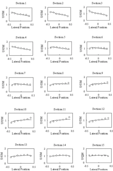
Fig. 2 shows the variation of velocity ratio U/UM across the dimensionless channel width Y/B obtained from simulated results and the measured data, where U = depth-averaged longitudinal ve-locity; UM is cross-section averaged longitudinal veve-locity; and Y/B represents the dimensionless lateral position 共B=channel width兲, where 0 is at the centerline, −0.5 is at the left bank, and 0.5 is at the right bank. One can observe from Fig. 2 that the simulated results have fairly good agreement with measured data. The velocity-distribution behavior is similar for the two bends in which one is from stations 2 to 8 and the other is from stations 10 to 15. In the entrance of the bend, the maximum velocities occur near the inner bank. As the flow moves farther downstream, the velocity distribution then begins to flatten out. The longitudinal velocity near the outer bank increases along the bend and the maximum velocity then shifts toward the opposite bank.

As pointed out by Almquist and Holley共1985兲, Elder 共1959兲, and Fischer et al. 共1979兲, formulas embedded in the present model were not suitable for the present case. Hence, by adjusting ␧␰and␧␩, which were assumed to be spatially variable along the channel, these two parameters can be calibrated by comparing measured and simulated concentrations in the case for injection near the left bank of station 2. By using the calibrated parameters, the accuracy of the suspension transport model was quantitatively assessed by comparing measured and simulated concentrations in the case for injection near the right bank of station 2. Fig. 3 shows the variation of concentration ratio C/Cmaxacross the lateral po-sition obtained from simulated results and the measured data in the case for injection near the right bank of station 2, where C = depth-averaged concentration; and Cmax= maximum depth-averaged concentration measured at that station and this value would decrease along the channel. From Fig. 3, one can find that model results consistently agree with measurements along the channel. The concentration peak keeps at the right bank in each

station. The lateral transport effect causes the tracer to move to-ward the left bank and the concentration distribution across the section approaches uniform gradually. In summary, from the above analyses, it is reasonable to positively conclude the model capability for the wash load transport process.

Fig. 1. Channel geometry and measured stations of suspension transport case关adapted from Almquist and Holley 共1985兲兴

Fig. 2. Lateral distribution of velocity ratio U/UM for Almquist and

Holley’s simulation

Degradation and Aggradation Cases for Noncohesive Sediment

The mechanism of degradation and aggradation for noncohesive sediment embedded in the present model are validated by com-paring the simulated results with experimental data obtained by Suryanarayana共1969兲.

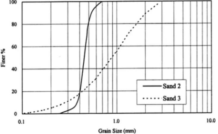
A straight flume having a rectangular cross section 18.3 m long and 0.6 m wide was used in Suryanarayana’s experiment. In the degradation case, the clean water with unit discharge 0.068 m2_{/s was specified at the channel inlet; the water-surface} elevation varied from 0.292 m to 0.302 m at the channel outlet. The particle gradation for the bed material and the sediment in-flow are shown in Fig. 4 and denoted as sand 3 and sand 2, respectively. In the aggradation case, the unit discharge and sedi-ment concentration of uniform sand 共sand 2 of Fig. 4, represen-tative diam is 0.45 mm兲 given at the upstream end of the channel were 0.024 m2/s and 409 ppm, respectively. The water-surface elevation at the downstream end of the channel was 0.257 m.

The uniform mesh of 51⫻5 was used in the simulation. The upstream boundary conditions were the inflow discharge per unit width and the sediment concentration. The measured water-surface elevation and the no-slip condition were used for the downstream end and the channel banks, respectively.

Fig. 5 shows the bed and water surface profile during degra-dation processes obtained from simulated results and measured data at t = 2.25 h, 7 h, and 13 h. By comparing the simulated and measured results in Fig. 5, it is evident that the simulated results have much less deviation from the measured data. From Fig. 5, one can also observe that water depth increases while bed slope decreases as degradation progressed. Bed degradation occurs mainly near upstream inlet at t = 2.25 h. As time increases, the process of bed degradation continuously progresses and passes on to the downstream; at t = 13 h, the degradation can be observed in the whole channel.

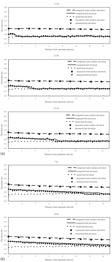
Fig. 6 shows the bed and water-surface profile during aggra-dation processes obtained from simulated results and measured data. In Fig. 6, the convincing agreement between the simulated results and measured data is observed. The excess sediment is deposited near the entrance of the stream because the sediment supply is grater than the transport capacity of the stream. The bed rises and the water depth and the slope of the bed increase, so that, to satisfy the updated hydraulic conditions, a new equilib-rium slope will be established. Meanwhile, a discontinuity of the bed can be observed with new equilibrium slope and can be called as aggrading front 共Suryanarayana 1969兲. Afterward, sediment enters the downstream of the aggrading front, the hydraulic con-ditions are not favorable enough for the sediment transported downstream, and, therefore, is deposited in this reach. Since there is a discontinuity near the aggrading front, the backwater effect is created and some part of the sediment would be deposited up-stream of the aggrading front. Thus, the deposition of sediment may proceed both upstream and downstream of the aggrading front. Finally, at t = 10 h, another new equilibrium slope is built over the whole stream and the stream can be considered as stable; no deposition or scouring occurs. Nevertheless, since the hybrid scheme adopted by the present study has only the first-order ac-curacy, the deviations between simulated results and measured data are larger near the shock front, as indicated in Fig. 6.

The studies demonstrated above show the capability of the present model to tackle the degradation and aggradation processes for noncohesive sediment. In order to further examine the trans-port mechanism of cohesive sediment embedded in the present

Fig. 3. Lateral distribution of depth-averaged concentration ratio

C/C_maxfor Almquist and Holley’s simulation

Fig. 4. Size gradation curve of Suryanarayana’s experiment

2.25 hr 0.10 0.15 0.20 0.25 0.30 0.35 0.40 0.45 0.50 0 2 4 6 8 10 12 14

Distance from upsteam end (m)

Elev

atio

n

(m)

computed waer-surface elevation computed bed elevation initial bed elevation measured bed elevation

7 hr 0.10 0.15 0.20 0.25 0.30 0.35 0.40 0.45 0.50 0 2 4 6 8 10 12 14

Distance from upstream end (m)

E leva ti on (m )

computed water-surface elevation computed bed elevation intial bed elevation measured bed elevation

13 hr 0.10 0.15 0.20 0.25 0.30 0.35 0.40 0.45 0.50 0 2 4 6 8 10 12 14

Distance from upstream end (m)

El

eva

tion

(m

)

computed water-surface elevation comuted bed elevation intial bed elevation measured bed elevation

Fig. 5. Variation of longitudinal bed profile with time共degradation case兲

model, a set of cohesive sediment cases is studied in the follow-ing paragraphs.

Degradation, Aggradation, and Consolidation Test for Cohesive Sediment

Due to lack of available experimental data for cohesive sediment in the literature, hereafter, a few specific hypothetical test cases are used to demonstrate the model’s capability.

Aggradation Process

The cases with straight rectangular channel by changing different inflow discharge, critical shear stress for deposition ␶cd, and in-flow concentration were studied. The channel has a length of 8,000 m, a width of 100 m, a slope of 0.0005, and Manning’s roughness of 0.03. The sediment data with three size classes: 0.001 mm共clay, 33.33%兲, 0.01 mm 共33.33%兲, and 0.05 mm 共silt, 33.33%兲 were chosen for this study. In each case, the water-surface elevation for the outlet of channel was fixed at 4.5 m, the zero initial concentration was used, the total simulation time was 6 days, and the mesh 81⫻11 was used in the simulation.

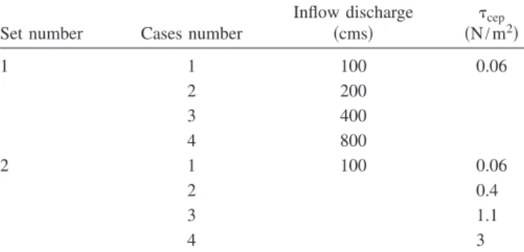
Three sets of scenarios with four various inflow discharge␶cd and inflow concentration, were designed and shown in Table 1.

The results of maximum aggrading height Hm and aggrading outset location Lo, which is equal to the distance from the up-stream end to the location of aggrading outset, obtained from the model are given in Table 2. For set 1, one can deduce that the bed shear stress␶bmay increase as inflow discharge increases and the chance for␶b⬍␶cdcorrespondingly decreases. Thus, one can ob-serve from Table 2 that Hmdecreases and Loincreases. This con-sequence indicates that the aggrading outset location moves downstream, from case 1 to case 4 of set 1. Similarly, the increase of␶cd may raise the probability of deposition; So, for set 2, Hm increases gradually and the aggrading outset location moves up-stream from case 1 to case 4 as shown in Table 2. The cases in set 3 only change the inflow concentration, in which the same flow condition and deposition criteria are considered. Hence, Lokeeps the same in each case and Hm increases due to the increase of inflow concentration from case 1 to case 4 of set 3, as shown in Table 2.

Degradation Process

The simulated conditions, including the geometry of channel, sediment data, water-surface elevation at the outlet of channel,

Table 1. Cohesive Sediment Data for Aggradation Simulation

Set number Case number Inflow discharge 共cms兲 共N/m␶cd2_兲 Inflow concentration 共ppm兲 1 1 2 0.06 2,000 2 8 3 16 4 24 2 1 24 0.06 2,000 2 0.10 3 0.40 4 1.10 3 1 24 0.06 2,000 2 4,000 3 6,000 4 10,000

Table 2. Results of Hm and Lo for Aggradation Cases of Cohesive Sediment

Case

Set 1 Set 2 Set 3

Hm共m兲 Lo共m兲 Hm共m兲 Lo共m兲 Hm共m兲 Lo共m兲 1 0.00087 0 0.00074 1,600 0.00074 1,600 2 0.00081 0 0.00078 1,000 0.00147 1,600 3 0.00077 800 0.00085 0 0.00220 1,600 4 0.00074 1,600 0.00088 0 0.00368 1,600 1.5 hr 0.10 0.15 0.20 0.25 0.30 0.35 0.40 0.45 0.50 0 2 4 6 8 10 12 14

Distance from upstream end (m)

E le va tio n (m )

computed water-surface elevation computed bed elevation intial bed elevation measured water-surface elevation measured bed elevation

2.5 hr 0.10 0.15 0.20 0.25 0.30 0.35 0.40 0.45 0.50 0 2 4 6 8 10 12 14

Distance from upstream end (m)

E leva ti on (m )

computed water-surface elevation computed bed elevation intial bed elevation measured water-surface elevation measured bed elevation

4.5 hr 0.10 0.15 0.20 0.25 0.30 0.35 0.40 0.45 0.50 0 2 4 6 8 10 12 14

Distance from upstream end (m)

E le vat ion (m )

computed water-surface elevation computed bed elevation initial bed elevation measured water-surface elevation measured bed elevation

7 hr 0.10 0.15 0.20 0.25 0.30 0.35 0.40 0.45 0.50 0 2 4 6 8 10 12 14

Distance from upstream end (m)

E le va tion (m )

computed water-surface elevation computed bed elevation initial bed elevation measured water-surface elevation measured bed elevation

10 hr 0.10 0.15 0.20 0.25 0.30 0.35 0.40 0.45 0.50 0 2 4 6 8 10 12 14

Distance from upstream end (m)

E le va tio n (m )

computed water-surface elevation computed bed elevation initial bed elevation measured water-surface elevation measured bed elevation

(b) (a)

Fig. 6. Variation of longitudinal bed profile with time共aggradation

case兲

initial concentration, and numerical parameters of the hypotheti-cal cases for the degradation process are the same as those men-tioned in the aggradation process. As shown in Table 3, the present study designs two sets of scenarios in the degradation process including four cases with various inflow discharge and ␶cep.

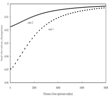
To test the influence of␶bon bed degradation, four cases of set 1 are designed by changing the inflow discharge. The bed profile simulated by the model shown in Fig. 7共a兲 indicates that the deg-radation depth increases gradually from case 1 to case 4. It is clear that the increase of inflow discharge would cause the in-crease of␶b, hence, the capability of bed degradation caused by the flow would increase correspondingly. The cases of set 2 are designed to test the influence of␶cepon bed degradation and the simulated results of bed profile are shown in Fig. 7共b兲. The prob-ability of bed shear stress exceeding ␶cep decreases when ␶cep

Table 3. Cohesive Sediment Data for Degradation Simulation

Set number Cases number

Inflow discharge 共cms兲 共N/m␶cep2_兲 1 1 100 0.06 2 200 3 400 4 800 2 1 100 0.06 2 0.4 3 1.1 4 3

(a) set 1

-0.06 -0.05 -0.04 -0.03 -0.02 -0.01 0 0.01 0 2000 4000 6000 8000

Distance from upstream end(m)

be d el ev at io n cha nge (m ) case1 case2 case3 case4

(b) set 2

Fig. 7. Bed elevation change for degradation test of cohesive sediment

increases, So as shown in Fig. 7共b兲, the change of bed level caused by degradation process becomes smaller from case 1 to case 4.

Consolidation Process

Two hypothetical cases are adopted to test the function of solidation processes embedded in the model. The simulated con-ditions of these two hypothetical cases are the same as the case 1 of set 1 mentioned in the degradation processes. The only differ-ence between two hypothetical cases is the treatment of ␶cepin each bed layer. The thickness of each bed layer is set as 1 cm. Case 1 ignores the consolidation effect and each layer specifies the same␶cepvalue as 0.06 N/m2; in contrast, case 2 takes into account the consolidation effect and each layer specifies different ␶cep, as shown in Table 4.

Fig. 8 shows the comparison of bed profile between simulated results for cases 1 and 2. One can observe from Fig. 8 that the maximum degradation depths for cases 1 and 2 are about 5 cm and 1.8 cm, which are located at the fifth and the second layer of initial bed, respectively. It is evident from simulated results that the degradation depth of case 2 is smaller than that of case 1 because the consolidation effect given in case 2 would suppress the bed degradation.

The phenomena interpretation analyzed above indicates a cer-tain extent of acceptability of the model for the simulation of cohesive sediment transport mechanism, although no experiment or field data are available for the validation.

Model Application

Study Goal

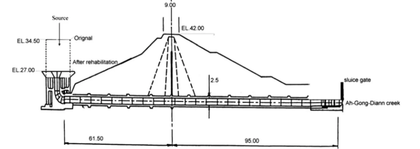
Ah Gong Diann Reservoir is located at southern part of Taiwan. Due to the loose characteristics of the soil within the catchment, a great amount of soil, in which more than 80% is of cohesive sediment, was carried into the reservoir with the surface runoff. According to the 1991 data, 71% of the storage is occupied by the sediment, which means about 500,000 m3_{of sediment was} depos-ited in the storage pond per year. Taiwan Water Resources Agency 共WRA兲 has proposed the “Ah Gong Diann Reservoir Rehabilita-tion Plan” to improve the capability and life of the reservoir. The rehabilitation plan suggested to lower the inlet of bell mouth spill-way down to near the bed level. Instead of flushing the flood, the reconstructed bell mouth inlet will be used to flush the inflow sediment. The layouts of the plan are shown in Figs. 9 and 10. The sluicing gate at the downstream of the tunnel will be opened during the flood season to sluice out the sediment from the reser-voir. Moreover, an off-basin diversion weir was constructed to sluice out the flood above the 100-year return period to the Niu-Chou-Pu Creek, located at another catchment near the Ah Gong Diann Reservoir.

Experimental Setup

An experiment 共WRA 1999兲 was conducted to model the sedi-ment flushing efficiency of the Ah Gong Diann Reservoir by fol-lowing the rehabilitation plan. The layout of the model is shown in Fig. 9. The Chuo-Shui Creek and Wang-Lai Creek inflow boundaries were located at transections 36 and 72, respectively. Based on the rehabilitation plan, the designed channel bed slopes are 4.63⫻10−3_{in river portion 共from transection 36 to 22兲 and} 1⫻10−3_{in reservoir portion共downstream the transection 22兲,} re-spectively. The sediment dredged from the Ah Gong Diann Res-ervoir is used for the experiment. In order to obey the dynamic similarity, the Froude number and the ratio of flow velocity and particle fall velocity at rest water, u/w, were used as the con-trolled dimensionless parameters. To avoid the scale effect, the distorted model, in which the horizontal and vertical scales were

Table 4. Cohesive Sediment Data for Consolidation Simulation

Layer number 1共top兲 2 3 4 5 6

Case 1␶cep共N/m2兲 0.06 0.06 0.06 0.06 0.06 0.06 Case 2␶cep共N/m2兲 0.06 0.2 1 2 3 3.5 -0.06 -0.05 -0.04 -0.03 -0.02 -0.01 0 0 2000 4000 6000 8000

Distance from upstream end(m)

b e d e lev a ti on c h ange ( m ) case 2 case 1

Fig. 8. Bed elevation change for consolidation cases of cohesive sediment

Fig. 9. Plan layout of Ah Gong Diann Reservoir

1:60 and 1:15, respectively, were used. The velocity ratio and Reynolds number between model and prototype were 1:3.87 and 1:60, respectively.

Treatment of Boundary Conditions

The general layout of the simulation area is shown in Fig. 11, in which the numbers represent the transection locations. There are three types of boundary in this study. Transections 36 and 72 are the Chuo-Shui Creek and Wang-Lai Creek inflow boundaries, re-spectively; the bell mouth spillway is an outflow boundary; and the other boundaries are solid wall conditions. The treatment of the inflow and solid wall boundaries have been mentioned previ-ously. Flow pattern near the bell mouth spillway in reality is 3D phenomena; obviously, the depth-averaged 2D model is inad-equate to explore the bell mouth outflow boundary effect to the flow domain. Nevertheless, for this study the major concern should be the long-term and wide-range evolution processes; the errors induced by the local and short-term effect can be ignored. Hence, the present study set a new outflow boundary, which is the interface section denoted aa⬘in Fig. 11, near the bell mouth spill-way to substitute the original outflow boundary. By adjusting the water-surface elevation, the outflow rate along the new outflow boundary can be controlled to have the same value as that of the

bell mouth spillway. The new outflow boundary is very close to the bell mouth spillway and the velocity nearby is very small due to the large depth. The influence on the flow and sediment trans-port phenomenon due to the virtual outflow boundary will be restricted in the local region near the outflow boundary, so the new substitute outflow boundary can be regarded as reasonable for the simulation. The new outflow boundary conditions for ex-periment and field are the water-surface elevation obtained from measured and reservoir routing, respectively.

Calibration for Numerical Model

The sediment-deposition amount measured along the channel in the experiment will be used to calibrate the parameters in the numerical model. The mesh of 92⫻14 is used in the simulation. The channel bed slope follows the requirement of rehabilitation plan. Three size classes: 0.172 mm 共fine sand, 2.73%兲, 0.02783 mm共silt, 67.58%兲, and 0.003873 mm 共clay, 29.69%兲 are chosen to represent the inflow sediment components. The values of␶cepand␶cemare set as 1.1089 N/m2共Teisson 1991兲 to reflect the long-term consolidation effect.

As mentioned previously, the sediment is mainly composed of silt and clay, So the mechanism of deposition for cohesive sedi-ment 共i.e., silt and clay) is the key for the model calibration.

Fig. 10. Cross-sectional layout of rehabilitation plan for bell mouth spillway

Fig. 11. Plan layout of simulation area

According to Eq.共10a兲, the deposition mechanism for cohesive sediment is subject to two factors, including critical shear stress for deposition␶cdand flocculation factor F, which appears in the cohesive sediment fall velocity formula. To investigate the effects of␶_cd and F on total sediment-deposition amount共kg兲 Msin the Ah Gong Diann Reservoir, a number of test cases are proposed herein for analyses. For each case, there is only one parameter varied while another variable remains fixed. The functional rela-tionship of Msand␶cdand F in a log-log scale is established as ln共Ms兲=C0+兺i=1Ciln共Di兲 with C0being a constant; Di represent-ing␶cdor F; and Cibeing the coefficient associated with Di. The coefficients obtained by the regression analysis are listed in Table 5. From Table 5, one can observe that F has a more significant effect on Msthan␶cd. Hence, the model is calibrated by adjusting F along the channel and␶cdwas set as a fixed value, 0.06 N/m2 共Krone 1962兲.

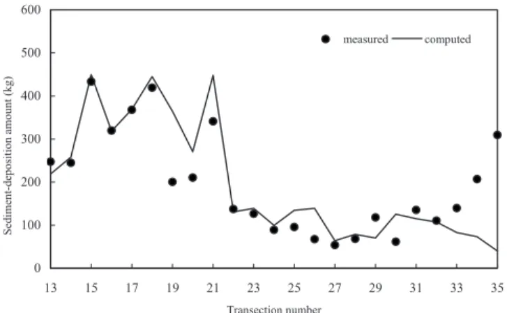
The 50-year return-period flood case is adopted to calibrate F along the channel. F is adjusted to achieve the best agreement between the simulated results and measured data. The calibrated result is given in Fig. 12, which shows the variation of sediment-deposition amount versus the transection number obtained from simulation and the measured data. One can observe from Fig. 12 that model results generally agree well with measured data except the region near the upstream end. In fact, the excessive deposition near the upstream end is the errors induced by experiments共WRA 1999兲 due to the difficulty of sediment inflow control. The values of F that yield the best model calibration results almost keep the same in the river portion; in contrast, these values increase from upstream to downstream in the reservoir portion.

The accuracy of the calibrated results is quantitatively as-sessed by using the data of the 5-year return-period flood case. Fig. 13 shows the corresponding sediment-deposition amount ver-sus the transection number obtained from simulation and the mea-sured data. As shown in Fig. 13, the convincing agreement between the simulated results and measured data is observed. The sediment-deposition amount is relatively small, below 100 kg, in the river portion; in contrast, the sediment-deposition amount be-comes larger in the reservoir portion due to the sudden increase of width, water depth, and decrease of velocity.

Efficiency of Sediment Control

After the parameters were validated, the model is applied to pre-dict the sediment-control efficiency of the proposed rehabilitation plan for the real case with various return periods flood. The mesh of 92⫻14 is used in the simulation.

Table 6 shows the simulated results of efficiency of the sedi-ment control Ei for various return periods, in which Ei can be defined as Ei= 1 − Ms/Mt, where Mt represents the total inflow sediment load 共kg兲. It has been found that Ei almost keeps the same, say about 42%, under 50-year return-period flood. Above 100-year return-period, Ei may increase as return period in-creases. As mentioned before, the off-basin diversion weir be-comes effective when the flood exceeds 100-year return period. The flood is diverted and the water-surface elevation near the downstream boundary during the flood may be reduced dramati-cally. Hence, the influence of the backwater effect may be lower and, as expected, the higher return-period flood should have higher efficiency of sediment control. In summary, the efficiency of sediment control after the rehabilitation plan is completed will reach approximately 56% for 1,000-year return period flood.

Conclusion

An unsteady 2D depth-averaged model for nonuniform sediment transport in alluvial channels has been presented in this paper. In this model, the orthogonal curvilinear coordinate system is

Table 5. Regression Coefficients of Total Sediment Load versus␶cdand F

Factor ␶cd F R2

Coefficient 4.53 16.47 99.8%

Table 6. Simulated Results of Sediment Control Efficiency for Ah Gong Diann Reservoir

Return period 共year兲 1,000 500 250 200 150 100 50 5 2 Ei共%兲 56.23 52.13 48 46.86 45.42 43.81 42.44 42.2 42.46 0 100 200 300 400 500 600 13 15 17 19 21 23 25 27 29 31 33 35 Transection number Se dim ent-de position am ount (kg) . measured computed

Fig. 12. Variation of sediment-deposition amount versus the transec-tion number for 50-year return period case

0 100 200 300 400 500 600 13 15 17 19 21 23 25 27 29 31 33 35 Transection number Se di m ent-d epos it ion am ount (k g ) . measured computed

Fig. 13. Variation of sediment-deposition amount versus the transec-tion number for 5-year return period case

adopted; the transport mechanisms of cohesive and noncohesive sediment are both embedded; the suspended load and bed load are treated separately. In addition, the computing processes for hy-draulic sorting, armoring, and bed consolidation are also included in the model. The model performance has been assessed through the comparison with experimental data and hypothetical test data. The assessment indicates that the model functions well.

The model’s applicability has been demonstrated through the application to the Ah Gong Diann Reservoir in Taiwan. Convinc-ing qualitative agreement is achieved between the predicted and observed trends in the sediment-deposition amount change for both the parameter calibration and validation processes. The effi-ciency of sediment control for the reservoir is numerically deter-mined by using the proposed model.

Acknowledgments

Partial financial support of this study from the National Science Council of Taiwan, R.O.C., through Contract No. NSC-89-2211-E009-031 and South Water Resources Office, Water Resources Agency, Ministry of Economic Affairs, Taiwan, R.O.C. are greatly appreciated. The experimental data provided by Water Re-sources Planning Institute, Water ReRe-sources Agency, Ministry of Economic Affairs, Taiwan R.O.C. is also appreciated. The com-puter resources used in this study were all executed on an IBM SP2 SMP machine, which was provided by the National Center for High-Performance Computing of Taiwan, R.O.C.

Notation

The following symbols are used in this paper: C ⫽ concentration;

Cd ⫽ near-bed deposition concentration; Ce ⫽ entrainment near-bed concentration; CF ⫽ coefficient;

Cf ⫽ friction factor; C0 ⫽ constant;

c ⫽ Chezy factor;

c₁ ⫽ grain Chezy coefficient; D ⫽ sediment diameter; Di ⫽ representing ␶cdor F;

Dm ⫽ smallest nonmoving size class; D₅₀ ⫽ median sediment-particle size; D

*k ⫽ dimensionless particle diameter;

d ⫽ water depth;

E ⫽ roughness parameter;

E_i ⫽ efficiency of the sediment control; Em ⫽ active-layer thickness;

e_␩ ⫽ lateral dispersion coefficient; F ⫽ flocculation factor;

F_d ⫽ characteristic depth of erosion; g ⫽ gravitational acceleration;

h1and h2 ⫽ metric coefficients in ␰ and ␩ directions, respectively;

M ⫽ material coefficient;

Ms ⫽ total sediment-deposition amount; p ⫽ porosity of the bed material;

Q1, Q2 ⫽ suspended-sediment flux due to both turbulent diffusion and lateral dispersion in the␰ and ␩ directions, respectively;

qb₁, qb₂ ⫽ components of bed-load flux in the ␰ and ␩ directions, respectively;

q_b

i

t

⫽ theoretical bed-load transport capacity in the i 共␰ or ␩兲 direction;

r ⫽ radius of curvature; S ⫽ suspended-sediment source; Sd ⫽ deposition component; Se ⫽ entrainment component; Sf ⫽ active-layer floor source;

s ⫽ dimensionless sediment density; Ti,j ⫽ integrated effective stress;

Tk ⫽ transport-stage parameter; t ⫽ time;

U_* ⫽ shear velocity;

u ⫽ ␰ components of velocity;

uw ⫽ depth-averaged velocity near the wall; u

* ⫽ effective bed-shear velocity;

u_*c ⫽ critical shear velocity evaluated from Shields diagram;

v ⫽ ␩ components of velocity;

ws ⫽ particle settling velocity following the Stokes law;

wl ⫽ lift-off velocity; wf ⫽ sediment fall velocity;

yw ⫽ distance between the first computational grid point adjacent to the wall and the wall itself; zb ⫽ bed elevation;

zs ⫽ water surface elevation; ␤ ⫽ active-layer size fraction; ␤s ⫽ active stratum size fraction; ⌬t ⫽ time step;

␧␰and␧␩ ⫽ turbulent diffusion coefficients in the ␰ and ␩ directions, respectively;

␨ ⫽ hiding factor;

␰ and ␩ ⫽ orthogonal curvilinear coordinates in streamwise axis and transverse axis, respectively;

␳ ⫽ fluid density; ␳d ⫽ bulk density; ␳s ⫽ density of sediment;

␶b1,␶b2 ⫽ ith direction components of free-surface and bed-shear stress, respectively;

␶cd ⫽ critical shear stress for deposition;

␶cem ⫽ critical bed shear stress for mass erosion; and ␶cep ⫽ critical shear stress for particle erosion. Superscripts

n ⫽ variables at time level n;

n + 1 ⫽ variables at time level 共n+1兲⌬t; and 共ញ兲 ⫽ depth average.

Subscripts

b ⫽ dependent variables at channel bed; k ⫽ kth size class; and

s ⫽ dependent variables at the water surface.

References

Almquist, C. W., and Holley, E. R.共1985兲. “Transverse mixing in mean-dering laboratory channels rectangular and naturally varying cross-section.” Technical Rep. No. 205, Center for Research in Water Resources, Univ. of Texas at Austin, Austin, Tex.

Ariathurai, R.共1974兲. “A finite element model for sediment transport in estuaries.” Ph.D. thesis, Dept. of Civil Engineering, Univ. of Califor-nia, Davis, Calif.

Bennett, J. P., and Nordin, C. F.共1977兲. “Simulation of sediment transport and armoring.” Hydrol. Sci. Bull., 37, 2119–2162.

Biglari, B., and Sturm, T. W. 共1998兲. “Numerical modeling of flow around bridge abutments in compound channel.” J. Hydraul. Eng.,

124共2兲, 156–164.

Borah, D. K., Alonso, C. V., and Prasad, S. H.共1982兲. “Routing graded sediments in streams: Formulations.” J. Hydr. Div., 108共12兲, 1486– 1505.

Celik, I., and Rodi, W.共1988兲. “Modeling suspended sediment transport in nonequilibrium situations.” J. Hydraul. Eng., 114共10兲, 1157–1191. Elder, J. W.共1959兲. “The dispersion of marked fluid in turbulent shear

flow.” J. Fluid Mech., 5共4兲, 544–560.

Fang, H. W., and Wang, G. Q.共2000兲. “Three-dimensional mathematical model of suspended-sediment transport.” J. Hydraul. Eng., 126共8兲, 578–592.

Fischer, H. B., List, E. J., Koh, R. C. Y., Imberger, J., and Brookes, N. H. 共1979兲. Mixing in inland and coastal waters, Academic, San Diego. Holly, F. M., and Rahuel, J. L.共1990兲. “New numerical physical

frame-work for mobile-bed modeling.” J. Hydraul. Res., 28共4兲, 401–416. Hsieh, T. Y., and Yang, J. C.共2003兲. “Investigation on the suitability of

2D depth—Averaged models for bend-flow simulation.” J. Hydraul.

Eng., 129共8兲, 597–612.

Hsieh, T. Y., and Yang, J. C. 共2004兲. “Implicit two-step split-operator approach for modelling two-dimensional open channel flow.” J.

Hy-drosci. Hydr. Eng., 22共2兲, 113–139.

Hsieh, T. Y., and Yang, J. C. 共2005兲. “Numerical examination on the secondary-current effect for contaminant transport in curved channel.”

J. Hydraul. Res., 43共6兲, 643–658.

Hu, C., and Hui, Y.共1996兲. “Bed-load transport. I: Mechanical character-istics.” J. Hydraul. Eng., 122共5兲, 245–254.

Karim, M. F., Holly, F. M., and Yang, J. C.共1987兲. “IALLUVIAL: Nu-merical simulation of mobile-bed rivers. Part I. Theoretical and nu-merical principles.” Rep. No. 309, Iowa Institute of Hydraulic Research, Univ. of Iowa, Iowa City, Iowa.

Kassem, A. A., and Chaudhry, M. H. 共2002兲. “Numerical modeling of bed evolution in channel bends.” J. Hydraul. Eng., 128共5兲, 507–514. Krone, R. B.共1962兲 “Flume studies of the transport of sediment in estua-rine shoaling processes.” Technical Rep., Hydraulic Engineering Lab., Univ. of California, Berkeley.

Lane, E. W., et al. 共1974兲. “Report of the subcommittee on sediment terminology.” EOS Trans. Am. Geophys. Union, 128共6兲, 936–938. Li, C. W., and Ma, F. X.共2001兲. “3D numerical simulation of deposition

patterns due to sand disposal in flowing water.” J. Hydraul. Eng.,

127共3兲, 209–218.

Lin, B. 共1984兲. “Current study of unsteady transport of sediment in China.” Proc., Japan-China Bi-Lateral Seminar on River Hydraulics

and Engineering Experiences, 337–342.

Migniot, C. 共1989兲. “Bedding-down and rheology of muds. Part I.”

Houille Blanche, 1, 11–29共in French兲.

Partheniades, E.共1965兲. “Erosion and deposition of cohesive soils.” J.

Hydr. Div., 91共1兲, 105–139.

Rastogi, A. K., and Rodi, W.共1978兲. “Prediction of heat and mass trans-fer in open channels.” J. Hydr. Div., 104共3兲, 397–420.

Rijn, L. C., Rossum, H., and Termes, P.共1990兲. “Field verification of 2-D and 3-D suspended-sediment models.” J. Hydraul. Eng., 116共10兲, 1270–1288.

Shimizu, Y., and Itakura, T.共1989兲. “Calculation of bed variation in al-luvial channels.” J. Hydraul. Eng., 115共3兲, 367–384.

Spasojevic, M., and Holly, F. M.共1990兲. “2-D bed evolution in natural watercourses—New simulation approach.” J. Waterway, Port, Coastal, Ocean Eng., 116共4兲, 425–443.

Struiksma, N. 共1985兲. “Prediction of 2D bed topography in rivers.” J.

Hydraul. Eng., 111共8兲, 1169–1182.

Suryanarayana, B.共1969兲. “Mechanics of degradation and aggradation in a laboratory flume.” Engrg. hydr., Colorado State Univ., Fort Collins, Colo.

Teisson, C.共1991兲. “Cohesive suspended sediment transport: Feasibility and limitations of numerical modeling.” J. Hydraul. Res., 29共6兲, 755– 769.

Thomas, W. A., and McAnally, W. H. 共1985兲. User’s manual for the

generalized computer program system open-channel flow and sedi-mentation TABS-2, Dept. of the Army Waterways Experiment Station,

Corps of Engineers, Vicksburg, Miss.

Van Rijn, L. C.共1984a兲. “Sediment transports. Part I: Bed load transport.”

J. Hydraul. Eng., 110共10兲, 1431–1456.

Van Rijn, L. C. 共1984b兲. “Sediment transports. Part II: Suspended load transport.” J. Hydraul. Eng., 110共11兲, 1613–1641.

WRA. 共1999兲. “Hydraulic model study of the desilting functions of sluiceway in Ah Gong Diann Reservoir.” Technical Rep., Water Re-sources Planning Institute, Water ReRe-sources Agency, Ministry of Eco-nomic Affairs, Taiwan, R.O.C.共in Chinese兲.

Wu, W., Rodi, W., and Wenka, T. 共2000兲. “3D numerical modeling of flow and sediment transport in open channels.” J. Hydraul. Eng.,

126共1兲, 4–15.

Ziegler, C. K., and Nisbet, B. S.共1995兲. “Long-term simulation of fine-grained sediment transport in large reservoir.” J. Hydraul. Eng.,

121共11兲, 773–781.