國
立
交
通
大
學
多媒體工程研究所
碩
士
論
文
以樣本學習的紋理合成技術
擴增三維物件於繪畫中之演算法
Augmented 3D Object in Painting by
Example-based Texture Synthesis
研 究 生:邱雅菁
指導教授:莊榮宏 教授
林正中 教授
以樣本學習的紋理合成技術擴增三維物件於繪畫中之演算法
Augmented 3D Object in Painting by
Example-based Texture Synthesis
研 究 生:邱雅菁 Student:Ya-Ching Chiu 指導教授:莊榮宏 Advisor:Jung-Hong Chuang 林正中 Cheng-Chung Lin 國 立 交 通 大 學 多 媒 體 工 程 研 究 所 碩 士 論 文 A Thesis Submitted to
Institute of MultimediaEngineering College of Computer Science National Chiao Tung University in partial Fulfillment of the Requirements
for the Degree of Master in
Computer Science
July 2007
Hsinchu, Taiwan, Republic of China
以樣本學習的紋理合成技術
擴增三維物件於繪畫中之演算法
研究生:邱雅菁
指導教授:莊榮宏 博士
林正中 博士
國立交通大學資訊學院
多媒體工程研究所
摘要
我們提出了一個用區塊紋理合成技術為基礎的架構,將一幅繪畫作品風格 轉換到 3D 物件上,並且使 3D 物件能夠與繪畫作品融合,讓物件彷彿是繪 畫作品中原本的物件。利用紋理合成的和色彩轉換的技術,將繪畫作品的 風格轉換到 3D 物件的投射影像。透過基本顏色類別的分類,和統計學的 分析方法,將 3D 物件的投射影像的色彩轉換,使之能與繪畫作品的色調 相仿。然後,我們提出了新的二回合紋理合成架構(Two-passes Texture Synthesis ), 與可以改變筆觸走向的方向場貼圖(direction field),將繪畫作 品的筆觸轉移到 3D 物件的投射影像上。如此在 3D 物件的投射影像上所合 成的筆觸可以隨著 3D 物件表面起伏而改變,能夠更自然的模擬畫家描繪 真實物體時的筆觸。我們的系統可以將繪畫作品的風格成功的轉移到另外 物件上,讓物件能夠與繪畫作品相融。Augmented 3D Objected in Painting by
Example-based Texture Synthesis
Student: Ya-Ching Chiu
Advisor: Dr. Jung-Hong Chuang
Dr. Cheng-Chung Lin
Institute of Multimedia and Engineering
College of Computer Science
National Chiao Tung University
Hsinchu, Taiwan, R.O.C.
Abstract
We present a patch-based texture synthesis framework to accomplish our goal to immerse a 3D object into a 2D example painting. By texture synthesis and color transfer technique, the style of the example painting is transferred to the 3D projected image. The color transfer is automatically accomplished by basic color categories and statistical analysis of example painting and projected image. After color transfer, the projected painting can have similar color tone of the example painting. We proposed a new two-pass texture synthesis framework can transfer the stroke of the example painting to the projected painting. The new framework
improves the expression of the stroke according to the luminance of the projected painting. We also propose a novel approach to compute a continuous direction field, which can change the direction of the stroke that synthesized on the projected image. Thus the stroke will seem more natural and vivid in projected image, like the real stroke drawn by a painter. Our system could transfer the style of the example painting well and immerse the 3D object into a painting seamlessly.
ACKNOWLEDGMENT
I would like to thank my advisor, Professor Jung-Hong Chuang and Professor. Tsai-Pei Wang, who are always available and attentive, and patiently guided me through the steps of my master’s degree. Their comments and encouragements help me accomplish this thesis. I am grateful to my colleagues in lab: Tan-Chi Ho, Horng-Shyang Liao, Ji-Wen Chon, Yu-Shuo Lio, Chia-Lin Ko, Yung-Cheng Chen, Yueh-Tse Chen, Chih-Hsiang Chang, Hsin-Hsiao Lin, Kuang-Wei Fu, and
Ying-Tsung Li, helping me a lot in research and lab business. Thanks for my cute friends, Bing-Jhen Wu, Ya-Lin Huang, Hui-Chen Lin. Their accompany comfort me during those depressed and hard time. It is good to have Shin-Yao Chen, Zih-Ying Liou, Shin-Yin He and Guang-Hong Yang to stand by me.
Last, and the most important, I would like to thank my family. Their care and love support me and strengthen me, make me come through this.
Content
List of Figures vi 1 Introduction...1 1.1 Motivation...1 1.2 Overview...1 1.2.1 Style Transferring...2 1.2.2 Color Transfer ...2 1.3 Organization...3 2 Related Work...4 2.1 Augmented Reality of NPR ...4 2.2 Example-based Rendering ...6 3 Methods...9 3.1 System Overview ...9 3.2 Color Transfer ...103.2.1 The color transfer process ... 11
3.2.2 Generate Indirect Color Category ...14
3.3 Texture Synthesis ...16
3.3.1 One-Pass Texture Synthesis ...17
3.3.2 Two-Pass Texture Synthesis Framework ...21
3.3.3 Direction Field ...23
3.4 Composite Projected Image into Example Painting ...27
4 Results ...28
4.1 Result of color transfer and direction field ...28
5 Conclusion ...35
5.1 Summary ...35
5.2 Future Work ...36
List of Figures
Figure 2.1 The 3D mesh are constructed and be rendered by different style... 5
Figure 2.2 The same light condition but different style of Venus model. ... 5
Figure 2.3 The result of Fischer et al. work. ... 6
Figure 2.4 The different style of AR application. ... 6
Figure 2.5 The result of Image Analogies. ... 7
Figure 2.6 The comparison of results different texture synthesis. ... 7
Figure 2.7 The example of texture transfer proposed by Efros and Freeman. ... 8
Figure 2.8 The result of work of Bin Wang et al... 8
Figure 3.1 The system overview ... 10
Figure 3.2 The flow char of color transfer procedure. ... 12
Figure 3.3 Color circle. [CSU+04]... 15
Figure 3.4 The illustration of one-pass texture synthesis... 18
Figure 3.5 The cell division example. ... 19
Figure 3.7 Synthesis order... 20
Figure 3.8 The three conditions of boundary area. ... 21
Figure 3.9 Comparison of the two passes. ... 22
Figure 3.10 The comparison of one-pass and two-pass framework... 23
Figure 3.11 The difference of direction field of Wang et al. and our work... 24
Figure 3.12 The procedure of direction field.. ... 25
Figure 3.13 The method to project tangential vector to direction field... 26
Figure 3.14 The direction field result... 26
Figure 3.15 The composition example... 27
Figure 4.1 The comparison of the color transfer.. ... 29
Figure 4.2 We put one cat model into the painting in the right bottom corner... 30
Figure 4.3 Comparison of the results with and without the direction field... 31
Figure 4.4 The effect of two-pass texture synthesis... 31 Figure 4.5 (a) The example painting. The dotted-line square is the sample textures. (b)
The object we put into the painting (the color has been transformed). (c) The final result. ... 32 Figure 4.6 (a) The example painting (b) The Cessna airplane model(top) and the image have the same style of the example painting(bottom) (c) The final result ... 33 Figure 4.7 (a) A water color painting. (b) The result of augmented painting with a Cessna plane ... 34
1
C H A P T E R 1
Introduction
1.1 Motivation
The non-photorealistic rendering (NPR) is a unique and interesting topic in
computer graphics. Unlike the simulation of physical phenomena and photorealistic rendering, NPR can generate amazing result without complicated mathematical equations. Many applications of NPR try to simulate the artistic style in various forms of artwork, for example, the water color, oil painting, pan-and-ink effects, or the impressionism style. Most previous works focus on 2D images or 3D model applications, with less concern in the interactive interaction between image and user. Recently, inspired by animating picture with stochastic motion texture [CGZ+05], the interaction with 2D images, such as moving of objects in a 2D painting, is a novel and useful application.
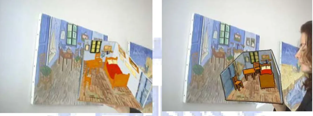
We present a framework to accomplish the goal of interacting with objects in a 2D painting. The goal is to insert objects into a given painting, with the inserted objects rendered in the same style of the painting, and to move or rotate the objects in the painting.
1.2 Overview
Our research goal is to propose a framework that allows user to add a 3D object into a painting, immerse the object with the painting seamlessly by applying the texture transformation techniques [EL03], and to interact with those objects. In the previous work of Fischer et al. [FBS05], to improve the immersion of a 3D model into the painting, both the 3D model and the example painting are rendered with the same
style. However, in our framework, the object is inserted a given painting and rendered with the same style of the painting. Texture synthesis and color
transformation technique are used to transfer the style of the example painting to the 3D object. We also introduce a 2D map called direction field during the texture transfer process to guide the stroke direction. In addition to the texture transfer, the color of the 3D object is adjusted as well to match the color scheme of the example painting.
1.2.1 Style Transferring
Style transferring has been studied by many computer graphics and image processing works. The problem of style transferring is that the style of the output should be perceived by human observers to be the same style of the source.
We use the patch-base texture synthesis approach to transfer the style of the example painting to the object. The painting style of brush stroke of in the example painting is represented by some blocks of the sample textures which are selected by users manually. By applying patch-based texture synthesis approach with the sample textures, the brush stroke of the example painting is synthesize to the target image of inserted object, i.e. the projected image. However, the strokes are directional. When a painter draws an object, stroke direction has to change in order to better express the objects. To this end, Bin Wang et al. have proposed a direction field that is derived by using the medial axis of segmented areas in the painting. Since only object contour is taken into account, the derived direction field cannot reflect the shape of the object. Alternatively, we take the 3D model surface curvature into account and derive a direction field that is able to better reflect the shape of object. With the proposed direction field, the synthesized strokes for the inserted objects are more convincing, and better express the style of the original example painting.
1.2.2 Color Transfer
Color is one of the most influential and powerful elements in images and a variety of color processing methods have been proposed in the field of image processing. It is also a significant feature for people to identify the style of artworks. To increase the immersion of the inserted 3D objects with the example painting, the color of the 3D objects has to be adjusted so that the color tone of the projected image will agree with that of the example painting. To capture the characteristics of color used in the example painting, we use the color classification method proposed by Y.Chang et al.
[CSU+04]. By defining 11 basic color categories and classify each pixel color into 11 categories, we can capture the characteristics of each color unit of the example painting. This method takes the color mixing with surrounding colors effect into account [Fai1997], so that the characteristics of color unit we found will conform to the human color perception in real environment.
1.3 Organization
This thesis is organized as follows. Chapter 2 provides a brief introduction of the related works: augmented reality and example-based rendering. Chapter 3 presents our proposed framework and the implementation detail for each component in the framework. Chapter 4 presents the result of our work, and finally, Chapter 5 concludes and describes possible direction of future work
2
C H A P T E R 2
Related Work
In this chapter, we introduce some related works about augmented reality (AR) and example-based rendering applications. Since we try to put a virtual 3D object into a real painting, the goal is similar to the augmented reality. The difference between our work and traditional AR applications is that the environment where the 3D object is placed is not a photo of real scene but a painting. We show some previous works with different NPR techniques to combine the real world and the virtual object. Another related topic is the example-based rendering, where the output has some similarity of the input example. Then we introduce some techniques about texture synthesis.2.1 Augmented Reality of NPR
Augmented reality (AR) is a growing field in computer graphics and virtual reality. Most augmented reality applications are concerned with the use of photos or video with additional objects which are computer generated. However, AR applications usually focus on photorealistic rendering by using soft shadow, reflection, and lighting techniques to improve the sense of reality in scene. Our system is the same as AR that we want to augment object in a static environment, a painting. The difference between traditional AR and our application is that the virtual object has to be rendered with artist style.
Compared with augmented reality application with photorealistic rendering, there are much less AR applications of NPR than traditional AR applications. Haller and Sperl propose a system to create an impressionistic image by stroke brush [HS04]. Their painting system creates a painterly image by using brush strokes which obtain their attributes (position, color, size) from a reference picture, such as photos or paintings, and then they render a 3D object or scene by painterly system.
Figure 2.1 is the example of Haller and Sperl’s work. The 3D mesh model of the Van Gogh’s painting is constructed, and the brush attribute is computed by the painting. The 3D model is rendered by the painterly brush, and user can change the model’s render style. Their system does not try to immerse the virtual object into a real world or paint, but apply different painting style to the 3D model. In this work, they can also abstract the light model from a photo and render the virtual object with the same lighting condition. Figure 2.2 is the example of Venus with different style, and rendered with the light from the background photo.
Figure 2.1 The 3D mesh are constructed and be rendered by different style. In left image, the model is rendered by oil painting style, and in right image, the model is rendered by cartoon-like style.
Figure 2.2 The same light condition but different style of Venus model.
In 2005, Fischer et al. propose a novel approach for generating augmented reality images [FBS05]. They apply a painterly image filter to the video stream, and the virtual object is rendered with the same style of the filter by NPR technique, as Figure 2.3 shows. Thus the user can feel the virtual object is part of the real
surrounding. Figure 2.4 display the ability of their system to render with different NPR style.
(a) (b) Figure 2.3 The result of Fischer et al. work. (a) The tea pot is virtual object and the
background image is real scene. (b) Both tea pot and background image is rendered by cartoon-like style. [FBS05]
(a) (b) Figure 2.4 The different style of AR application. (a) The real video stream and virtual cut scene. (b)
The sketch-like stylization. [FBS05]
2.2 Example-based Rendering
Example-based rendering is an approach that is applied in many applications in computer graphics. The feature of this approach is that the rendering output has a specific feature which is related to the input example. The example is usually a 2D image or 3D model, and sometimes the video stream will be used as example as well. Many NPR applications apply example-based approach to synthesis artistic effect, and furthermore these applications usually use texture synthesis techniques. Image Analogies proposed by Hertzmann et al. is one famous work, and it generates a very broad range of artistic effects [HJO+01]. They use one pairs of images, where one is the original image and the other is a filtered version of original
image, as input example, and then apply the same filter effect to another image. Figure 2.5 is the result of image analogies with water color effect. In this work, Hertzmann et al. take two kind of pixel-based texture synthesis schemes:
approximate search and coherence search, and use a coherence parameterκto decide which search result of the two search schemes will be adapt. The output pair image B’ is synthesized from B with the same texture synthesis parameter.
A A’ B B’
Figure 2.5 The result of Image Analogies. The A, A’ and B image are three input images, and the result image B’ has the same variation from B just as the variation from A to A’. [HJO+01]
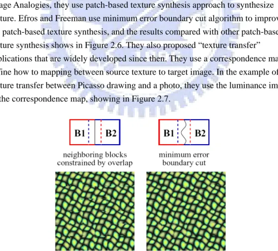
In 2001, Efros and Freeman present a simple image-based method to transfer texture from one source texture to another target image [EF01]. Different from the Image Analogies, they use patch-based texture synthesis approach to synthesize texture. Efros and Freeman use minimum error boundary cut algorithm to improve the patch-based texture synthesis, and the results compared with other patch-based texture synthesis shows in Figure 2.6. They also proposed “texture transfer”
applications that are widely developed since then. They use a correspondence map to define how to mapping between source texture to target image. In the example of texture transfer between Picasso drawing and a photo, they use the luminance image as the correspondence map, showing in Figure 2.7.
overlapping and (b) the result of minimum error boundary cut. [EF01]
(a) (b) (c) Figure 2.7 The example of texture transfer proposed by Efros and Freeman. They
use patch-based texture synthesis technique to transfer the texture from the source texture to target image. [EF01] (a) source texture, the Picasso drawing, (b) target image, a photo of Feymman, (c) The result of texture transfer
Following the idea of luminance mapping, Bin Wang et al. 2004 propose a system to transfer style from one example painting to a photo image. They use patch-based texture synthesis with Gaussian pyramid acceleration, and selecting sample textures from the example painting. They also improve the method used in [GCS02] to generate a direction field of the photo image. The direction field
describes the contours of object in the photo, and decides the direction of the strokes. So the strokes are synthesized along the contours of objects in photo image,
resulting in visual appearance of the synthesized painting. Figure 2.8 is the result of Bin Wang et al.
(a) (b) (c)
Figure 2.8 The result of work of Bin Wang et al.. (a) photo image (b) example painting (c) result synthesized image [WWY+04]
3
C H A P T E R 3
Methods
In this Chapter we explain how to transfer the color scheme and stroke from the example painting to the projected image. The color scheme is the tendency of the color. First, we analyze the color scheme of the example painting, and change the color of the projected image into similar color tendency of the example painting. Second, the strokes of the example painting are transfer to the projected image by patch-based texture synthesis techniques. We start from the color transfer technique that changes the color of the projected image; then introduce our method tosynthesize stroke on the projected image with the direction field.
3.1 System Overview
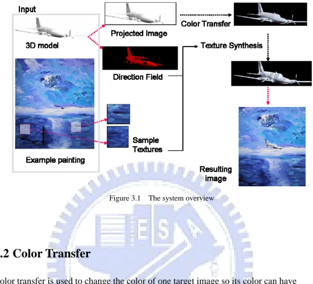
Figure 3.1 displays the overview of our system. The inputs of the system are one 2D example painting and one 3D model. The user first selects some rectangular areas from the example painting as sample textures, which are used as the source of texture while texture synthesis processing. The 3D object is projected to a 2D image, called the projected image, and the tangential vectors on the model surface are project to the direction field as well. The projected image has to change its color by color transfer, so that it has the same color scheme as the example painting. We then synthesized the stroke to the projected images so the stroke style of the example painting would transfer to the projected image. Finally, putting the projected image to the example painting, the 3D model would seems an original objected in the painting
The section 3.2 will introduce the color transfer technique we used in our framework, following detail of the texture synthesis technique in section 3.3. The method of generating direction field will also described in section 3.3.3.
Figure 3.1 The system overview
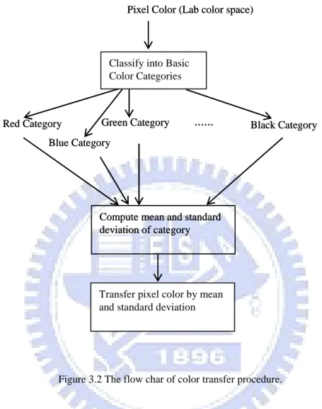
3.2 Color Transfer
Color transfer is used to change the color of one target image so its color can have the same characteristic of a reference image. In our system, the target image is the projected image and the reference image is the example painting. To imitate the style of the example painting, our system has to transfer the color characteristic of the painting to the projected image as well because color is a one of the major feature to recognize a style. If the 3D object has different color scheme from the paintings, viewer will not feel that the object has the same style of the painting. For example, a bright blue object appears in a painting with pale yellow tone, the object cannot immerse into the painting well. For this reason, the added 3D object has to change its color to immerse into the painting.
There are two tasks in color transfer: color correspondence between images and color transfer in target image. Color correspondence is finding an example color from the reference image for each pixel in target image, and the target image can change its pixel color into a similar tone of corresponding color. For example, the yellowish grass area in target image may map to the deep green forest area in the reference image because these two areas have similar hue. Then the grass will become darker green, like the forest in the reference image.
luminance mapping [RAG+01][WAM02][LLW04]. They segment image by clustering pixels with similar color and assign the corresponding color to each cluster. The luminance mapping is to fine the pixels with closest L2 distance of luminance value, and set them as corresponding pixel color to the target image. However, there are two problems of such process: 1. if the target image has some pixel colors which do not exist in reference image, the result of transfer may be inharmonious; 2. those methods need user effort to find a better mapping if the result of color transfer is wrong or unnatural, and the user needs have good aesthetic sense to map proper colors.
In our system, we use the basic color category proposed by Change et al. [CSU+04] to find the appropriate mapping between images automatically. Basic color categories can be used to classify pixel color and find the corresponding color according to human visual perception. Then the result of color transfer seems much natural.
After finding the corresponding color in the reference image, the next step of color transfer is adjusting the color value of the target image so its tone can near the reference image. We adapt the statistical analysis of the Reinhard et al. and scale the pixel color of target image according to the mean and ratio of standard deviation of each color category [RAG+01].
3.2.1 The color transfer process
Figure 3.2 is the process of color transfer in our system. First, the representation of pixel color are converted from the RGB to the CIEL*a*b* color space. The channels of RGB color space are correlated, so the changing of color will affect three
channels.On the other hand, CIEL*a*b* color space is an orthogonal color space without correlation between axes. If we only want to change the luminance of the pixel, we can consider the L channel without considering the other two channels. Besides, uniform changing of channel will be detected equally in orthogonal color space.
After both the projected image and example painting are converted from RGB color space to CIEL*a*b* color space, the pixels are classified into 11 basic color categories. The concept of basic color categories are originally reported by Berlin and Kay [BK69]. They study nearly 98 languages and find 11 most common color terms called Basic Color Terms (BCTs). For example, the 11 terms in English are white, black, red, blue, green, yellow, purple, pink, orange, brown and gray. In 2004, Chang et al. define 11 basic color categories according to the 11 BCTs. They divide
the color space into 11 categories, and define the range of each color category in color space.
Classify into Basic Color Categories
Pixel Color (Lab color space)
Red Category
Blue Category
Green Category ... Black Category
Compute mean and standard deviation of category
Transfer pixel color by mean and standard deviation
Classify into Basic Color Categories
Pixel Color (Lab color space)
Red Category
Blue Category
Green Category ... Black Category
Compute mean and standard deviation of category
Transfer pixel color by mean and standard deviation
Figure 3.2 The flow char of color transfer procedure.
We adopt their definition of color range for 11 color categories in our system. When Change et al. test the color range of basic categories, they consider one important phenomenon: the appearance of color is often affected by surrounding color. Especially for the color with low saturation, the color shift will be more apparent. The range or achromatic color category, i.e. the white, black and gray categories, are expanded in Change et al. experiment. Thus the color range of basic categories much conforms to the human perception.
In our system, the CIEL*a*b* are divided into 11 regions which is mutual exclusive. Both the pixel colors of projected image and example painting are
classified into color category, and each pixel color treat as a site in CIEL*a*b* color space; if one site are inside the one region of category Ci means the pixel color are
automatically find the proper mapping in the example painting. For example, the pixel color in blue category will map to the color in blue category of the example painting.
Next, we change the color distribution of each category of the projected image to imitate the color use of the example painting. This is the same as the statistical analysis process proposed by Reinhard et al. [RAG+01]. For one color categoryCi,
we compute its mean and standard deviation, as the equation 3.1and 3.2 shows:
i i C C N k k L N L
∑
= = 1 μ , i i C C N k k a N a∑
= = 1 μ , i i C C N k k b N b∑
= = 1 μ (3.1) , ) ( 1 2 i i C C N k L k L N L∑
= − = μ ρ , ) ( 1 2 i i C C N k a k a N a∑
= − = μ ρ , ) ( 1 2 i i C C N k b k b N b∑
= − = μ ρ (3.2)The superscriptCiis the one basic color category, where i={red, blue, green, yellow,
pink, purple, orange, brown, white, black, gray};N is the total pixel color number Ci of color categoryCi; the subscript L, a, and b means the three channel of CIEL*a*b*
color space, respectively; μandρare the mean and the standard deviation of a color category; Lk, akand bkare the L, a, and b channel of one color site k in color
categoryCi. Then the every new color site in Ciof projected image is computed by
the following equation:
ref L ref L in L in L in result L L μ σ σ μ × + − =[( ) ] ref a ref a in a in a in result a a μ σ σ μ × + − =[( ) ] (3.3) ref b ref b in b in b in result b b μ σ σ μ × + − =[( ) ]
where the superscript in , ref and resultmeans projected image, the example painting and the result respectively. After this transformation, the resulting pixel colors have standard deviations that conform to the example painting. We then add
the mean of example painting to shift the color more like the example painting.
3.2.2 Generate Indirect Color Category
Sometimes, the projected image has some pixel color belongs to a basic color category Ci which no pixel color of the example painting belongs to. In this case,
the distribution for color category Ci has to be automatically estimated by other
basic categories of example painting. We use the same method proposed in Chang et al. work. Only the mean μCiand the standard deviation σCiof Ciare needed
because we use these two statistical properties to compute color transfer. The mean
i
C
μ
is a color site too, so we use HSV color space to compute it because the HSV
color space separates the hue channel. Thus we could estimate μCi easily because
the saturation and brightness are easily computed by interpolation, and the hue can be decided by a simple equation. The values of saturation and brightness for mean
i
C
μ
are estimated by equation 3.4 and 3.5:
), ( ) ( ( ) ( ) ( Cuniv T j ref C j univ C ref Ci S i w S j S j S μ = μ +
∑
μ − μ ∈ (3.4) ) ( ) ( ( ) ( ) ( Cuniv T j ref C j univ C ref Ci B i w B j B j B μ = μ +∑
μ − μ ∈ (3.5)where the ci is the center of color category, and the T is the set of basic color
categories which exist in the example painting. The superscript ref, univ mean the reference image and universal color respectively.
Figure 3.3 Color circle. [CSU+04]
Because H not a linear mapping value, we cannot estimate H value by linear interpolation. We calculate the values of yellowish(y), bluish (b), and reddish(r) separately for each category in T . The Figure 3.3 present how the three terms can describe the color shift in the color circle. For example, if red become yellowish, then it becomes orange; if the blue become reddish, then it becomes purple. The variation of the three variables can calculate by equation 3.6:
T j c H c H w x= j( ( refj )− ( univj )), ∈ : : : : : : : : pink j brown j purple j blue j green j yellow j orange j red j = = = = = = = = ) 0 ( ) 0 ( ) 0 ( ) 0 ( ) 0 ( ) 0 ( ) 0 ( ) 0 ( ≥ ≥ ≥ ≥ ≥ ≥ ≥ ≥ x if x if x if x if x if x if x if x if x r r x y y x r r x r r x b b x b b x y y x y y + = + = + = + = + = + = + = + = else else else else else else else else x b b x r r x b b x y y x y y x r r x r r x b b − = − = − = − = − = − = − = − = (3.6)
The yellowish, bluish, and reddish represent the difference angle between the H value of ci and it of the basic color category
univ i
c
. After calculating these three
variables, ( ) univ Ci H μ is estimated by equation 3.7:
: : : : : : : : pink j brown j purple j blue j green j yellow j orange j red j = = = = = = = = ) ) ( ) ( ) ( ) ( ) ( ) ( ) ( ) ( ) ( ) ( ) ( ) ( ) ( ) ( ) ( ) ( b r H H r y H H b r H H y r H H r b H H r b H H r y H H b y H H univ C refv C univ C refv C univ C refv C univ C refv C univ C refv C univ C refv C univ C refv C univ C refv C i i i i i i i i i i i i i i i i − + = − + = − + = − + = − + = − + = − + = − + = μ μ μ μ μ μ μ μ μ μ μ μ μ μ μ μ (3.7)
Finally, the standard deviation of chi is compute by equation 3.8 and 3.9:
) ( ) (Ci w σ Ci σ = × (3.8)
∑
∈ × = U k ref k in k n w σ σ 1 (3.9)The Uis the set of basic color categories that appears in both example painting and the projected image. By equation 3.4 to 3.9, we could calculate the mean and standard deviation of color categoryCi.
3.3 Texture Synthesis
Texture synthesis can synthesis stroke of the example painting to the projected image, thus transfer the style to the projected image. Users select some small block with strokes that user thinks most stand for the example painting, and use the sample textures as the input for texture synthesis procedure. In order to the change the stroke direction on the projected image, we use one 2D image called direction field to decide the stroke direction for each cell of the projected image. Section 3.3.1 introduces the one-pass texture synthesis algorithm proposed by Bin Wang et al. [WWY+04]. In section 3.3.2, we explain our improvement of the one-pass texture synthesis, called two-pass texture synthesis.
3.3.1 One-Pass Texture Synthesis
The one-pass texture synthesis is the method proposed by Bin Wang et al. Their work aims to transfer the painting style to another photo. They use the patch-based texture synthesis algorithm because most of the stroke of the painting is structural, and patch-based texture synthesis could maintain the structure texture better than pixel-based texture synthesis approach. Another reason is that patch-based texture synthesis approach is usually more efficient than pixel-based.
In the following paragraph, we use the projected image instead of the photo in Bin Wang et al. work, because we transfer the style of the painting to the projected image in our system.
Patch-based texture synthesis procedure synthesis the stroke by following steps:
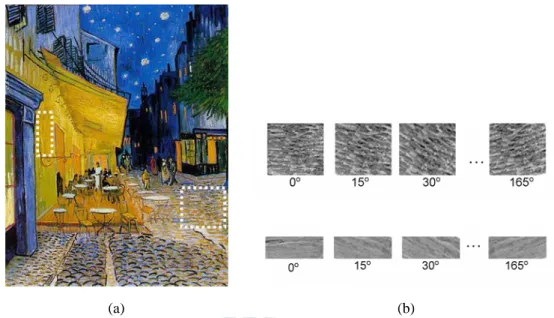
a. User select sample textures manually: User can select some sample textures form example painting, as Figure 3.4 exhibits, and the white dotted-line oblong is the selected area. The sample texture is the area where user thinks the stroke inside this area most stands for the style of this painting. We then compute the average direction each sample texture by luminance gradient, as equation 3.10 and 3.11 shows:
x f Gx ∂ ∂ = , y f Gy ∂ ∂ = (3.10) dir(pi) = tan-1( x y G G ) (3.11)
The average direction represents the stroke direction of this sample texture, but we need strokes with different directions to fit the variation of object
contour. So we duplicate twelve different rotated copies of each sample texture,
o
i 15× , i= 0, 1, ...11, as the Figure 3.4 shows. These duplicated copies will be
used in latter texture synthesis step. The average luminance of sample texture is computed by equation 3.12 N p L L N i i ave
∑
= = 1 ) ( (3.12)(a) (b) Figure 3.4 The illustration of one-pass texture synthesis. (a) Chosen sample textures from the
example painting. (b) The sample textures are duplicated 12 copies, each copy is rotated by 15o.
b. Decompose the projected image into regular cells: the projected image is decomposed into many regular cells. The cell is synthesis unit in the projected image, and the cell size is variable, range from 4×4 to 32×32. For each cell, we compute the average direction of it. The average direction of cell represents the surface undulation of 3D model because it is computed by the direction field. The detail of direction field is explained in subsection 3.3.3. We also compute the cell’s average luminance, which is used to find a proper sample texture during the next texture synthesis process.
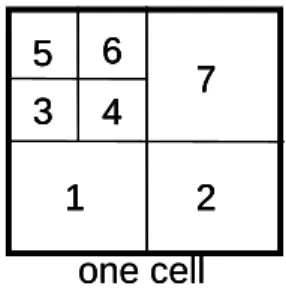
Figure 3.5 The cell division example. Cell will be divided into four subcell if the direction is inconsistent. The black arrows are some samples of direction of each pixels and the red arrow is the average direction of the subcell.
We compare each pixel direction with the mean direction within one cell. If the difference between pixel direction and average direction exceed a threshold, the cell is divided into four subcells. This approach has the advantage that the
cell does not need to compare directions of pixel with each other, and can quickly be divided if the directions are chaos. The cell is divided until the direction of pixels are similar to each other or the cell size is 4×4. Figure 3.5 displays the example of cell division. The average direction of cell/ subcell is used to find the orientation of object in projected image, so the stroke can synthesized according to the orientation of object. Thus the stroke will seem more natural and vivid in projected image, like the real stroke drawn by a painter.
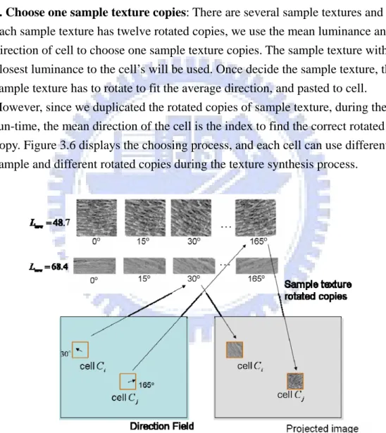
c. Choose one sample texture copies: There are several sample textures and each sample texture has twelve rotated copies, we use the mean luminance and direction of cell to choose one sample texture copies. The sample texture with closest luminance to the cell’s will be used. Once decide the sample texture, the sample texture has to rotate to fit the average direction, and pasted to cell. However, since we duplicated the rotated copies of sample texture, during the run-time, the mean direction of the cell is the index to find the correct rotated copy. Figure 3.6 displays the choosing process, and each cell can use different sample and different rotated copies during the texture synthesis process.
Figure 3.6 The example to choose sample texture. The cell direction comes from the direction field within the area of the cell. The direction could decide which sample texture rotated copies would be pasted to the cell.
scan line order, from the left to right, bottom to top. If the cell is divided as Figure 3.5, then the synthesized order is the shown in Figure 3.7:
one cell 1 2 3 4 5 6 7 one cell 1 2 3 4 5 6 7 1 2 3 4 5 6 7
Figure 3.7 Synthesis order. The example of texture synthesis. Take the cell in Figure3.5 as example. The cell is divided into 7 subcells, and the synthesis order is follow the number in the picture.
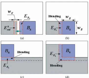
Since the sample texture which used as source in texture synthesis has decided, and then we have to search through the sample texture to find a proper texture patch, which is a square area with same size as the target cell/subcell, and will be pasted on the target area. When synthesized texture to one cell, we have to find a best-matching texture patch with the same size as the target cell/subcell from sample texture, i.e. the boundary distance between boundary zoneEBkand
k out
E
is minimal, as Figure3.8 shows. The gray area is the already synthesized cell and the blue area is the current target cell. In our application, we use 4 pixel width boundary to find the best-matching texture patch. Equation 3.13 is the distance function to compute the boundary error between target cell neighbors and the texture patch:
2 / 1 1 2 ] ) ( 1 [ ) , (
∑
= − = A i i out i B k out B L L A E E d k k (3.13)where A is the number of pixels in the boundary zone, and
i Bk L and i out L is the
luminance value of the ith pixel in the boundary zoneEBkand
k out
E
, respectively. Figure 3.8(b)(c)(d) are the four possible cases for boundary zone. The
overlapping boundary zone has to blending to eliminate the discontinuousness among cell boundaries.
Figure 3.8 The three conditions of boundary area. (a) The boundary error between
k out
E
and EBkhas to be mineralized. The gray area is already synthesized area,
and the blue area is current target cell. (b)(c)(d) are three situations of boundary. [LLX+2000]
e. Copy the texture and paste to the cell: after find the best-match cell, the texture of the sample texture are copied to the cell. The user can copy the full color channel, i.e. the L*a*b* color channel, or only the L* channel. In our application, only the luminance channel of the projected image is changed by that of the sample texture.
3.3.2 Two-Pass Texture Synthesis Framework
Generally, there are at least two steps to complete one painting, and our two-pass texture synthesis framework aims to simulate the two-pass procedure of drawing. The first step in procedure is sketching and applying a based layer on the canvas. The base layer provides the fundamental texture and color of the painting. In the second step, the artist shades the painting more concretely upon the base layer emphasizing the important features and the characteristics of objects which the painter wants to express.
Following this idea, we propose the two-pass texture synthesis framework. The first pass is called background pass which is used to emphasis the darker parts in the
projected image. The texture synthesis process in the background pass is the same as one-pass process, except for two things. The first thing is that the cell size is fixed in background pass. The result of the background pass is shown in the area with low luminance, i.e. the dark area in the projected image. Because the background pass usually shows in the area where the luminance is low and the viewer many not notice, so the strokes in this layer need not to be very smooth. So the biggest cell size is subtle enough to capture the feature of object for background pass, and accelerate the texture synthesis. Another advantage of big cell size is that the structure of stroke can be preserved much better.
(a) (b) Figure 3.9 Comparison of the two passes. (a) The background pass result and (b) The
foreground pass result.
The second pass is called foreground pass, which aims to emphasize the brighter part in synthesized image and synthesize the stroke with various direction. In
foreground pass, the synthesized image is also decomposed into regular cells, but the cells may be divided into subcells according to the directions of pixels in cells, as the explained in section 3.3.1. The stroke direction within a cell is identical. If we want to vary the stroke direction; we have to divide the cell. Because of the smaller cell size, the stroke can delineate the object in projected image more clearly, and variation of luminance can also be strengthened. Figure 3.9 show the result of only background pass and only foreground pass.
These two passes will generate two result luminance channels, and we combine the result by equation 3.10:
tex tex back L p L = ( )−μ tex tex fore L p L = ( )−μ (3.10)
img L = α /100 img back fore final L L L =κ( ×α+ ×(1−α))+μ
The subscript tex means the chosen sample texture, and img means the original projected image. Theα value is used to control the proportion of background pass result and foreground pass result. If the luminance in projected image is low, the background pass result will dominate the final luminance; otherwise if the
luminance is high, the foreground pass will be shown obviously. Figure 3.10 shows the result of one-pass and two-pass texture synthesis result.
(a) (b) Figure 3.10 The comparison of one-pass and two-pass framework. (a) The
one-pass rendering result. (b) The two-pass rendering result.
3.3.3 Direction Field
In this section, we explain how the direction filed is generated, and the difference of our direction field from that of the previous work of Bin Wang et al.. The direction field of Bin Wang et al. work is computed by media axis and Euclidean distance. They use color segmentation to divide an image into several different areas. We find the media axis for each area and compute the direction of the pixels in the area by Euclidean distance. However, the information of the direction field, which lacks the 3D informa -tion of objected in image, may be incorrect under some circumstances, because it cannot convey the bulge and hollow of object surface. For example, the direction field of a sphere in the photo may be circular, and the result of texture synthesis may make the sphere flat. For example, the direction filed of surface of a
sphere should be specified with horizontal vectors, but the method of Bin Wang et al. will generate circular direction, as Figure3.11 shows. Then the user will feel the sphere as a flat plane because of the incorrect direction field.
To resolve this problem, we use the tangent vector in our 3D model surface to compute the direction field. First, we compute the tangent vector of each triangle on the 3D model surface. Then we project the tangent vectors to a 2D image, which we use as the direction field. The surface tangent vector fields are an essential
ingredient in controlling surface appearance for many applications, such as NPR and texture synthesis. Hertzmann and Zorin pointed out some important properties of direction field which are used in illustration application: the direction field has to be continuous and follow the principal curvature direction [HZ00].
The first step is setting an initial tangential vector for each triangle of the model surface. In many previous application of generating tangential vectors, the user has to specify the initial vectors at certain key point [PHW+01][ HZ01]. Because we want to generate the direction field automatically, we initialize the mesh with a constant vector. An arbitrary vector, for example up vector [0, 1, 0], is projected onto the face of mesh. The tangential vector of each face is the cross product of the projected vector and the face normal.
After the initialization, a simple tangent field has been created, but the field is not continuous. To smooth out the tangent field, the tangential vector of each face is iteratively averaged with its three adjacent faces. Thought the averaging can be process many times to generate a smoothed result, the singularity of tangent field may still exist. The face clustering step is used to eliminate the singularity of the direction field.
The face clustering is computed by the method proposed by Garland et al.
(a) (b) (c) Figure 3.11 The difference of direction field of Wang et al. and our work. (a) The 3D sphere.
(b) The direction in the direction field of Wang et al. work. (b) The direction in the direction field of our work, the direction can present the surface curvature.
group owns the triangles with similar orientations, and the average tangential vector of these triangles is then assigned as the tangential vector of the group.
(a) (b)
(c)
Figure 3.12 The procedure of direction field. (a) The initialization of mesh (b) The cluster result (c) The tangential vectors of the surface after the averaging.
We average the tangential vectors among the groups instead of the faces of mesh. Each group averages its tangential vectors with neighbor groups iteratively as well. Finally, the tangential vector of the group is reprojected back to the triangles which in this group. Because the face with singularity must belong to one of the groups, and the reproject step will assign the tangential vector of the face, thus the face with singularity will have tangential vector too. The Figure 3.12 shows the result of each
step. θ Z Y X view plane θ Z Y X view plane
Figure 3.13 The method to project tangential vector to direction field. The tangential vectors are projected to the view plane, and the angle between the projected vector and the horizontal axis is the stored in the direction field.
The final step is projecting the tangent field of the mesh to the 2D image, which is the direction field. Instead of storing the direction as vector representation, we use the angle related to the x-axis as the direction. Figure3.13 illustrates the projecting process. The 3D model is drawn on the view plane, and the tangential vectors are also projected to view plane. The projected tangential vectors in the view plane are represented by their angleθ related to horizontal axis. The angle value is saved in color channel for each pixel in the image, thus the 2D direction field is colored with red, the first color channel. Figure 3.14 is the result direction field.
(a) (b) Figure 3.14 The direction field result. (a) The tangent vectors of the mesh (b) the
2D direction field.
3.4 Composite Projected Image into Example Painting
The projected image has to be pasted on to the example painting in the position where the user want to set the 3D object in. The Figure 3.15 (a) shows the position of 3D model in the painting. There are two areas in projected image: one is the object area, and the other is the non-object area, which is the black area in Figure 3.15 (b). The non-object area is transparent so the user only sees the object in the example painting. Then the projected image is pasted on the position where the user is put the 3D model in the painting. Figure 3.15(c) is the final result.
(a) (b) (c) Figure 3.15 The composition example. (a) The 3D model in the painting (b) the alpha map of projected image, the
4
C H A P T E R 4
Result
In this chapter we present several results synthesized by our system. All images are rendered using the OpenGL API. The hardware platform is a Windows PC with AMD Athlon 64 3000+ processor and 512Mbytes main memory. The graphics card is an NVidia GeForce6800 with the 8x AGP interface. We first show the result of the automatic color transfer of our system. Then the improvement of direction field is shown. Finally, the results of texture transfer and the projected image immersing into the painting are demonstrated in session 4.2.4.1 Result of color transfer and direction field
We first compare our color transfer result with the result of previous works.
Figure4.1(c) is the color transfer result of previous work [RAG+01]. In the work of Reinhard et al, a user can map the color between the reference image and the target photo manually. For example, the sky above the church is mapped to the deep blue sky in the painting, and the building is mapped to the wall of coffee shop. In our system, the mapping does not require the user assistance and pixel colors been classified into basic color categories automatically. In Figure 4.1(d), we can find that the pixel colors are transferred to proper color tone. For example, the blue jean of the standing man is still blue after the color transfer. The mean color of the reference image is yellowish color, so the result seems as if it is a result of filtering the input image by a yellowish filter.
(a) (b)
(c) (d)
Figure 4.1 The comparison of the color transfer. (a) reference painting (b) target photo (c) Result of [RAG+01] (d) Result of our method.
Although the convert of Reinhard et al. seems better, it needs the user manual control the color mapping between reference painting and input photo. In our method, the color mapping is automatic by using the Basic Color Categories. Figure 4.2 shows the effect of color transfer in our system. Without the color transfer, the object would still maintain its original color. This make the object visually incompatible with the example painting. On the other hand, after color transfer, the color used in object will like the color scheme of the example painting.
(a) (b) Figure 4.2 We put one cat model into the painting in the right bottom corner. (a) With
color transfer, the object could much immerse into the example painting. (b) Without color transfer, the object would seem incompatible with the example painting.
Figure 4.3 represents the effect of our direction field. The tangential vectors of the cat model is show in Figure4.3(a). Figure4.3(b) is a 2D direction field generated by projecting the tangential vectors on the 3D model surface to the view plane. We could see that the stroke is synthesized following the direction of direction field, as a painter to draw one object. The stroke direction near the head of cat is different from the direction of body. Otherwise, Figure4.3 (b) is the result without direction field, and the default direction is horizontal. Some features of cat model are lost, for example the ear and head seems flat without the direction field.
(c) (d) Figure 4.3 Comparison of the results with and without the direction field. (a) The tangential
vector of 3D model surface, the blue lines represent the vectors. (b)The 2D direction map from the 3D model surface projected. (c)The result with direction would have difference stroke direction. (b) The result without direction field seems flat.
4.2 The result of our system
Figure4.4 compare the result of two pass texture synthesis and one pass texture synthesis. The result of the one-pass texture synthesis appears much flat than the two-pass texture synthesis. Because the background pass use fixed patch size during the texture synthesis, it can preserve the structure of stroke much better than the foreground pass. The one-pass texture synthesis is absence of the texture which comes from the background pass, so that it seems much smooth and flat than the two-pass texture synthesis.
(a) (b) Figure 4.4 The effect of two-pass texture synthesis. (a) Result of one-pass texture
Figure 4.5 is a result of an oil painting and an irregular geometry object. The example painting is an abstract style oil painting and the boundaries of objects in it are obvious. We put a model with similar shape of objects in the example painting, so that the model could immerse into the painting easily. The user selects two
sample textures with different strokes. Figure 4.5(a) is the original example painting, with the sample textures (the white dotted-line square represent the areas which user selected). The object we put into the example painting is shown in Figure 4.5(b). Object is white, and we add one light to express the shading of the object. In Figure 4.5(c), the object appears in the bottom left corner of the example painting. We could see the object immerse into the painting well.
(a)
(b) (c)
Figure 4.5 (a) The example painting. The dotted-line square is the sample textures. (b) The object we put into the painting (the color has been transformed). (c) The final result.
Figure 4.6 is another result of our system. The object we put into the painting is a Cessna airplane. Figure 4.6(b) shows the original 3D object and its projected image after style transfer by our system . Then the project image is rendering with the example painting. The airplane has similar stroke and color scheme of example painting, immersing into the painting smoothly.
(a) (b)
(c)
Figure 4.6 (a) The example painting (b) The Cessna airplane model(top) and the image have the same style of the example painting(bottom) (c) The final result
Figure 4.7 shows water color painting example. We still put a Cessna airplane model into the example painting. The color of the projected image of the Cessna airplane has been changed the tone of airplane became gray. We can see that the style transfer algorithm of our system work well for water color painting.
(a)
(b)
5
C H A P T E R 5
Conclusion
5.1 Summary
We present a patch-based texture synthesis framework to accomplish our goal to immerse a 3D object into a 2D example painting. We tackle the problem of style transfer from the example painting by texture synthesis and color transfer techniques. To transfer the style of the example painting to the projected image of the 3D object, we use color and stroke as two main features of our system. The color scheme of the example painting is first analyzed by classifying the pixel color into 11 basic color categories. During the run time, the pixel color of the projected image is transferred in order to have similar color tone of the example painting.
After color transfer, we synthesize the stroke of the sample textures, which are selected by users from the example painting to be used as the source of texture. We propose a two-pass texture synthesis framework to transfer the stroke of sample textures onto the projected image. The strokes are synthesized with different directions according to the direction field. The direction field is computed by projecting the tangential vector of the 3D mesh surface to the view plane and computing the angle between project tangential vectors and horizontal line for each pixel, and store the angel value in direction field. With the direction field, the strokes will seem to be synthesized along the curved surface of the 3D model surface. Our system could transfer the style of the example painting well and immerse the 3D object into a painting seamlessly.
5.2 Future Work
In most paintings, a painter would use the shadow to emphasize the depth of space and make the painting more reality-looking. Besides shadow, it is also important to express the objects light and dark part. However, our system does not handle the shadow and lighting of objects because it is very hard to detect the position and intensity of the light source in the painting. In some image-based rendering
application, a user could use a series of photographs to compute the position of the light source. But in the painting, the light source is not very consistence in every part of the painting because the painter would change lighting in order to increase the beauty of the painting. Though it is hard to detect the correct lighting in the painting, we could offer a initial guess of light source and let the user change the light source freely.
Perspective view is important for immersing an object which wants to immerse into the painting. If the object does fit the perspective view of the painting, it would seem an excrescent in the painting. But in the painting, the painter would combine several different views in one painting. To compute the perspective view of painting precisely is very difficult. In our system, we offer an interface that user could zoom in or zoom out the object liberally. To prove the interface, we could first compute an initial guess of the perspective view of painting, and scale the objects according to the initial guessing. Then user could adjust the object by the control interface. Because we did not work on the boundary blending, the silhouette is shape in our system. However, using alpha blending is not a good method to smooth the boundary between object and the painting. Painters usually draw lines to describe the boundary of the object, so the shape of object would be definite, but not discontinues. It is desirable to depict the object by the same stroke of the example painting so the object would not separate from the painting because the shape boundary.
6
Bibliography
[Ash01] M. Ashikhmin. Synthesizing Natural Textures. In Proceedings of the 2001 Symposium Interatcive 3D Graphics, pp.217-226, 2001.
[BK69] B. Berlin, P. Kay. Basic Color Terms: Their Universality and Evolution. University of California Press. 1969.
[Bon1997] J.S.D. Bonet. Multiresolution Sampling Procedure for Analysis and Synthesis of Texture Images. In Proceedings of SIGGRAPH 1997, pp. 361-368, 1997.
[CGZ+05] Yung.Y. Chuang, Dan. B Goldman, Ke.C Zheng, Brian Curless, David H. Salesin, Richard Szelisk. Animating Pictures with Stochastic Motion Textures. In Proceedings of ACM SIGGRAPH 2005, 24(3): pp.853~860, July 2005.
[CSU+04] Y. Chang, S. Saito, K. Uchikawa, and M. Nakajima. Example-based color stylization based on categorical perception. In Proceedings of the First Symposium on Applied Percepton in Graphics and Visualization, pp.91~98, 2004.
[EF01] Alexei A. Efros, Willian T. Freeman. Image Quilting for Texture Synthesis and Transfer. In Proceeding of SIGGRAPH 2001, pp341-346, 2001.
[EL03] A.Efros and T. Leung. Texture Synthesis by Non-Parametric Sampling. In Proceedings of IEEE Int’l Conference Computer Vision (ICCV’ 99), pp. 1033-1038, 1999.
[EPW+00] Alex Eilhauer, Alice Pritikin, Dylan Weed, and Steven J. Gorther. Combineing Textures and Pictures with Specialized Texture Synthesis. 2000.
http://www.people.fas.harvard.edu/!pritikin/cs/graphics/
[FBS05] Jan Fischer, Dirk Bartz, Wolfgang Straßer. Stylized Augmented Reality for Improved Immersion. In Proceedings of IEEE Virtual Reality Conference 2005, pp.195-202, 2005.
[Fai1997] Fairchild, M.D. Color Appearance Model. Addison-Wesley. 1997.
[GCS02] Artistic Vision: Painterly Rendering Using Computer Vision Techniques. In Proceeding of Int’l Symp. Non-Photorealistic Animation and Rendering (NPAR 2002), 2002.
[GWH01] Michael Garland, Andrew Willmott, Paul S. Heckbert. Hierarchical Face Clustering on Polygonal Surfaces. In Proceedings of the 2001 symposium on Interactive 3D graphics, pp.49-58, 2001.
[Har2001] P. Harrison. A Non-Hierarchical Procedure for Re-Synthesis of Complex Textures. In Proceedinf of Int’l Conf. in Central Europe Computer Graphics an Visualization (WSCG 2001) pp. 190-197, 2001.
[HB1995] D.J. Heeger and J.R. Bergen. Pyramid Based Texture Analysis/Synthesis. In Proceedings of ACM SIGGRAPH 1995, pp. 229-238, 1995.
[HJO+01] Aaron Hertzmann, Charles E. Jacobs, Nuria Oliver, Brian Curless, David H. Salesin. Image Analogies. In Proceeding of ACM SIGGRAPH 2001, 2001.
[HS04] Michael Haller, Daniel Sperl. Real-Time Painterly Rendering for MR Applications. In Graphite, International Conference on Computer Graphics and Interactive Techniques in Australasia and Southeast Asia. pp.189-194, 2004.
[HZ00] Aaron Hertzmann, Denis Zorin. Illustrating Smooth Surface. In Proceeding of ACM SIGGRAPH 2000, pp.517-526.
[HZ01] Aaron Hertzmann, Denis Zorin. Illustrating smooth surfaces. In ACM Transactions on Graphics (Siggraph 2000), pp.517-526, 2001.
[LLW04] A.Levin, D.Lischinski, Y.Weiss. Colorization using optimization. ACM Transactions on Graphics, 23( 3): pp.689–694, 2004.
[LXG+01]L. Liang, C. Liu, Y.-Q. Xu, B. Gou, and H.-Y. Shum. Real-Time Texture Synthesis by Patch-Based Sampling. In ACM Transaction on Graphics, 20(3): pp. 127-150, 2001.
[PFH00] E. Praun, A. Finkelstein, and H. Hoppe. Lapped Textures. In Proceedings of ACM SIGGRAPH 2000, pp. 465-470, 2000.
[PHW+01] Emil Praun, Hugues Hoppe, Matthew Webb, Adam Finkelstein. Real-Time Hatching. In ACM Transactions on Graphics (Siggraph 2001), pp.581-586(21), 2001.
[RAG+01] E. Reinhard, M.Ashikhmin, B.Gooch, P.Shirley. Color transfer between images. In IEEE Computer Graphics and Applications, pp34-41, vol.21, 2001.
[RLC+06] Lincoln Ritter, Wilmot Li, Brian Curless, Maneesh Agrawala, David Salesin. Painting With Texture. In Eurographics Symposium on Rendering (2006)
[SCA+02 ]C. Soler, M.-P. Cani, and A. Angelidis, Hierarchical Pattern Mapping. In ACM Transactions on Graphics (Siggraph 2002), 21(3): pp. 673-680, 2002.
[Tur01] G. Turk. Texture Synthesis on Surface. In Proceedings of ACM SIGGRAPH 2001, pp. 347-354, 2001.
[TZL+02] X. Tong, J. Zhang, L. Liu, X. Wang, B. Guo, and H.-Y. Shum. Synthesis of Bidirectional Texture Functions on Arbitrary Surfaces. In ACM Transaction on Graphics (SIGGRAPH 2002), 21(3):pp.665-675, 2002.
[WAM02] Tomihisa Welsh, Michael Ashikhmin, Klaus Mueller. Transferring Color to Greyscale Image. ACM Transactions on Graphics, 21(3):pp277-280, 2002.
[WL00] L.-Y. Wei and M. Levoy. Fast Texture Synthesis Using Tree Structured Vector Quantization. In Proceedinf of ACM SIGGRAPH 2000, pp. 479-488, 2000.
[WWY+04] Bin Wang, Wenping Wang, Huaiping Yang, Jiaguang Sun. Efficient Example-Based Painting and Synthesis of 2D Directional Texture. In IEEE Transactions Visualization and Computer Graphics, 10(3):pp.266-277, 2004.
[XGS00] Y.-Q. Xu, B. Guo et and H.-Y. Shum. Chaos Mosaic: Fast and Memory Efficient Texture Synthesis. In Technical Report 32, Microsoft Research Asia, 2000.
![Figure 2.8 The result of work of Bin Wang et al.. (a) photo image (b) example painting (c) result synthesized image [WWY+04]](https://thumb-ap.123doks.com/thumbv2/9libinfo/8121255.165906/21.892.196.679.198.425/figure-result-wang-example-painting-result-synthesized-image.webp)
![Figure 3.3 Color circle. [CSU+04]](https://thumb-ap.123doks.com/thumbv2/9libinfo/8121255.165906/28.892.336.555.108.318/figure-color-circle-csu.webp)