國
立
交
通
大
學
電 子 工 程 系
碩
士
論
文
利用 Histogram 實現正交分頻多工系統資料輔助
時間訊號同步演算法
A NEW DATA-AIDED OFDM SYMBOL TIMING
SYNCHRONIZATION ALGORITHM BASED ON
HISTOGRAM PROCESSING
研 究 生:許勝毅
指導教授:桑梓賢 教授
利用 Histogram 實現正交分頻多工系統資料輔助
訊號時間同步演算法
A NEW DATA-AIDED OFDM SYMBOL TIMING
SYNCHRONIZATION ALGORITHM BASED ON
HISTOGRAM PROCESSING
研 究 生:許 勝 毅 Student:Hsu Sheng-Yi 指導教授:桑 梓 賢 Advisor:Sang Tzu-Hsien 國 立 交 通 大 學 電 子 工 程 學 系 碩 士 論 文 A ThesisSubmitted to Department of Electronics Engineering College of Electrical Engineering and Computer Science
National Chiao Tung University in partial Fulfillment of the Requirements
for the Degree of Master
in
Electronics Engineering June 2005
利用 Histogram 實現正交分頻多工系統資料輔助訊號時間同步演算法 學生:許勝毅 指導教授:桑梓賢 國立交通大學電子工程學系﹙研究所﹚碩士班 摘 要 一個新的資料協助符號同步演算法需要完成兩個目標:有更好的穩定度 和有效降低計算量。而一個直接的想法來自於訊號在時域的偏移會造成正 交分頻多工系統信號中的每個子載波在星座圖上的角度偏移,這也正是此 演算法的中心思想所在。再利用 histogram 的演算法從快速傅立葉轉換的 結果中用來尋找此時域偏移以節省複雜的計算量,其中也利用許多模擬來 驗證這個新的演算法的效率及可靠度。
A New Data-aided OFDM Symbol Timing Synchronization Algorithm Based on Histogram Processing
student:Hsu Sheng-yi Advisors:Dr. Sang Tzu-Hsien
Abstract
A new data-aided OFDM symbol timing synchronization method is developed with two goals in mind: to achieve robust performance and to reduce computational cost. It is the intuitive observation of the relationship between the symbol timing shift and the constellation rotation on each subcarrier of an OFDM symbol from which the new method is developed. A histogram-based algorithm is used to extract the timing shift information from the FFT output. Simulations are conducted to verify the effectiveness and robustness of this new algorithm.
誌 謝 本篇論文的完成要感謝許多人的幫助,首先要感謝的是我的指導教授 桑梓賢老師,研究過程中每當遇到瓶頸的時候,老師總是不厭其煩地幫助 學生去剖析問題,並解決問題,讓學生獲益匪淺。也要感謝 SPS 實驗室的 各位同學與學弟妹,在研究期間的幫忙與鼓勵。最後要感謝我的家人,許 賢德先生與蕭秀玉女士,在研究期間所給予的支持和關心。由於要感謝的 人實在太多了,若有遺漏,敬請見諒。
Contents
摘 要...I Abstract ... II 誌 謝... III Contents...IV Figure Contents ... V Chapter 1 Introduction ... 1Chapter 2 OFDM basics and optimal symbol timing ... 4
2.1 The introduction of OFDM ... 4
2.2 The basics of OFDM ... 5
2.2.1 The Classical structure of OFDM ... 5
2.1.2 The OFDM based on FFT ... 8
2.2 The features of OFDM ... 10
2.2.1 The Orthogonality of OFDM ... 10
2.2.2 Guard interval insertion ... 10
2.2.3 The Advantages and Drawbacks of The OFDM System ... 12
2.3 Timing Synchronization of OFDM System ... 12
2.3.1 Application Types of OFDM system... 12
2.3.2b Symbol synchronization... 20
Chapter 3 Proposed Algorithm... 24
3.1 Introduction of Histogram Operation... 24
3.2 The effect of symbol timing offset... 26
3.3 The Proposed Algorithm ... 27
Chapter 4 Simulation Results... 39
4.1 Description of Simulation Model... 39
4.2 Simulation Results ... 41
4.3 The Analysis of Differential Phase Offset (DPO)... 48
Chapter 5 Conclusion ... 51
Appendix ... 52
The Induction of the Probability Density Function of Differential Phase Offset (DPO) ... 52
Reference... 57
自 傳... 59
Figure Contents
Figure 2.1 Transceiver of a multicarrier system. ... 6Figure 2.2 The difference of the conventional and orthogonal systems8 Figure 2.3 Block diagram of OFDM system based on IFFT and FFT.. 9
Figure 2.5 MultiBand-OFDM preamble. ... 13
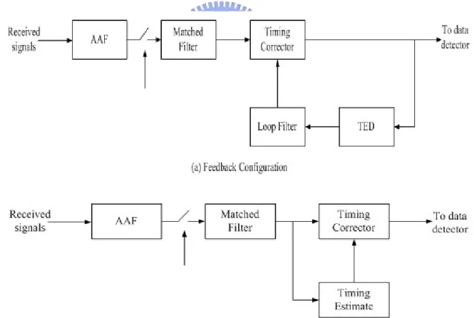
Figure 2.6 The basic blocks of (a) feedback and (b) feed-forward structures ... 15
Figure 2.7 Response of the double sliding window packet detection algorithm. ... 19
Figure 2.8 Double sliding window packet detection ... 19
Figure 2.9 Principal of symbol timing synchronization. (a) The original transmitted OFDM signals (b) The disturbed OFDM signals (c) safe/unsafe regions of symbol timing estimation... 22
Figure 2.10 Response of the symbol timing correlator... 23
Figure 3.1 An example of Histogram... 25
Figure 3.2 The symbol timing offset... 26
Figure 3.3 Block diagram of the receiver... 28
Figure 3.4 Inputs and outputs of IFFT and the OFDM signal. ... 31
Figure 3.5 Block diagram of the symbol timing offset estimator. ... 35
Figure 3.6 The diagram of the simple histogram operation... 36
Figure 3.7 The histogram of the DPOs through an AWGN channel with SNR=20dB. ... 38
Figure 4.1 The flow chart of the proposed algorithm ... 39
Figure 4.2 Estimate result due to the timing offset based on 16-bins histogram... 42
Figure 4.3 Estimate result due to the timing offset based on 32-bins
histogram... 42
Figure 4.4 Estimate result due to the timing offset based on 64-bins histogram... 43
Figure 4.5 Estimate result due to the timing offset based on 128-bins histogram... 43
Figure 4.6 Tracking performance of proposed algorithm (SNR: 10dB) based on 16-bins histogram (a) symbol timing recovery and (b) the histogram results. ... 44
Figure 4.7 Tracking performance of proposed algorithm (SNR: 10dB) based on 32-bins histogram (a) symbol timing recovery and (b) the histogram results ... 45
Figure 4.8 Tracking performance of proposed algorithm (SNR: 10dB) based on 64-bins histogram (a) symbol timing recovery and (b) the histogram results. ... 46
Figure 4.9 Tracking performance of proposed algorithm (SNR: 10dB) based on 128-bins histogram (a) symbol timing recovery and (b) the histogram results. ... 47
Figure 4.10 The movement of (x,y) given (z,w)... 49
Figure 4.11 Mean of different paths of Rayleigh fading channel. ... 49
Chapter 1 Introduction
Wireless communication plays an important role in our daily life. With lower price and more applications, wireless communication is getting popularized. In the future, folks will be eager to retire the miscellaneous cables and wires, and use wireless technologies to enjoy their home electric appliances. This phenomenon implies a quicker and more robust communication system is needed. The wireless communication system designers also sustain to design new modulated technologies and structures in order to transmit the increasing mounts of data. The OFDM (Orthogonal Frequency Division Multiplexing) technology is a kind of orthogonal multicarrier modulation technique. In accordance with the improvements in digital signal processing and VLSI technology, OFDM is being applied extensively to high data rate digital transmission, such as digital audio broadcasting, digital TV broadcasting, and wireless LANS.
In wireless environment, the transmitter usually transmits OFDM symbols in a packet-based fashion. The transmission, however, will be distorted by the unknown characteristics of the channel. As a result, the received OFDM symbols in a packet may not be recognizable.
substantial “leakage” from neighboring OFDM symbols exists. For this reason, the synchronization becomes an important step in the OFDM system. And the task of properly determining the start and end of each individual OFDM symbol and compensating any timing offset is called symbol timing synchronization, or symbol synchronization. Often a training signal sequence is used to facilitate this task. Currently, using initial timing synchronization preamble is the most prevalent means in burst applications.
Most of the existing methods of symbol timing synchronization fall into two major categories. The first is based on signal processing in frequency domain. This type of method first calculates the fast Fourier transform (FFT) of the received signal and the phase angle of each tone. The differences between the phase angles of each tone and a set of pre-determined reference phase angles are calculated. Then the phase differences are processed by, for example, fitting to a linear regression model. In this case, the timing offset can be estimated from the slope of the regression line. The second category is based on signal processing in time domain. Usually the received signal is correlated with a pre-determined reference time-domain signal.
Time domain methods often suffer significant performance degradation when strong co-channel interference or Gaussian noise is present. Properly designed frequency domain methods can achieve excellent performance. However, they often suffer from heavy computation required by processing the
phase angles obtained from the FFT of received signals. Also, due to their reliance on sophisticated signal processing algorithms, often they are not robust enough under conditions of severe noise. In this paper, a frequency domain method with low complexity for OFDM symbol timing synchronization is described. The remaining of this paper is organized as follows: Chapter 2 introduces the basics of the OFDM system. In chapter 3, the symbol timing synchronization algorithm based on histogram processing is presented. Simulation results are given in chapter 4 and the last chapter gives brief conclusions.
Chapter 2 OFDM basics and optimal symbol
timing
2.1 The introduction of OFDM
The basic principal of OFDM is to split a high-rate data stream into a number of lower rate streams that are transmitted simultaneously over a number of subcarriers, that is, using orthogonal subcarriers to achieve frequency multiplexing. A basic OFDM transceiver block diagram is listed below Fig. To mitigate the channel effects suffered during the transmission often a so-called circular prefix (CP) and/or suffix is introduced. These prefixes and/or suffixes are inserted between contiguous OFDM symbols and act as guardian intervals to reduce the possibility that waveforms interfere with each other, i.e. the data is transmitted after every signal adding cyclic prefix(CP), inserting pilots, and preambles used for synchronization. The pilots and preambles are regulated in the communication standard. In this chapter, the basics of OFDM, the task of timing synchronization and the optimal symbol timing are introduced.
2.2 The basics of OFDM
2.2.1 The Classical structure of OFDM
OFDM is a special case of multicarrier transmission, where a single datastream is transmitted over a number of lower rate subcarriers. Differ from the classical parallel data system and reduce the crosstalk between subcarriers, OFDM uses orthogonal subcarriers to achieve the transmission. The word orthogonal indicates that there is a precise mathematical relationship between the frequencies of the carriers in the system.
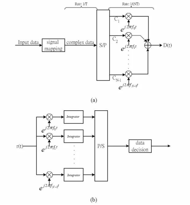
The figure 2.1 below is a basic transceiver of a multicarrier transmission system. The data after serial to parallel (S/P) carries to different subcarriers, i.e., if the original data rate is fs, the data rate will become fs/N after S/P, where N is the number of subcarriers. In this way, the OFDM system has a stronger capability to overcome the influence of intersymbol interference (ISI).
Figure 2.1 Transceiver of a multicarrier system.
(a) The transmitter of a multicarrier transmission system. (b) The receiver of a multicarrier transmission system.
The transmitting signal of each subcarrier is written as ( ) ( ) exp( 2 )
n n
D t =C t ⋅ j πf tn (2.1)
Then, the signal of transmitter is
1 0 ( ) N n( ) exp( 2 n ) n D t − C t j πf t = =
∑
⋅ . (2.2)Note that the subcarrier frequency must be chosen such that the signal of each subcarrier doesn’t interfere with one other. In a conventional multicarrier system, the total signal frequency band is divided into N non-overlappng frequency subchannels. Each subchannel is modulated with a separate symbol and then the
N subchannels are frequency-multiplexed. It seems good to avoid spectral
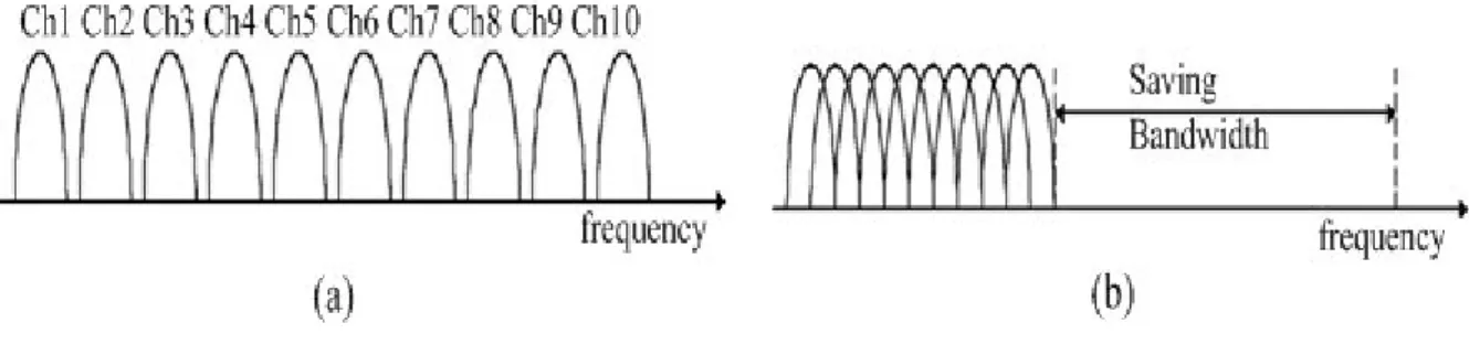
overlap of channels to eliminate interchannel interference. However, this leads to inefficient use of the available spectrum. To modify this side-effect and to save more bandwidth, the OFDM system arrange the carriers in an OFDM signal so that the sidebands of the individual carriers overlap and the signals are still received without adjacent carrier interference. To do this the carriers must be mathematically orthogonal. The figure 2.2 shows the difference of the conventional and the orthogonal situation. Besides, for generating N orthogonal subcarrers, the conventional multicarrier system calls for N oscillators. It is almost impossible to implement.
For the sake of implementation, Fast Fourier Transform (FFT) is used to substitute for oscillators.
Figure 2.2 The difference of the conventional and orthogonal systems (a) Conventional Multicarrier system. (b) orthogonal multicarrier system.
2.1.2 The OFDM based on FFT
Later on, how the OFDM system uses FFT to generate an OFDM symbol is showed. First, D(t) is sampled with sampling rate, 1/T. So, D(t) rewrites as
1 0 ( ) N n( ) exp( 2 n ) n D kT −C kT j π f kT = =
∑
⋅ . (2.3)Compare with the formula of inverse discrete time Fourier transformation (IDFT): 1 0 2 [ ] N [ ] exp( ) n j nk x k X n N π − = =
∑
⋅ . (2.4)A conclusion is that D(kT) = IDFT{Xn(kT)} if in place of f = n/NT. n As a result,
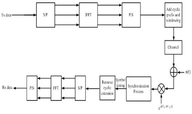
an OFDM signal is modulated by means of IFFT, likewise, demodulated by FFT. The figure 2.3 is a block diagram of OFDM system based on IFFT and FFT.
Figure 2.3 Block diagram of OFDM system based on IFFT and FFT.
From the figure above, the transmitter transforms a serial of high rate data into N low rate and parallel streams, first. Then every stream maps to individual modulated signal, such as QPSK, QAM, and so on. The N streams after modulation can be treated as signals in the frequency domain carry by N subcarriers. After the transform of IFFT, these streams are transferred into time domain and pass through P/S. At last, adding the guard interval (GI) to the serial of data then the transmitted data is ready. And the receiver only needs to reverse these functions to demodulate the received data.
2.2 The features of OFDM
2.2.1 The Orthogonality of OFDM
In this section, the reason why the OFDM signals are ofthogonal after the process of FFT is proved. Suppose there are N subcarriers, which are written as
( ) exp( 2 ), , 0,1, 2,3..., 1 k k k k t j f t f k N NT ϕ = π = = − . (2.5)
Check the inner product of i-th and j-th suncarriers:
2 1 2 1 * 2 2 2 1 exp( 2 ) exp( 2 ) ( ) exp( 2 ( ) )[1 exp( 2 ( ) )] exp( 2 ) 1 2 ( ) 0 ( ) . t t t t i j j t j t dt NT NT t t j i j j i j i j NT NT j t dt NT j i j NT T if i j if i j and t t NT π π π π π π ⋅ − − − − − = = − = ⎧ = ⎨ ≠ − = ⎩
∫
∫
1 t . (2.6)From the equations above, the subcarriers are orthogonal if the difference of any two subcarrers equals integer times of 1/NT. In this manner, one subcarrer does not interfere with other subcarriers.
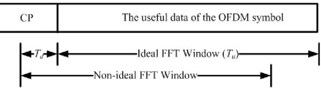
2.2.2 Guard interval insertion
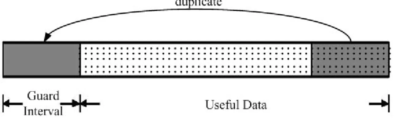
A guard interval is introduced for each OFDM symbol in order to avoid ISI caused by multipath channel. The guard time is chosen larger than the expected delay spread, such that multipath components from one symbol cannot interfere
with the next one. The GI could consist of no signal at all but in this case, however, the problem of intercarrier interference (ICI) would arise. ICI is crosstalk between different subcarriers, which means they are no longer orthogonal. To eliminate ICI, the OFDM symbol is cyclically extended in the GI just as showed in the Fig. 2.4. The meshed part in the figure represents the modulated useful data. The gray potion, head of the OFDM signal, is guard interval. It’s the duplication of the gray and meshed part in the modulated useful data. Hence, the lengths of the gray portion and the gray–mashed one are equal. The guard interval ensures that delayed replicas of the OFDM symbol always have an integer number of cycles within the FFT interval, as long as the delay is smaller than the guard time. With the help of cyclic prefix (CP), the orthogonality between the subcarriers does not be destroyed, however, only introduces a different phase shift for each subcarrier.
2.2.3 The Advantages and Drawbacks of The OFDM System
The OFDM transmission scheme has the following advantages: z OFDM provides high date rate.
z In relatively slow time-varying channels, it is possible to significantly enhance the capacity by adapting the data rate per subcarrier.
z Because the use of GI and a lower symbol rate, the OFDM system minimize the influence of ISI.
On the other hand, the Drawbacks of the OFDM system:
z OFDM calls for good synchronization to avoid the depredation on the orthogonality between subcarriers.
2.3 Timing Synchronization of OFDM System
2.3.1 Application Types of OFDM system
Synchronization is an essential task for any digital communication system. Without accurate synchronization algorithms, it is not possible to reliably receive the transmitted data. From the digital baseband algorithm design engineer's perspective, synchronization algorithms are the major design problem that has to be solved to build a successful product.
like WLAN. These two systems require different approaches to the synchronization problem. Broadcast systems transmit data continuously, so a typical receiver, such as European Digital Audio Broadcasting (DAB) or Digital Video Broadcasting (DVB) system, can spend a relatively long time to acquire the signal and then switch to tracking mode. On the other hand, packet switched systems typically have to use the so called "single-shot" synchronization; that is, the synchronization has to be acquired during a very short time after the start of the packet. This requirement comes from the packet switched nature of WLAN systems and also from the high data rates used. To achieve good system throughput, it is mandatory to keep the receiver training information overhead to the minimum. To facilitate the single-shot synchronization, current WLAN standards include a preamble, like the MultiBand-OFDM (MB-OFDM) preamble shown in Fig. 2.5. To avoid the abbreviation confusing, MB-OFDM is the posterity of IEEE 802.15.3a standard.
The OFDM signal makes most of the synchronization algorithms designed for single carrier systems unusable, thus the algorithm design problem has to be approached from the OFDM perspective. The frequency domain nature of OFDM also allows the effect of several synchronization errors to be explained with the aid of the properties of the DFT. Another main distinction with single carrier systems is that many of the OFDM synchronization functions can be performed either in time- or frequency-domain. This flexibility is not available in single carrier systems. But the trade-offs on how to perform the synchronization algorithms are usually either higher performance versus reduced computational complexity. Meanwhile, the synchronization algorithms are distinguished into data-aided (DA) and non-data-aided (NDA) depending on their operational styles. The data-aided synchronization algorithm usually uses the known data or symbols to estimate the timing, frequency or phase offset. Moreover, the DA algorithm inserts the pilots in the transmitted data or symbols to track the estimated results. Once the results go inaccurate, the synchronization algorithm could revise the estimated results to insure the receiver performs well. But in this way, the errors can’t vary too large to be out of the estimated range of the synchronization range. Hence, the positions of the pilots should well-defined, or the tracking is useless. The non-data-aided synchronization algorithms use the present decisions as the information to train the parameters requested by demodulator. The NDA algorithms usually use feedback and feed-forward
structures to compensate the timing. The feedback structure sends every estimated value back to the accumulator to maintain the estimated value lies in an acceptable range. Using this structure, however, should notice that the connections over the error signals, lowpass filters, and the feedback loop. On the other hand, the feed-forward structure uses the estimated result to compensate directly without feeding back to the results but how often the system estimates once depends on the system setup. The following figure shows the basic blocks of the two structures.
The following, all the synchronization algorithms mentioned are all data-aided manner and a new data-aided symbol timing synchronization algorithm is given in chapter 3.
2.3.2 The Task of Timing synchronization
There are two main tasks of the timing synchronization. One is the packet synchronization and the other is the symbol synchronization. In the following, the packet and the symbol synchronization are introduced.
In this paper, the focus is on the single-shot synchronization which is used for packet switched networks. Being prior to the core of this section, however, a main assumption made when designing the OFDM systems is that the channel impulse response does not change significantly during one data burst. This assumption is justified by the quite short time duration of transmitted packets and that the transmitter and receiver in most applications move very slowly relatively to each other. Under this assumption most of the synchronization for receivers is done during the preamble and need not be changed during the packet.
2.3.2a Packet synchronization
Packet detection is the task of finding an approximate estimate of the start of the preamble of an incoming data packet. Besides, it is the first synchronization
algorithm that is performed, so the rest of the synchronization process is dependent on the performance of packet detection. The simplest way for finding the start time of the incoming packet is to measure the received signal energy. If no packet is received, the received signal rn consists only of noise. But when the
packet comes, the received energy is increased by the signal component, thus the packet can be detected by the variation of the received energy. The decision variable mn is denoted as the received signal energy accumulated over some
window of length L to reduce sensitivity to large individual noise samples. The
mn can be written as 1 1 2 * 0 0 L L n n k n k n k k m − r r− − − r− = = =
∑
=∑
k . (2.7)It also can be written recursively as
2 2 1 1
n n n n L
m+ =m + r+ − r− +1 . (2.8)
This simple method suffers from a significant drawback; namely, the value of the threshold depends on the received signal energy. When the receiver is searching for an incoming packet, the received signal consists of only noise. The level of the noise power is generally unknown and can change when the receiver adjusts its Radio Frequency (RF) amplifier settings or if unwanted interferers go on and off in the same band as the desired system. When a wanted packet is incoming, its received signal strength depends on the power setting of the transmitter and on the total path loss from the transmitter to the receiver. All
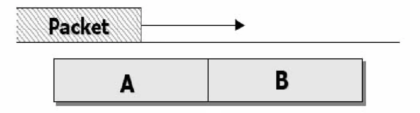
to decide when an incoming packet starts. A modified algorithm in the following is double sliding window packet detection. The double sliding window packet detection algorithm calculates two consecutive sliding windows of the received energy. The basic principle is to form the decision variable mn as a ratio of the total energy contained inside the two windows. Figure 2.2 shows the windows A and B and the response of mn to a received packet. In Figure 2.2, the A and B windows are considered stationary relative to the packet that slides over them to the right. It can be seen that when only noise is received the response is flat, since both windows contain ideally the same amount of noise energy. When the packet edge starts to cover the A window, the energy in the A window gets higher until the point where A is totally contained inside the start of the packet. This point is the peak of the triangle shaped mn and the position of the packet in Figure 2.2 corresponds to this sample index n. After this point B window starts to also collect signal energy, and when it is also completely inside the received packet, the response of mn is flat again. Thus the response of mn can be thought of as a differentiator, in that its value is large when the input energy level changes rapidly. The packet detection is declared when mn crosses over the
Figure 2.7 Response of the double sliding window packet detection algorithm. These steps mentioned above can be arranged as follow:
( )
1 * 0 1 1 2 * * 0 0 2 2 L n n k n k D k L L n n k D n k D n k D k k n n n c r r p r r r c m p − + + + = − − + + + + + + = = = = = =∑
∑
∑
. (2.9) (2.10) (2.11) where cn is the correlation of the A window and the B window, pn is theautocorrelation of the B window, and mn, the ratio of cn and pn, is the timing
2.3.2b Symbol synchronization
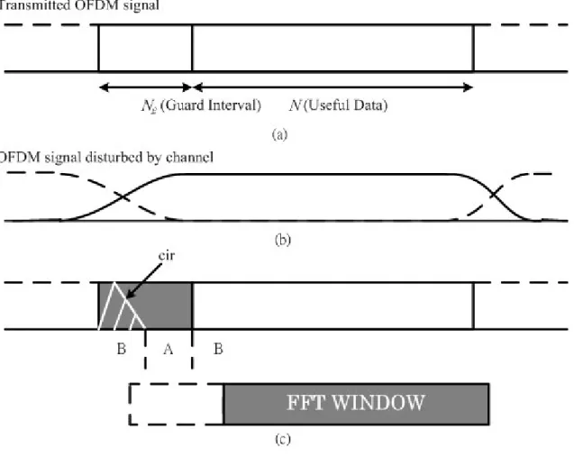
Symbol timing refers to the task of finding the precise moment of when individual OFDM symbols start and end. The symbol timing result defines the DFT window; i.e., the set of samples used to calculate DFT of each received OFDM symbol. The DFT result is then used to demodulate the subcarriers of the symbol. The approach to symbol timing is different for WLAN and broadcast OFDM systems. A WLAN receiver cannot afford to spend any time beyond the preamble to find the symbol timing, whereas a broadcast transmission receiver can spend several symbols to acquire an accurate symbol timing estimate. In Fig. 2.8, the first graph shows a transmitted OFDM signal, where Ng is the portion of
guard interval and N is the useful data, the second one presents the disturbed OFDM signal, and the last one defines which region is a proper symbol timing estimation. Due to the multipath propagation a part of the GI will be affected by reflections from the preceding symbol. The symbol timing synchronization must provide a proper estimated result that is influenced by one transmitted symbol only. In the case of a misalignment, there are two situations depicted in Fig. 2.8(c). As long as the start position of the FFT window is within region A, no ISI occurs. The only effect suffered by the subchannel symbols is a change in phase that increases with the subcarrier index. But the orthogonality between each subcarrier is not be destroyed. On the other hand, if the start position lies in
region B, the subcarriers not only have the influence of ISI but also the extra noise is introduced. It causes severely performance degradation resulted from the orthogonality is failed.
From fig. 2.8, it shows three consecutive OFDM symbols, their respective cyclic prefixes (CP), and the effect of symbol timing on the DFT window. The ideal timing for symbol 2 is shown as the ideal DFT window in Figure 2.10 (a). In this case the DFT window does not contain any samples from the CP, hence the maximum length of the channel impulse response (CIR) that does not cause intersymbol interference (ISI) is equal to the CP length. This is the maximum possible ISI free multipath length for an OFDM system.
As mentioned above, the OFDM synchronization functions can be performed in either time- or frequency-domain. The symbol synchronization algorithms are also presented in the both categories. In the time domain, it usually uses the correlation to determine the timing metric. And check the peak of the timing metric to estimate the symbol timing.
In a packet based receivers, the knowledge of preambles are available to them, which enables the receiver to use correlation based symbol timing algorithm. After the packet detector has provided an estimate of the start edge of the packet, the symbol timing algorithm refines the estimate to sample level precision. The refinement is performed by calculating the crosscorrelation of the received signal r and a known reference t ; for example, there are long and
short preambles defined in IEEE 802.11 standard. Then, the position of the end of the short training symbols or the start of the long training symbols is an observation to find the symbol timing estimate.
Figure 2.9 Principal of symbol timing synchronization. (a) The original transmitted OFDM signals (b) The disturbed OFDM signals (c) safe/unsafe
regions of symbol timing estimation
Equation 2.12 shows how to calculate the crosscorrelation.
1 * 0 ˆ arg maxn L n k k k n − r+ = =
∑
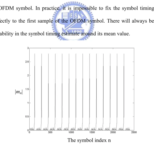
t . (2.12)The value of n that corresponds to maximum absolute value of the crosscorrelation is the symbol timing estimate. Figure 2.9 shows the output of the crosscorrelator that uses the preamble samples of the IEEE 802.15.3a standard as the reference signal. The simulation was run in Additive White Gaussian Noise (AWGN) channel with 10dB SNR. Each peak of |mn| shows a
symbol timing point.
The performance of the symbol timing algorithm directly influences the effective multipath tolerance of a OFDM system. An OFDM receiver achieves maximum multipath tolerance when symbol timing is fixed to the first sample of an OFDM symbol. In practice, it is impossible to fix the symbol timing point perfectly to the first sample of the OFDM symbol. There will always be some variability in the symbol timing estimate around its mean value.
|mn|
The symbol index n
Chapter 3 Proposed Algorithm
3.1 Introduction of Histogram Operation
In this paper, a new data-aided symbol timing synchronization is presented. Histogram operation performs an important role in the process of the algorithm. It directly affects the estimation result reliable or not, also reduces the cost of computational cost. So, the histogram is introduced beforehand.
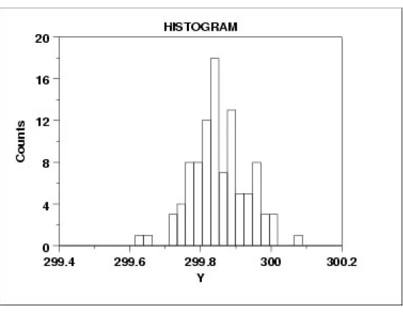
Histogram is a generally used expression in statistic. The purpose of a histogram is to graphically summarize the distribution of a data set, i.e., Histograms are used to summarize data graphically. A histogram divides the range of values in a data set into intervals. Over each interval is placed a block or rectangle whose area represents the percentage of data values in the interval. The histogram graphically shows the following:
1. center (i.e., the location) of the data; 2. spread (i.e., the scale) of the data; 3. skewness of the data;
4. presence of outliers; and
5. presence of multiple modes in the data.
These features provide strong indications of the proper distributional model for the data. The probability plot or a goodness-of-fit test can be used to verify the
distributional model. In the later, Kolmogorov-Smirnov goodness-of-fit test is used to determine the distributional model is right or not. A simple example (Fig 3.1) is listed below and shows the appearance of a number of common features revealed by histograms.
In the figure, the vertical axis represents “frequency”, i.e., counts for each bin. On the other hand, the horizontal axis stands for “response variable.”
Figure 3.1 An example of Histogram.
In this paper, we use the histogram operation to drive the distribution of differential phase offset (DPO). From the histogram of DPO, the symbol timing is determined. Besides, the different choices of bin numbers can be treated as a moving average result and the moving window size depends on the bin numbers.
3.2 The effect of symbol timing offset
There are frequency offset, phase offset, symbol timing offset and sampling timing offset that constitutes synchronization errors of OFDM systems. Among these, the symbol timing offset, Td, is the error factor concerned in this algorithm.
There exists an interesting relationship between symbol timing and the demodulated subcarrier phases. For this reason, the effect of the symbol timing offset is given in the following.
Figure 3.2 The symbol timing offset
Symbol timing recovery in the OFDM system is the function of detecting the start position of one OFDM symbol from the received signal. After this step, demodulation can be carried out by removing the guard interval and input the useful data interval into FFT block. The symbol timing offset is the difference between the correct symbol start position and the estimated symbol start position. Because of the FFT operation, this difference is reflected in the individual phase
of each subcarrier. The relationship between the phase of the k-th subcarrier and the symbol timing offset Td is given by [7]
2 d k u T k T φ = − π , (3.1)
where Tu is the interval of the useful data. From the relationship between the
phase rotation φk and the subcarrier index k, the symbol timing offset Td can be
estimated.
3.3 The Proposed Algorithm
The timing uncertainty often arises when using the time domain algorithms, except the more complicated ML ones, are used. This implies the ISI will be introduced if the estimated results of the time domain algorithms are directly applied. Often an ad hoc correction term is applied to achieve better results after the location of the peak correlation coefficient being determined. But the compensating rules are ad hoc as well and the optimal timing estimation is usually not obtained. Frequency domain algorithms, on the other hand, may avoid this problem. The receiver structure is listed below, Fig 3.3. In the figure, the receiver generates the received packet from the antenna first. After the S/P, the signals in the packet pass to the FFT directly. Then from the outputs of the FFT, the symbol timing offset estimator collects the information to estimate the symbol timing offset. The received data is also passed to the demodulation
Figure 3.3 Block diagram of the receiver.
Before going to the details of the algorithm, the OFDM signal model and the concept of differential phase offset (DPO) are introduced first, especially the DPO is taken as a metric that contains information of any misalignment of symbol timing, i.e., The DPO is the data used for determining the symbol timing offset. DPO is introduced first, and the OFDM signal model is followed.
For the convenience and distinguishing with all other phase terms talked in the algorithm, DPO is defined to represent the phase difference of two adjacent received subcarriers. Note that the phase of each received subcarrier has made some modification before generating DPOs. More delicate details are given in the following.
First, suppose there is a time domain transmitted signal x(t), then the pair of time domain signal x(t) and its FFT Xk is represented as:
( ) k k exp( k)
x t ⇔ X = A jϕ . (3.2)
Therefore, after the transmission, the received signal R(t) and its frequency domain signal can be expressed as:
( ) k kexp( k)
R t ⇔R =B jΨ . (3.3)
In the last two equations, Ak and
φ
k are the amplitude and the original phase of Xk respectively, likewise, Bk andΨ
k are the amplitude and the phase of Rkindividually. Because the phase After the phase
Ψ
k is modified by the phaseφ
k ,finally, DPO (denoted by
Δ
k) is the modified phase difference of theneighboring k-th and (k+1)-th subcarrier, i.e.,
1 1
( ) (
k k+ ϕk+ k ϕk)
∆ = Ψ − − Ψ − . (3.4)
The definition of DPO is stated above and the reason why DPOs could be used for determining the symbol timing will be given in the later. For now, the focus is changed to the signal model. Through this model, the core idea of the proposed algorithm is also introduced.
The OFDM signal is generated at baseband by taking the inverse fast Fourier transform (IFFT) of quadrature phase shift keyed (QPSK) subsymbols. The samples of the transmitted signal can be expressed as:
1 0 1 ( ) N n exp( 2 / ), g 1 n x k c j kn N N k N N
π
− = =∑
− ≤ ≤ − . (3.5)where cn is the modulated data with the phase
φ
k, N is the number of IFFTpoints, Ng is the number of guard samples, and n stands for the index of
subcarrier. All the parameters are all defined in the Fig 3.4. Meanwhile, at the receiver side, there exist impairments caused by carrier-frequency offset, sampling clock errors, and symbol timing offset. Usually, the frequency offset and timing errors are more dominant than the sampling clock inaccuracy.
Hence, in this paper, the symbol timing synchronization will be considered assuming a perfect sampling clock.
Then, suppose the channel is modeled with a timing delay (D) and a phase offset (θ), then it can be written as:
h( k )=exp( j ) ( kθ δ −D ). (3.6) Therefore, the received OFDM signal, r(k), through the equivalent channel, h(k), will be
( ) exp( ) ( )
r k = j s k Dθ − . (3.7)
To simplify the illustration of the algorithm, the noise term is ignored. As a result, the i-th received OFDM symbol will be
1 , 0 1 2 ( ( ) exp( ) N exp( ) i i n n ) j k D n r k j c N N π θ − = − =
∑
. (3.8)This received OFDM symbol will be passed to FFT directly. At the output, the symbol will be 1 , 0 2 ( ) exp( ) N i k i n j kn R r n N π − = =
∑
⋅ − . (3.9)Figure 3.4 Inputs and outputs of IFFT and the OFDM signal.
where k is a index of subcarrier, and i is a received symbol index. Carrying equation 3.8 r (ki ) into equation 3.9 Ri,k to replace r (ni ), then, the received OFDM
signal becomes
1 1
, ,
0 0
1 2 ( )
[exp( ) exp( )]exp( )
N N i k i l n l 2 j n D l j nk R j c N N N π θ − − = = − =
∑
∑
− π . (3.10)result, the received i-th OFDM symbol at k-th subcarrier can be expressed as , , 2 1 exp( ) exp( ) i k i k j kD R j c N N π θ − = ⋅ ⋅ . (3.11)
Until now, the definition of DPO and the system model are both introduced. The next step is the key player of proposed algorithm. How to generaet the DPOs from the received signals and why the proposed algorithm works are given in the following paragraph.
First, extract the phase of Ri,k out, denoted as
Ψ
k. Note the index i is omittedbecause the operations made in the following all in the same OFDM symbol, so only the index k of subcarrier need to taking into consideration. So, the phase of the i-th OFDM symbol at k-th subcarrier is
2 k k j kD N π θ − ϕ Ψ = + + . (3.12)
Carry the
Ψ
k to the definition of DPO, ∆ = Ψ −k ( k+1 ϕk+1) (− Ψ −k ϕk), then thecomputational result is 1 1 1 1 ( ) ( ) 2 ( 1) 2 [( ) ] [( ) ] 2 ( 1 ) 2 k k k k k k k k k D kD N N D k k D N N ϕ ϕ π π k θ ϕ ϕ θ ϕ ϕ π π + + + + ∆ = Ψ − − Ψ − − + − = + + − − + + − − + − − = = . (3.13)
On the other hand, there is an effect need to consider if the symbol timing doesn’t fetch the ideal FFT window, as mentioned in 3.2. Because of symbol timing effect induced by the non-ideal FFT window, the received i-th OFDM symbol at k-th subcarrier after FFT will be
, ,
2 2
exp( ) exp( ) exp( D)
i k i k j kD j kT 1 R j c N N N π π θ − − = ⋅ ⋅ ⋅ , (3.14)
where Td , normalized to sample based, is the symbol timing offset.
Follow same steps of generating DPO, the DPO will be
1 1 1 1 ( ) ( ) 2 ( 1) 2 ( 1) 2 2 [( ) ] [( ) ] 2 ( )( 1 ) 2 ( ) k k k k k D D k k k D D k D k T kD kT N N N N D T k k D T N N ϕ ϕ π π π π k θ ϕ ϕ θ ϕ ϕ π π + + + + ∆ = Ψ − − Ψ − − + − + − − = + + + − − + + + − − + + − − + = = (3.15) Hence, the timing offset introduced by D and Td can be estimated through the
DPOs as well.
Clearly, the information of symbol timing offset is encoded in the DPOs. Assuming there are N (indexed by n = 1 to N) subcarriers in an OFDM symbol, then there will be (N-1) DPOs (indexed by k = 1 to N-1) available for one OFDM symbol. From the relation between time and frequency domain, a delay/ahead in time domain will introduce a negative/positive phase in frequency domain. So, DPO is ranged from -π to π. But for the simplicity of histogram, DPO maps to the new range of 0 to 2π temporally. In this way, the histogram will be done by simple comparisons. Once the phase introduced by a timing delay is estimated, the result still needs to re-map to the range between -π and π while computing the value of time delay D.
phase angle and the correct phase of each tone is calculated, i.e., for each k, the difference (
Ψ
k-φ
k) is calculated. Note that since the calculation is done withmod 2π arithmetic, the result will be wrapped within the range of 0 to 2π. Then the DPO is calculated for k = 1 to N-1. This calculation is done with same operation, mod 2π arithmetic, so the result is between 0 and 2π as well. There are (N-1) DPOs calculated for one OFDM symbol, but the receiver is not restricted to use all of them for the purpose of symbol timing synchronization. A subset of the calculated DPOs may be used. Nor is the receiver restricted to use one OFDM symbol’s worth of data to estimate the symbol timing offset. More than one OFDM symbol can be used if conditions permit. For example, if K OFDM symbols and (N-1) DPOs per symbol are used, there will be K(N-1) DPOs to be processed. In this paper, only the case of one symbol (K = 1) is described for the sake of simplicity. The case of multiple symbols is a straightforward generalization that can be done easily. Next, the histogram of DPOs is obtained. After the interval from 0 to 2π is normalized to a new range from 0 to 2 -1N , this new interval, from 0 to 2 -1N , is divided into 2L bins. The key idea of the method is to fetch the first L bits of each normalized DPO to be the selector of a MUX and a DEMUX (Fig. 3.6). Each address of register, which is used for saving the current value to a corresponding bin, is treated as the lower boundary of each bin.
Figure 3.5 Block diagram of the symbol timing offset estimator.
The value stored in each register will be fetched and add 1 to the value, then the new value will be returned to the same register when a register is selected by a truncating DPOs. After all DPOs are checked, the histogram operation is done at the same time. The histogram of DPOs is further processed to determine the timing delay D. The peak of histogram, i.e., the bin which has the highest frequency, is chosen. Assume the peak occurs at the l-th bin. The l-th bin ranged
from ( 1) 2l L π − ⋅ to l 2 L π
⋅ , represents the possible values for D is from 1 (l )N
L
−
to ( )l N
L . Therefore, the estimation of can be chosen asn
0.5
(l )N
L
−
, i.e., the average of the possible values. Note the estimation of D will be (l 0.5 1 N
L
−
− ) if
the lower boundary of the l-th bin is greater than π. The reason why (l 0.5)
L
−
minuses 1 comes form the phase need to be wrapped between -π to 0. Once the symbol timing offset is estimated, the symbol timing synchronization can be easily achieved by adjusting the boundaries of each time domain OFDM symbol. A positive D means that the current boundaries are behind the correct boundaries and need to be moved ahead by D samples. Inversely, a negative D means the boundaries need to be delayed by D samples.
As an example, consider a linear-phase channel, whose impulse response is symmetric around , that is, n0 h n[ ]=h n[2 0−n],0≤ ≤n 2n0 and the corresponding FFT output is
0
exp( 2 / ),
k k
H =C ⋅ −j πkn N+β (3.16)
And the received signal after FFT is
0
exp( 2 / ).
k k k k
R =A C⋅ ⋅ −jφ − j πkn N+β . (3.17)
By the proposed algorithm, the DPO is 2 n0
N
π if no noise exists. At last, the
symbol timing estimation is n0.
Besides, a simple simulation is given here. Consider an OFDM system with a FFT window size is 50 transmits the signal through an AWGN channel with SNR = 20dB and the optimal delay of the channel is 25. From the context above, this delay will introduce a phase shift on each subcarrier of an OFDM symbol. From equation 3.13, the DPO should lie around -π( 2 (25)
50 )
π
−
= . Then, taking
these DPOs through a histogram operation. Figure 3.7 is the histogram result of the DPOs. This histogram is operated under 64 bins, i.e. the range from –π to π is divided into 64 subintervals. From the figure, the peak is occurred around -3.09. There are not only one bin containing all the DPOs because the presence of noise. So, the delay will be estimated at 25 ( 3.09 50
2π ×
The center of this container is -3.09 F re qu en cy Phase (radian)
Figure 3.7 The histogram of the DPOs through an AWGN channel with SNR=20dB. This histogram is divided into 64 bins.
The computation cost of the proposed algorithm, taking one complete OFDM signal with N subcarriers of the OFDM system into account, is 2N subtractions and N comparisons. It is better than the correlation method [1], which calls for 2N multiplications, N additions, and N subtractions. As for the computation amount of phase extraction is not counted here because the phase extraction operation is a task of demodulators in M-PSK OFDM systems.
Chapter 4 Simulation Results
4.1 Description of Simulation Model
In last chapter, the proposed algorithm is introduced. The figure below shows the ideal of the algorithm. After the packet detection, the received signal is passed through S/P to generate the parallel signal. After the processing of FFT, the signal will be transformed to the frequency domain. These signals in frequency domain can be used to generate DPOs. Then, DPOs are processed by the histogram operation. From the result of the histogram, the peak is used to determine the symbol timing.
Simulations have been run to evaluate the performance of the algorithm. The algorithm is applied to a model based on the IEEE 802.15.3a standard [4]. The OFDM system parameters used are 128 subcarriers, 128 point IFFT/FFT, a cyclic prefix of 32 samples and a guard interval of 5 samples. The value of a subcarrier frequency spacing is 4.125MHz (=528MHz/128) and a symbol time is 312.5ns. The 100 data subcarriers are modulated by QPSK and all channels are set to be 16 taps.
The channel is modeled in frequency-nonselective fading channels. Besides, the transmission path without line-of-sight (LOS) introduces an uncorrelated Rayleigh fading distortion to the corresponding transmitted signal. The uncorrelated Rayleigh fading distortion is often modeled as a complex Gaussian fading process:
[ ] [ ] * [ ] , 0 1
h n =a n + j b n ≤ ≤ −n L , (4.1)
where a[n] and b[n] are tow statistically independent real-valued baseband Gaussian waveforms. A channel is static in each simulation but changes from one simulation to another. And as mentioned in chapter 3, the sampling clock error is not considered here, i.e. the simulations are run assuming a perfect sampling clock.
4.2 Simulation Results
Figure 5.2 ~ Figure 5.5 shows the tracking of the proposed algorithm for input SNR = 10. The proposed algorithm is simulated with 16, 32, 64, 128 bins histogram. The timing offset (x-axis) means the timing chosen to set the FFT window when the packet detector is alarmed. Through the different inputs from different timing, the proposed algorithm is still functional on different bin numbers. From the curves in these figures, the estimated results based on a small-number-bins histogram are not as sensitive as a large number one. Also, the robustness of the proposed algorithm is also showed while a large-number-bins histogram is used. But it is obvious that the computation cost will be heavier if a larger number of bins is used.
In the figure 5.6 ~ 5.9, the tracking performance of proposed algorithm for input SNR = 10dB is presented. The OFDM symbol index (x-axis) stands for the preamble index of the IEEE 802.15.3a standard, as showed in figure 2.5. Packet synchronization sequence (the first column) is used for the coarse timing synchronization. There are 21 symbols used for the synchronization, on the other hand, it also means the synchronization should be done in 21 symbol time. From the simulations, the algorithm calls for 3 symbol time to achieve a stable timing result.
Timing offset -45 -40 -35 -30 -25 -20 -15 -10 -5 0 -35 -30 -25 -20 -15 -10 -5 0 E sti m ate re su lt
Figure 4.2 Estimate result due to the timing offset based on 16-bins histogram Timing offset -45 -40 -35 -30 -25 -20 -15 -10 -5 0 -35 -30 -25 -20 -15 -10 -5 0 E sti m ate re su lt
Timing offset -45 -40 -35 -30 -25 -20 -15 -10 -5 0 -35 -30 -25 -20 -15 -10 -5 0 E sti m ate re su lt
Figure 4.4 Estimate result due to the timing offset based on 64-bins histogram. Timing offset -45 -40 -35 -30 -25 -20 -15 -10 -5 0 -35 -30 -25 -20 -15 -10 -5 0 E sti m ate re su lt
(a) After compensation 1st estimated result F re qu en cy Phase (radian) (b)
Figure 4.6 Tracking performance of proposed algorithm (SNR: 10dB) based on 16-bins histogram (a) symbol timing recovery and (b) the histogram results.
(a)
1st estimated result After compensation
F re qu en cy Phase (radian) (b)
Figure 4.7 Tracking performance of proposed algorithm (SNR: 10dB) based on 32-bins histogram (a) symbol timing recovery and (b) the histogram results
(a) 1st estimated result After compensation F re qu en cy Phase (radian)
Figure 4.8 Tracking performance of proposed algorithm (SNR: 10dB) based on 64-bins histogram (a) symbol timing recovery and (b) the histogram results.
(a) After compensation 1st estimated result F re qu en cy
Figure 4.9 Tracking performance of proposed algorithm (SNR: 10dB) based on 128-bins histogram (a) symbol timing recovery and (b) the histogram results.
4.3 The Analysis of Differential Phase Offset (DPO)
As mentioned in the chapter 3, the DPO is treated as the metric to determine the symbol timing offset. In another words, DPO directly effects the performance of the algorithm. Besides, the histogram operation gives the mean value of DPOs. As a result, the probability density function (pdf) of DPO becomes what needs to take into consideration. But for arbitrary channels, it is difficult to analyze the behavior. We transform the question into a statistical one: Rayleigh fading channels to derive the behavior of DPOs.
The real part (X) and the image part (Y) of the k+1-th subcarriers and the real part (Z) and the image part (W) of the k-th subcarriers are treated as the random variables. The four random variables will give the covariance matrix and the joint pdf because the proposed algorithm is operated in frequency domain and FFT makes the k-th subcarrier and k+1-th subcarrier dependent. As the help of the joint pdf of X,Y, Z, and W, the conditional pdf of X and Y given Z and W, i.e., p(X,Y|Z,W), is derived. By the mean of the conditional pdf, the mean of DPO is πL/N, where L is the paths of multipath channel and N is the points of the FFT. The figure below shows the relationship between the mean of DPO and the paths of multipath. And the figure 4.11 tells the mean value of DPO when the length of multipath is given. The results are simulated at 128 points FFT.
Figure 4.10 The movement of (x,y) given (z,w)
By the joint pdf of X,Y, Z, and W again, the pdf of DPO is also derived. Figure 4.12 shows the theoretical pdf and the simulation results. With the deviation of the pdf of DPO, it gives the proposed algorithm a strong theoretical prediction and tells the reliability of the proposed algoritm.
Chapter 5 Conclusion
In this paper, the basics of the OFDM system are given and the time synchronization is also illustrated, especially the task of the symbol timing synchronization.
An algorithm based on histogram processing to solve the problem of symbol timing synchronization of OFDM system is described. The proposed algorithm is more robust for finding the timing without any ad hoc time shift instead of the traditional correlation methods. The algorithm also deals with the symbol timing offset, which has the degree of the phase rotation is proportional to subcarrier index. Besides, the proposed algorithm can also used to track the symbol timing by the pilots, which is inserted in the data interval, but the definition of DPO need to multiply a reciprocal of inter-pilot spacing.
Although the phase extraction costs heavy computational amount, it is not counted here because the phase extraction operation is a task of demodulators in M-PSK OFDM systems. In short, it is a strong candidate for timing synchronization need of OFDM systems using M-PSK modulation.
Appendix
The Induction of the Probability Density Function of
Differential Phase Offset (DPO)
Suppose Rayleigh fading channel in the time domain with L paths. As a result, it can be expressed as
[ ] [ ] * [ ] , 0 1
h n =a n + j b n ≤ ≤ −n L , (A.1)
where a[n] and b[n] are tow statistically independent real-valued baseband Gaussian waveforms with zero mean and the variance is σ2. Then, the FFT output of the h[n] at the k-th subcarrier is
1 0 1 0 1 0 2 [ ] exp( ) 2 2 ( [ ] * [ ]) (cos( ) *sin( )) 2 2 2 2
( [ ] cos( ) [ ] sin( )) *( [ ] sin( ) [ ] sin( )))
L k n L n L n j nk H h n N nk nk a n j b n j N N nk nk nk nk a n b n j b n a n N N N π π π π π π − = − = − = − = ⋅ = + ⋅ − = ⋅ + ⋅ + ⋅ − ⋅
∑
∑
∑
πN (A.2)Because DPO is the phase offset of the k-th subcarrier and the k+1-th one, the probability density function (pdf) must be involved in the relationship between two adjacent subcarriers. And with the highly correlated between the k-th subcarrier and the k+1-th one, we will conduct the pdf of DPO by the conditional pdf and the joint pdf. The conditional pdf is used for evaluating the
mean behavior of DPO and the joint pdf is used for deriving the pdf of DPO. For simplicity, the real part and the image of Hk part are defined as Z and W
individually. The real part and image part k+1-th subcarrier are denoted as X and
Y respectively. As a result, Z, W, X, and Y are defined as follow,
1 0 1 0 1 0 1 0 2 2 [ ] cos( ) [ ] sin( ) 2 2 [ ] cos( ) [ ] sin( ) 2 ( 1) 2 ( 1) [ ] cos( ) [ ] sin( ) 2 ( 1) 2 ( 1) [ ] cos( ) [ ] sin( ) L n L n L n L n nk nk Z a n b n N N nk nk W b n a n N N n k n k X a n b n N N n k n k Y b n a n N N π π π π π π π π − = − = − = − = = ⋅ + ⋅ = ⋅ − ⋅ + + = ⋅ + ⋅ + + = ⋅ − ⋅
∑
∑
∑
∑
, (A.3)Now, the focus is changed to the covariance of Z, W, X, and Y. After evaluating the correlation of Z, W, X, and Y pairwisely, the inverse covariance matrix is
1 1 2 2 2 0 0 1 1 2 2 2 0 0 1 1 2 2 2 0 0 1 1 2 2 2 0 0 2 2 0 cos( ) sin( ) 2 2 0 sin( ) 2 2 cos( ) sin( ) 0 2 2 sin( ) cos( ) 0 L L n n L L n n L L n n L L n n n n L N N n n L N K n n L N N n n L N N π π σ σ σ π π σ σ σ π π σ σ σ π π σ σ σ − − = = − − = = − − = = − − = = ⎡ − ⎤ ⎢ ⎥ ⎢ ⎥ ⎢ ⎥ ⎢ ⎥ ⎢ ⎥ = ⎢ ⎥ ⎢ ⎥ ⎢ ⎥ ⎢ ⎥ − ⎢ ⎥ ⎢ ⎥ ⎣ ⎦
∑
∑
∑
∑
∑
∑
∑
∑
cos( ) N , (A.4)Also for simplicity, denoting the combinations of the cos and sin as a and b individually: 2 2 1 2 0 1 2 2 cos( ) 2 sin( ) H L n L L n a N n b σ σ π σ π σ − = − = ⋅ = =
∑
∑
(A.5)Then, the determinant of K is
4 2 2
det( ) (K = σH −(a +b ))2 (A.6)
And the inverse of K is
2 4 2 2 4 2 2 4 2 2 2 4 2 2 4 2 2 4 2 2 1 2 4 2 2 4 2 2 4 2 2 2 4 2 2 4 2 2 4 2 2 0 0 0 0 H H H H H H H H H H H H H H H a b a b a b a b b a a b a b a b K a b a b a b a b b a a b a b a b σ σ σ σ σ σ σ σ σ σ σ σ σ σ σ − ⎡ − − ⎤ ⎢− + + − + + − + + ⎥ ⎢ ⎥ ⎢ − ⎥ ⎢ ⎥ − + + − + + − + + ⎢ ⎥ = ⎢ − ⎥ ⎢ ⎥ − + + − + + − + + ⎢ ⎥ ⎢ − − ⎥ ⎢ ⎥ ⎢− + + − + + − + + ⎥ ⎣ ⎦ H σ (A.7)
By the definition of multidimentional Gaussian distribution, the joint probability density function of random variable (r.v.) X,Y, Z, and W is
[
]
1 1/ 2 1 1 ( , , , ) exp( ) 2 (det( )) 2 x y p x y z w x y z w K z k w π − ⎡ ⎤ ⎢ ⎥ ⎢ ⎥ ⎡ ⎤ = − ⎣ ⎦ ⎢ ⎥ ⎢ ⎥ ⎣ ⎦ . (A.8)First, the exponential term in the conditional pdf of random variable X and Y given Z and W,i.e., p(x,y|z,w), is extracted out to evaluate the mean behavior of the DPO. 2 2 2 4 2 2 2 2 1 exp{ [( ) ( ) ]} 2 H H H az bw bz aw x y a b σ σ σ σ − + − − + − − − H . (A.9)
From (A.9), the center of (x,y) is not moving independently while the former subcarrier (z,w) is given. If (z,w) is given, then
2 2 ( , ) ( , ) H H az bw bz aw x y σ σ − + = . (A.10)
From (A.10), neglecting the coefficient the rotation matrix is a b b a − ⎡ ⎤ ⎢ ⎥ ⎣ ⎦. (A.11)
Because the integration of cosine is sine, a and b can be approximated as:
1 0 1 2 1 2 cos( ) sin( ) 2 1 2 sin( ) ( cos( ) 1) L n L n L N N n L N N 0 n π π π π − = − ≈ ⋅ ∆ = ≈ ⋅ − + ∆
∑
∑
. (A.12)Neglecting the coefficients, at last, the rotation matrix is
2 2 2 2
sin( ) 1 cos( ) sin( ) cos( ) 0 1
2 2 2 2 1
1 cos( ) sin( ) cos( ) sin( )
L L L L N N N N L L L L N N N N π π π π π π π π ⎡ − + ⎤ ⎡ ⎢ ⎥ ⎢ − 0 ⎤ ⎥ ⎡ ⎤ = + ⎢ ⎥ ⎢ ⎥ ⎢ ⎥ ⎣ ⎦ ⎢ − ⎥ ⎢− ⎢ ⎥ ⎢ ⎣ ⎦ ⎣ ⎥⎥⎦ . (A.13)
Through the result of (A.11), if (z,w)=
r
G
, (x,y) can be expressed as2 ( ) 2 2 ( ) L j j N e e π π π − r + ⋅G. (A.14)
By (A.14), it tells (x,y) is derived by the summation of
r
G
after rotating π/2counterclockwise and after rotating
r
G
π/2 clockwise and shifting 2πL/N back.Figure A.1 shows the relationship between (x,y) and (z,w), and the phase difference is πL/N. As a result, the mean of DPO in Rayleigh fading channels is biased with L/2. Besides, the symbol timing can be estimated by this relation.
After showing the mean of DPO is biased with the path number, the pdf of DPO is derived in the following. The derivation starts from equation (A.8), the joint pdf of X, Y, Z, and W. By the change-of-variable technique, the joint pdf of
θ2 are defined as 1 1 1 1 2 2 2 2 cos( ) sin( ) cos( ) sin( ) X r Y r Z r W r θ θ θ θ = = = = . (A.15)
Then the joint pdf of r1, θ1, r2, θ2 is
2 2 2 1 2 1 2 1 1 2 1 2 1/ 2 1/ 2 2 2
exp{ [ ( cos( ) sin( )) ]}
2 det( ) 2det( ) H H r r r r r a b K K σ θ θ θ θ π − − σ − + − +r2 . (A.15)
After the integration of r1 and r2 and using change-of-variable again (the tedious
computational process is omitted.), the pdf of DPO is derived as below
1/ 2 1/ 2 1/ 2
4 2 6
det( ) 2 det( ) det( ) ( cos sin )
( )
( cos sin ) [1 ( cos sin ) ]
, H H H K K K a p a b a b where 2 2 b π θ θ θ σ θ θ σ σ θ θ π θ π + = + ⋅ − + − + − ≤ ≤ . (A.16)
Reference
[1] T.M. Schmidl, D.C. Cox, “Robust frequency and timing synchronization for
OFDM,” Communications, IEEE Transactions on, Volume: 45 Issue: 12, Dec.
1997, Page(s): 1613-1621M
[2] Jan-Japp Van de Beek, Magnus Sandell, Per Ola BÖrjesson, “ML Estimation
of Time and Frequency Offset in OFDM Systems,” IEEE Transactions on Signal
Processing, in press
[3]Hlaing Minn, Vijay K. Bhargava, Khaled Ben Letaief, “A Robust Timing and
Frequency Synchronization for OFDM Systems,” IEEE Transactions on Wireless
Communications, Volume: 2 No. 4 July 2003, Page: 822-839
[4] Anuj Batra et al, “Multi-band OFDM physical Layer Proposal for IEEE
802.15 Task Group 3a” IEEE P802.15-03/268r1 September, 2003, Page:1-69
[5] Tzu-Hsien Sang, Tsung-Liang Chen, “Method and System for OFDM
Symbol Timing Synchronization,” USA patent application number: 10/604,614,
application date: 2004.8.5
[6] J. G. Proakis, “Digital Communnication,” 4th ed. New York: McGraw-Hill, 2001
[7] R. Van Nee and R. Prasad, OFDM for wireless multimedia Communication, Artech House, 2000
[8] John Terry and Juha Heiskala, OFDM Wireless LANs: A Theoretical and
Practical Guide, SAMS, 2002.
[9] Charles J. You and J. Henry Horng, “Optimum Frame and Frequency
Synchronization for OFDM Systems,” in IEEE International Conference on
Consumer Electronics (ICCE), pp. 226-227, June 2001.
[10] J.-J van de Beek, M. Sandell, M. Isaksson, and P. Borjesson, “Low complex
frame synchronization in OFDM systems,” in Proc. ICUPC, Nov. 6-10, pp.
982-986, 1995.
[11] Rodger E. Ziemer and William H. Tranter, Principles of Communications:
Systems, Modulation, and Noise, Fifth Edition, John Wiley & Sons, 2002.
[12] Samel Celebi, “Interblock Interference (IBI) and Time of Reference (TOR)
Computation in OFDM Systems,” IEEE Trans. Commun., Vol. 49, No. 11, pp.
1895-1900, November 2001.
[13] Alberto Leon-Garcia, Probability and Random Processes for Electrical
Engineering Second Edition, Addison Wesley, 1994.
[14] T. Rappaport, Wireless Communications: Principles and Practice. Englewood Cliffs, NJ: Prentice-Hall, 1996.
[15] M. Speth, Stefan A. Fechtel, and H. Meyr, “Optimum receiver design for
wireless broad-band systems using OFDM-Part I,” IEEE Trans. Commun., Vol.
自 傳 姓名:許勝毅 性別:男 生日:中華民國六十九年一月三日 學歷: 2003.9~2005.7 國立交通大學電子工程學系碩士班 畢業 1998.9~2003.6 國立中興大學應用數學系學士班 畢業 1995.9~1998.6 國立台南第一高級中學 畢業 1992.9~1995.6 臺南市立復興國中 畢業 1987.9~1992.6 台南市立成功國小 畢業