可運用於合作式視訊監控之攝影機分工協調技術

國 立 交 通 大 學

電子工程學系 電子研究所碩士班

碩

士

論

文

可運用於合作式視訊監控之攝影機分工協調技術

A Study on Coordination of PTZ Cameras for

Cooperative Video Surveillance

研 究 生：范博凱

指導教授：王聖智 博士

可運用於合作式視訊監控之攝影機分工協調技術

A Study on Coordination of PTZ Cameras for Cooperative

Video Surveillance

研 究 生：范博凱 Student：Po-Kai Fan

指導教授：王聖智博士 Advisor：Dr. Sheng-Jyh Wang

國 立 交 通 大 學

電子工程學系 電子研究所碩士班

碩 士 論 文

A Thesis

Submitted to Department of Electronics Engineering & Institute of Electronics College of Electrical and Computer Engineering

National Chiao Tung University in partial Fulfillment of the Requirements

for the Degree of Master in

Electronics Engineering July 2008

Hsinchu, Taiwan, Republic of China

i

可運用於合作式視訊監控之攝影機分工協調技術

研究生：范博凱 指導教授：王聖智 博士

國立交通大學

電子工程學系 電子研究所碩士班

摘要

在本論文中，我們提出一套應用於多台主動式攝影機之分工協調

系統，對於空間中大約已知臉部之位置與朝向的人群，進行攝影機的

分工與協調。每一台攝影機將會負責拍攝一小部分人群的臉部，並且

設法調整攝影機的旋轉角度以及放大倍率，使人臉可以清晰地在畫面

中呈現。在此，我們對於人臉在畫面中清晰與否的評斷標準為：人臉

是否正面朝向負責拍攝的攝影機，以及人臉在影像中的解析度。透過

本系統，我們可以安排各個主動式攝影機的旋轉角度與放大倍率，盡

可能地拍攝場景中所有人的臉部，以獲得理想的人臉拍攝角度與解析

度，便於清楚地辨識每個人。

ii

A Study on Coordination of PTZ Cameras for

Cooperative Video Surveillance

Student: Po-Kai Fan Advisor: Dr. Sheng-Jyh Wang

Department of Electronics Engineering, Institute of Electronics

National Chiao Tung University

Abstract

In this paper, we propose a camera coordination system that

coordinates multiple PTZ cameras to capture the face pictures of

monitored targets. Given the positions and orientations of people’s faces

in the 3-D space, this system dynamically controls the panning, tilting,

and zooming of all PTZ cameras, trying to acquire better shots of targets’

faces. The adopted criteria include people’s facing directions with respect

to the cameras and the resolutions of the facial images. Unlike other

approaches, we do not limit our PTZ cameras to capture only one target at

one time. Instead, the proposed system coordinates all PTZ cameras to

capture as many high resolution frontal faces as possible. With this

system, the faces in the scene can be better captured and the identity of

each monitored target can be well discerned.

iii

誌謝

在此要特別感謝我的指導教授 王聖智老師，在他的細心指導下，學

習到了很多研究的方法與態度，除了課業上的知識外，也學習到許多

待人接物與處理事情的技巧，使我在這兩年中有著長足的成長。感謝

實驗室的全體夥伴，在我需要幫助時，給予我真誠的協助。同時，我

也要感謝我的家人，因為有他們的支持，讓我可以安心地在學業上努

力。最後，我要感謝晴駿，因為妳的支持、鼓勵與陪伴，使我擁有今

日的結果。

iv

Content

Chapter 1.  Introduction ... 1 

Chapter 2.  Backgrounds ... 3 

2.1.  Surveillance Systems with PTZ Cameras ... 3 

2.2.  Clustering Algorithms ... 8 

2.2.1.  K-means Clustering ... 8 

2.2.2.  Fuzzy C-Means Clustering ... 9 

2.2.3.  Hierarchical Clustering ... 11 

2.3.  Optimization ... 12 

2.3.1.  Particle Swarm Optimization ... 12 

2.3.1.1.  Classical PSO ... 12 

2.3.1.2.  Discrete Binary PSO ... 14 

2.3.2.  Differential Evolution ... 17 

2.4.  Virtual Video Tool ... 20 

Chapter 3.  Camera Coordination ... 23 

3.1.  Problem Formulation ... 23  3.2.  Significance weight ... 28  3.2.1.  Weighting Update ... 30  3.2.1.1.  Rise State ... 30  3.2.1.2.  Hold State ... 30  3.2.1.3.  Decline State ... 31 

3.2.2.  Upper Bound of Unclear Period ... 32 

3.2.3.  Combining Weight with Evaluation ... 34 

3.3.  Modified Discrete Binary PSO ... 34 

3.3.1.  Particle Generation ... 35 

3.3.1.1.  Feature Space ... 35 

3.3.1.2.  Generation by Clustering ... 37 

3.3.1.3.  Generation by the Latest Assignment ... 37 

3.3.1.4.  Generation by Random Selection ... 38 

3.3.2.  Optimization with Constraints ... 38 

3.4.  Camera Assignment ... 43 

3.4.1.  Who to Look? ... 43 

3.4.2.  Where to Look?... 43 

3.5.  Camera Control ... 46 

3.6.  Assignment Hold ... 48 

3.7.  Overall Coordination System ... 49 

v

Chapter 5.  Conclusions ... 73  References ... 74 

vi

List of Figures

Figure 2-1 The results of Micheloni’s proposed system [2] ... 4 

Figure 2-2 Overview of Kim’s system [3] ... 4 

Figure 2-4 The process of face focus of Hampapur’s system [4] ... 6 

Figure 2-5 A face zoom sequence [4] ... 6 

Figure 2-7 A virtual train station designed by Qureshi (a) over views (b) close-up views by PTZ cameras [6] ... 7 

Figure 2-8 A clustering example (a) data points (b) clustering result ... 8 

Figure 2-9 An example of the process of K-means clustering (a) centroids initialization (b)-(d) iteration (centroids recalculation) ... 9 

Figure 2-10 The comparison of (a) k-means clustering (b) fuzzy c-means cluster algorithm ... 10 

Figure 2-11 An example of merging process ... 11 

Figure 2-12 Sigmoid function ... 16 

Figure 2-13 The block diagram of differential evolution algorithm [16] ... 17 

Figure 2-14 A mutation example of a two dimensional minimization problem [15] ... 18 

Figure 2-15 An example of crossover [15] ... 19 

Figure 2-16 OVVV system [19] ... 20 

Figure 2-17 The synthetic frames with (right) and without (left) noises [19] ... 21 

Figure 2-18 The synthetic frames of omnicams: panoramic (left) parabolic catadioptric (right) omni-directional cameras [19] ... 21 

Figure 2-19 A ground truth examples: bounding box (left) and label map (right) [19] ... 22 

Figure 3-1 Flow chart of our proposed camera coordination system ... 23 

Figure 3-3 The illustration of Wij ... 24 

Figure 3-4 Normalized function of the bias angle ... 26 

Figure 3-5 Normalized function of the face width ... 27 

Figure 3-6 (a) lower (b) higher overall observation level ... 30 

Figure 3-7 Variation of the significance weight over time... 31 

Figure 3-8 Illustration of the weighting variation for the case of time limitation ... 33 

Figure 3-9 Illustration of the weighting variation for the case of weighting limitation ... 33 

Figure 3-10 An example of coordinate normalization ... 36 

Figure 3-11 The illustration of constraint repair of each iteration of binary PSO ... 40 

Figure 3-12 Repair process for the no assignment case ... 42 

Figure 3-13 Block diagram of the optimization process ... 42 

vii

Figure 3-15 Representation of FOV by vectors ... 44 

Figure 3-16 Angle bisector... 45 

Figure 3-17 Internal point of division of a line segment ... 45 

Figure 3-19 Illustration of pan and tilt angles ... 47 

Figure 3-20 Block diagram of camera adjustment ... 49 

Figure 3-21 Overall block diagram of the proposed coordination system... 50 

Figure 4-1 The installation of PTZ cameras ... 51 

Figure 4-2 Experimental results of the test sequence SEQ-1 ... 55 

Figure 4-3 All people’s score curves of Sequence SEQ-1 ... 56 

Figure 4-4 All people’s significance weights of Sequence SEQ-1 ... 56 

Figure 4-5 Person p8’s score curve of Sequence SEQ-1 without applying significance weight ... 57 

Figure 4-6 Illustration of the mechanism of unclear limitation ... 57 

Figure 4-7 The corresponding score curve of Figure 4-6 ... 58 

Figure 4-8 Experimental results of the test sequence SEQ-2 ... 60 

Figure 4-9 All people’s score curves of the sequence SEQ-2 ... 61 

Figure 4-10 Experimental results of the test sequence SEQ-3 ... 63 

Figure 4-11 All people’s score curves of sequence SEQ-3 ... 64 

Figure 4-12 Experimental results of the test sequence SEQ-4 ... 66 

Figure 4-13 All people’s score curves of Sequence SEQ-4 ... 66 

Figure 4-14 Experimental results of the test sequence SEQ-5 ... 69 

viii

List of Tables

Table 4-1 Statistical results of all experimental sequences ... 70 

Table 4-2 Comparison between the modified DBPSO and the original DBPSO ... 70 

Table 4-3 Comparison between the modified DBPSO and the original DBPSO ... 71 

Table 4-4 Comparison of iteration numbers (30 particles) ... 71 

1

Chapter 1.

I

NTRODUCTION

A tremendous number of cameras have been surrounding us in our daily lives in recent years. We can see them in various places, like airports, train stations, subways, and convenience stores. Due to the increasing demands in security and safety, more and more researchers pay attention to the issues of video surveillance. Recently, the issues about multi-camera surveillance systems have attracted the attention of researchers. In a multi-camera system, more than one camera is installed within a certain area. The cameras located at different locations can help us in monitoring the targets from different observation angles. If PTZ (Pan-Tilt-Zoom) cameras, instead of static cameras, are used, the functionalities of video surveillance system can be even more versatile.

Before, a multi-camera system was composed of static cameras, whose pan angle, tilt angle, and field of view were fixed. Compared with a single camera, this kind of multi-camera system extends the monitoring region and angles of view. However, once if the monitored targets move away from the monitored region, we can no longer get clear images of the targets. Hence, recently, people start to use active cameras in their multi-camera systems.

The most popular type of active camera is the PTZ (Pan-Tilt-Zoom) camera. As implied by its name, a PTZ camera can actively adjust its pan angle, tilt angle, and zoom level. Many recently proposed multi-camera systems are composed of both static cameras and PTZ cameras. With the help of PTZ cameras, we can not only monitor a region with various angles of view, but can also more clearly capture the features of the monitored targets via the adjustment of the zoom level.

Up to now, many multi-camera systems equipped with PTZ cameras focus on the capturing of human faces. They assign PTZ cameras to zoom in on the target to get a close-up of the target’s face. This can help in identifying the monitored target. However, existing systems usually assign each camera to focus on a single face at one time. If the number of targets are many more than the number of PTZ cameras, then these multi-camera systems may fail in taking good observations of all targets.

2

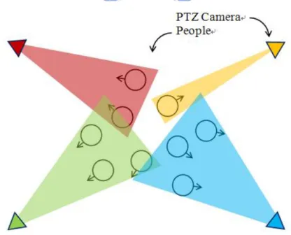
observe as many high-resolution faces as possible. In Figure 1-1, we illustrate the task of the proposed system. In this example, there are 9 people in total. The triangles denotes PTZ cameras, the circles indicate people’s locations, and the arrows represent the orientation of people’s face. The proposed system will automatically assign these four PTZ cameras to take care of different groups of people so that the multi-camera system can capture as many high-resolution facial images as possible at every moment.

We first formulate the problem according to some criteria and we define the evaluation function. We also try to optimize the evaluation function in an efficient way. For the sake of cost and convenience, we simulate the proposed system by using virtual videos generated from the ObjectVideo Virtual Video (OVVV) software tool.

In this thesis, we will first discuss some related works and mathematical techniques in Chapter 2. In Chapter 3, we will present the proposed coordination system which use multiple active cameras to get as many clear people’s face images as possible. Some experimental results are shown in Chapter 4. Finally, we give our conclusion in Chapter 5.

3

Chapter 2.

B

ACKGROUNDS

Although several multi-camera surveillance systems have already been proposed, we have not found any multi-camera system that offers similar functionalities as ours. Hence, we only mention a few articles that have discussed some issues similar to ours. In the proposed method, we use some mathematical techniques, such as clustering and optimization. Hence, we will also briefly introduce these mathematical techniques. In the end of this chapter, we will introduce the virtual video tool which we have made use of.

2.1. S

URVEILLANCE

S

YSTEMS WITH

PTZ

C

AMERAS

In general, in a surveillance system with PTZ cameras, there are several static cameras and no less than one PTZ camera. With the PTZ cameras, we are able to carry out more intelligent surveillance, such as active monitoring. For example, if we are interested in people’s faces, we may control the PTZ cameras to focus on someone’s face and identify who the person is.

Most of these systems mainly focus on the capture of clear human images. For example, in [1] and [2], Micheloni proposed a system that contains a few static cameras and PTZ cameras. The resolution of the PTZ camera is higher than that of static camera. When a person appears, they estimate the 3-D location of the target and automatically control the pan angle and tilt angle of the PTZ cameras to capture the target’s high-resolution images. In their approach, each PTZ camera focuses on the tracking of a single target. Their results are shown in Figure 2-1.

4

Figure 2-1 The results of Micheloni’s proposed system [2]

On the other hand, [3] uses the cooperation of multiple PTZ cameras to reduce the spatial limit and to locate the targets’ positions. This system is composed of two major parts: camera agents and a support module. Camera agents carry out image processing and camera control, while the support module coordinates all camera agents. The overview of this system is shown in Figure 2-2.

Figure 2-2 Overview of Kim’s system [3]

In [4], the proposed surveillance system also contains multiple static cameras and PTZ cameras. The static cameras are used to estimate the 3D positions of the detected targets. Face detection is also used to determine whether a human face exists. Once if

5

a face exists, then they control a PTZ camera to capture a close-up of that face.

Figure 2-3 Block diagram of Hampapur’s 3D tracker [4]

Figure 2-3 shows the 3D tracking process of the static cameras and Figure 2-4 shows how the system coordinates the static and PTZ cameras to accomplish face capturing. In Figure 2-5, we show the zoomed images captured by the PTZ camera.

In [5], the authors use pairs of static cameras to estimate the depth information. The face position of the target is estimated by combining the depth information with the face detection results. Similarly, once if a face is detected, a PTZ camera is controlled to capture a clearer facial picture of the target. Some experimental results are shown in Figure 2-6.

6

Figure 2-4 The process of face focus of Hampapur’s system [4]

Figure 2-5 A face zoom sequence [4]

In [6] and [7], the authors use pairs of static cameras to estimate the depth information. The face position of the target is estimated by combining the depth information with the face detection results. Similarly, once if a face is detected, a PTZ camera is controlled to capture a clearer facial picture of the target. Some examples are shown in Figure 2-7.

7 Figure 2-6 The experiment results of [5]

.

(a)

(b)

Figure 2-7 A virtual train station designed by Qureshi (a) over views (b) close-up

8

2.2. C

LUSTERING

A

LGORITHMS

Clustering can be thought as a kind of classification method. When there are several data which have some kinds of similar properties clustering methods can be used to explore the data and to group similar ones together under certain criteria. A clustering example is illustrated in Figure 2-8. In the literature, clustering has already been well developed and many different algorithms have been developed. We will discuss some commonly used algorithms in this section.

(a) (b) Figure 2-8 A clustering example (a) data points (b) clustering result

2.2.1. K-

MEANS

C

LUSTERING

K-means is a simple and fast clustering algorithm. It was originally proposed in [8]. The main idea of K-means clustering is to iteratively minimize the variance of each cluster. At the beginning, k centroids are initialized and they represent the centers of clusters. Then, each datum is classified to a cluster according to the distances between the data point and the centroids. The data point is assigned to the cluster which has the shortest distance between its centroid and this data point. Finally, the mean of each cluster is calculated and is used to update the new centroid. The process is repeated until the positions of the centroids converge. The followings are the detailed steps of the k-means algorithm:

1. In the data space, choose k points as the initial centroids of clusters. 2. Assign each data point to the cluster which has the shortest distance

between its centroid and that data point.

9

4. Repeat Step 2 and Step 3 until these centroids are almost fixed. Then we get the final clustering result.

The advantages of the k-means method are its simplicity and low computational cost. It is very easy to implement the K-means algorithm. However, this method still has several disadvantages. For example, it is very sensitive to the choice of the initial centroids. It only minimizes the intra-cluster variance, but not the global variance. In other words, this method does not guarantee global minimization but only a local minimization. The global minimization depends on the appropriate selection of the initial centroids. There is an example of k-means clustering shown in Figure 2-9.

(a) (b)

(c) (d) Figure 2-9 An example of the process of K-means clustering (a) centroids

initialization (b)-(d) iteration (centroids recalculation)

2.2.2. F

UZZY

C-M

EANS

C

LUSTERING

Fuzzy c-means clustering technique [9] is similar to k-means but it allows data to belong to more than one cluster. This is why it is called fuzzy. We illustrate the difference between k-means clustering and fuzzy c-means clustering in Figure 2-10. Here we consider 1-D data points and two clusters (red and green). For k-means

10

clustering, each data point only belongs to one cluster, as shown in Figure 2-10 (a). With fuzzy c-means clustering, however, each data point can belong to more than one cluster with different degrees of cluster membership, as shown in Figure 2-10 (b).

(a) (b) Figure 2-10 The comparison of (a) k-means clustering (b) fuzzy c-means cluster algorithm

The objective of fuzzy c-means clustering and k-means clustering are the same. That is, we find the clusters that minimize their variances. Similar to k-means, the fuzzy c-means clustering needs to define an initial condition and then iteratively update the cluster centers. However, the difference is that the fuzzy c-means clustering directly initializes the degrees of the data points in each cluster and update them in each iteration. The detailed fuzzy c-means algorithm is described as follows:

1. Initialize uij, the degree of xi in the cluster j, where xi is a data point.

2. Calculate each center cj by means of the formula 1

1 N m ij i i j N m ij i u x c u = = ⋅ =

∑

∑

.

3. Use this formula

1 2 1 1 m C i j ij k i k x c u x c − − = ⎡ ⎤ ⎛ − ⎞ ⎢ _{⎜ ⎟} ⎥ = ⎢ _{⎜ − ⎟} ⎥ ⎢ ⎝ ⎠ ⎥ ⎣ ⎦

∑

to update each uij.

4. Repeat Step 2 and Step 3 until _max

{

(k 1) ( )k

}

ij uij uij ε

+ _{− <}

where m is a real number greater than 1, k is the iteration number, and ε is a real number between 0 and 1.

Although fuzzy c-means clustering requires more computations than k-means clustering, it usually can find better solution. However, it still possesses some problems of k-means clustering. For example, it can only find a local minimum. The

Degree of cluster membership

P

Degree of cluster membership 1

11

clustering result is also sensitive to the initialization of the degrees.

2.2.3. H

IERARCHICAL

C

LUSTERING

Unlike k-means clustering and fuzzy c-means clustering, the hierarchical clustering algorithm [10] does not need to set the number of clusters. Compared with k-means (or fuzzy c-means) clustering, this method uses the concept of mergence, instead of the concept of partition. It considers each data point a cluster initially and then merges data points gradually to reach a proper set of clusters. Figure 2-11 illustrates the simple merging process. Here we take each creature as a data point and we gradually clustering these six creatures into clusters.

Figure 2-11 An example of merging process

The followings are the detailed steps of the hierarchical clustering algorithm: 1. Consider each data point a cluster. Define the distances between each

pair of clusters.

2. Find the pair of clusters which has the closest distance.

3. Merge the pair of clusters with the closest distance into a new cluster. The number of clusters reduces one.

4. Repeat Step 2 and Step 3 until the number of clusters reduces to a value we desire.

Generally, the hierarchical clustering method better suits the characteristics of data. It does not need assign the number of clusters and can always reach the same result. However, this method has a major problem: its high computational cost. Its complexity is at least O(n2). Besides, because of the mergence, this method cannot undo what have been done previously.

Cat Lion Dog Wolf Human Orangutan

12

2.3. O

PTIMIZATION

We usually encounter the optimization problem in our daily lives. For example, when we prepare a trip, we often ask how we can arrange our transportation to reduce the traveling time to the destination. This is a simple example of the optimization problem. Typically, an optimization problem can be formulated in mathematics. In general, we describe these problems by using an objective function with or without constraints. The objective function and the constraints are composed of several unknown parameters. Then, we try to find the selection of parameters that gets the minimum or maximum of the objective function. In other words, we want to find the values of parameters which make the value of the objective function minimal or maximal. Depending on the problems we want to solve, the objective function can be defined in different ways. The objective function may be linear or nonlinear and can be either continuous or discrete.

So far, many optimization algorithms have already been proposed, like gradient decent, linear programming, Lagrange multiplier, and Karush-Kuhn-Tucker (KKT) condition [11], etc. However, these derivative-based and linear constrained algorithms do not suit the problems that are nonlinear or cannot be differentiated. Hence, people devise some other algorithms for these kinds of optimization problems. Here, we briefly introduce two effective algorithms – Particle Swarm Optimization (PSO) and Differential Evolution (DE).

2.3.1. P

ARTICLE

S

WARM

O

PTIMIZATION

2.3.1.1.

C

LASSICAL

PSO

Kennedy and Eberhart devise the particle swarm optimization algorithm, which is inspired by a sociological model [12][13]. Each particle represents a trial solution of the problem that we want to solve. In this algorithm, as implied by the name “particle swarm”, a large number of particles are generated. The PSO algorithm uses these particles to carry out multi-agent parallel search. Each particle has its own memory. They can “remember” their previous best positions that make the objective function minimal or maximal. In addition, the particles communicate with each other to get the best global position that achieves the global extreme in the past. One

13

particle moves to its next position according to its previous best position and the global best position in the past. The particles repeat the same steps and they gradually converge to the final position.

In mathematics, the objective function can be expressed as

( )

(

1, , ,2 n

)

f x = f x x … x Eq. 2-1

where x is the variable vector in the n-dimensional space. Here we assume that the problem we want to solve is a minimization problem and we would like to find a x_*

that minimizes Eq. 2-1.

First, a group of particles are initialized randomly. That is, we create a certain number of particles and allocate their initial positions and velocities randomly. The velocity defines where the corresponding particle should move to next time. The position and velocity of the i-th particle at Time t are denoted as t

i

x and t i v , respectively. The number of particles is initialized by the user. For each particle, we calculate the value of the objective function at its current position. Every particle keeps track of its best previous position that gets the extreme value of the objective function. We denote the best previous position as P_i . In the meantime, we also record the globally best position, which is denoted as P . Finally, the next velocity and _g position of each particle can be calculated by Eq. 2-2 and Eq. 2-3, respectively.

(

)

(

)

1 1 1 2 2 t t t t i i i i g i v+ = ⋅ +ω v cϕ ⋅ P x− +cϕ ⋅ P −x Eq. 2-2 1 1 t t t i i i x+ = +x v+ Eq. 2-3

where ω is the inertia factor, c1 and c2 are scalars, and ϕ₁ and ϕ₂ are random

numbers generated from the uniform distribution over the interval [0, 1]. The aforementioned process is repeated until the stop criterion is reached. The followings are the pseudo code of the PSO algorithm.

P

SEUDO

C

ODE

Initialization: Initialize the positions ( x ) and velocities (_i0 v ) of N particles _i0

randomly. Also initializeP_i and P . _g

Begin

While the stop criterion is not reached For i = 1 to N

14

Evaluate the value of objective function for each particle:

( )

t i f x If f x

( )

_it < f P

( )

_i do t i i P =x End do If f P

( ) ( )

_i < f P_g do g i P = P End do End for For i = 1 to N

(

)

(

)

1 1 1 2 2 1 1 ω ϕ ϕ + + + = ⋅ + ⋅ − + ⋅ − = + t t t t i i i i g i t t t i i i v v c P x c P x x x v End for End while End

Output: the optimal position is x_*=P_g

The PSO algorithm is simple to implement without heavy computation load. In addition, it can find the global optimum and does not depend on the form of objective function (or fitness function). It is an effective optimization algorithm. We can utilize PSO to deal with complex, high-dimensional and nonlinear optimization problems.

2.3.1.2.

D

ISCRETE

B

INARY

PSO

The PSO algorithm mentioned above is originally operated in continuous domain. However, many optimization problems are actually in a discrete domain. Hence, Kennedy and Eberhart proposed the discrete binary version of PSO [14] for discrete optimization problems. The concept of discrete binary PSO algorithm is the same as the original PSO algorithm, except a few modifications over the original PSO algorithm. In the discrete binary space, the variables are only the integers 0 or 1. Hence we re-define the objective function (or fitness function) to Eq. 2-4:

15

( )

(

1, , ,2 n

)

f x = f x x … x Eq. 2-4

where x denotes an n-bit string, and xk represents the k-th bit which is 0 or 1 in the bit

string. Similarly, we want to find a x to minimize Eq. 2-4. The position of the i-th _*

particle and its d-th bit are denoted by xi and xid. The definition of velocity is different

from the original PSO. In continuous PSO, the velocity is defined for each particle. Here each dimension has its own velocity which is denoted by vid. That is, each bit has

its own velocity. Moreover, the velocity of the original PSO indicates where the corresponding particle moves to. However, when we discuss the velocity of binary PSO, we focus on each single bit and the meaning of velocities is changed. The meaning of velocity now represents the tendency of the corresponding bit to become 1. The larger the velocity is, the more likely the corresponding bit becomes 1. Besides, with the modification of the definition of velocity, the best previous position and the best previous global position are also treated in a bitwise manner. pid denotes the best

previous d-th bit of the i-th particles and pgd denotes the best previous global d-th bit.

Of course pid and pgd are either 0 or 1. With the above modifications, we rewrite the

velocity updating formula to be

(

)

(

)

1 1 2 t t t t id id id id gd id v+ _{= ⋅}ω v _{+ ⋅}ϕ p ₋x ₊ϕ _⋅ p ₋x Eq. 2-5 where t represents the time instant, ω is the inertia factor, and ϕ₁ and ϕ₂ are random numbers generated from the uniform distribution over the interval [0,1]. The authors used probability to describe the tendency of bit change so the velocities have to be converted to the interval [0, 1]. They introduce the sigmoid function and modified the position-updating formula to be defined as below:

( )

( )

(

1

)

1 1 0,1 1 0 t t id id t id if rand S v then x else x + + + < = = Eq. 2-6

where rand(0,1) is a random number selected from the uniform distribution over [0, 1], and S is a sigmoid function. Eq. 2-7 is the formula of the sigmoid function.

( )

1 1 v S v e− = + Eq. 2-7

The logistic curve of the sigmoid function is shown in Figure 2-12. This function transfers the value of vid into the interval [0, 1].

16 Figure 2-12 Sigmoid function

Basically, the binary PSO is very similar to the original PSO. Only the definition of velocity and the position-updating function are modified. The followings are the pseudo codes of the DBPSO algorithm.

P

SEUDO

C

ODE

Initialization: Initialize the positions (x ) and velocities (_i0 v_id0 ) of N particles

randomly. Also initialize pi and pg

Begin

While the stop criterion is not reached For i = 1 to N

Evaluate the value of objective function of each particle:

( )

t i f x If f

( )

xt_i < f

( )

p do _i t i = i p x End do If f

( )

p_i < f

( )

p_g do g = i p p End do End for For i = 1 to N For d = 1 to n

17

(

)

(

)

( )

( )

(

)

1 1 2 1 1 1 0,1 1 0 ω ϕ ϕ + + + + = ⋅ + ⋅ − + ⋅ − < = = t t t t id id id id gd id t t id id t id v v p x p x if rand S v then x else x End for End for End while End

Output: the optimal bit string is x_* =p _g

The binary PSO inherits the main concept from the original PSO. The particle swarm still has “memory” in the binary PSO and the particles move toward the region that so far provides the best solution. The DBPSO is also effective for solving the discrete binary optimization problems.

2.3.2. D

IFFERENTIAL

E

VOLUTION

Differential evolution is a global optimization algorithm proposed by Storn and Price [15]. Like PSO, it is one kind of parallel searching techniques. It generates several numbers of trial parameter vectors at the same time and tries to find the optimum. DE inherits the ideas from genetic algorithm but it alters the classical crossover and mutation operqations. The authors present a differential operator to generating new “offspring” for the searching of the optimum. The block diagram of the DE algorithm is shown in Figure 2-13.

Figure 2-13 The block diagram of differential evolution algorithm [16]

In the initialization stage, a population is initialized. In other words, a number of D-dimensional parameter vectors are initialized. The i-th parameter vector in the g-th generation is denoted as g

i

x , and the population size is denoted as N. After the initialization, DE creates several candidates that may become parts of the population of the next generation. These candidates are generated by means of “mutation” and “crossover”. In the mutation stage, we use Eq. 2-8 to generate a “mutant” parameter vector for each target vector, g

i x :

18

(

)

1 2 3 1 g g g g i r r r v + ₌x _{+ ⋅}C x ₋x Eq. 2-8 where C is a constant in [0, 2] and r1, r2, r3 are the random integers from 1 to N. In

Figure 2-14, we show an example of mutation.

Figure 2-14 A mutation example of a two dimensional minimization problem [15]

Next, the mutant parameter vectors are carried out crossover to increase the variance. A trial parameter vector, g

i

u , is created for each target vector by means of crossover. It is generated based on the following equation:

( )

( )

1 , 1 , , , 0,1 1, , + + _{= ⎨}⎧⎪ ≤ = ⎪⎩ g i j int g i j g i j v if rand CR or j rand D u x otherwise Eq. 2-9

where j is an integer from 1 to D that represents the value of the j-th dimension; rand(0, 1) is a random real number generated from the uniform distribution over [0, 1]; randint(1, D) is a random integer number chosen from {1, 2,…, D}; and CR represents

the pre-defined crossover constant within the range [0, 1]. In Figure 2-15, we illustrate the crossover process.

19

Figure 2-15 An example of crossover [15]

Finally, the selection process is performed to decide the next-generation population. Here we assume that we want to find the minimum of the objective function. A decision is made by comparing the target vector with the corresponding trial vector. If the trail vector produces the smaller value of objective function (or fitness function) than the target vector, the target vector will be replaced by the trail vector as the next-generation population. On the contrary, the target vector is retained. Eq. 2-10 formulates the selection process:

( ) ( )

1 1 1 , , + + + _{= ⎨}⎧⎪ < ⎪⎩ g g g i i i g i _g i u f u f x x x otherwise Eq. 2-10

where f is the objective function (or fitness function) to be minimized.

Differential evolution imitates the biological behavior and tries to find the global optimum of the multi-dimensional objective function in the continuous space. It is also easy to be implemented and is an effective global optimization algorithm.

20

2.4. V

IRTUAL

V

IDEO

T

OOL

In general, we have to set up real cameras to verify the proposed surveillance system. From time to time, we need to change the experimental environments and the adjustment may cost a lot money and time. Hence, using virtual reality for experiments is another choice to release the dilemma. In the literature, there have been some examples, like [17] and [18], that use virtual reality tools to help the development of their surveillance systems.

In [19], Taylor et al. developed a virtual video tool for surveillance simulation and evaluation. They call it ObjectVideo Virtual Video (OVVV), which is a modification based on the game engine of Half-Life 2 by Valve Software. It can simulate static or active cameras and render video streams. In addition, it can also extract the ground truth from each camera automatically to help performance evaluation.

Figure 2-16 shows the block diagrams of the OVVV system. The camera server manages the virtual cameras which are defined by several camera parameters, including frame rate, orientation, location, and field of view (FOV). This system can render videos for each virtual camera. The PTZ server controls the PTZ parameters of each virtual camera. Because of the utilization of TCP/IP (Transmission Control Protocol/Internet Protocol) protocol, we can access the camera and PTZ servers via internet. We can get the videos generated by virtual cameras and adjust the PTZ parameters of each camera remotely through the video client and PTZ client. Moreover, we do not necessarily operate them on only one computer. In other words, we can manipulate them even on the computer where the OVVV system is not installed.

21

OVVV system is not just a simple virtual video generator. In order to simulate real cameras, several kinds of noise and camera distortion can be added optionally, including additive pixel noise, video ghost, radial distortion, blur, defocus, and jitter. Users can also change the level of noise or distortion arbitrarily. Based on these functionalities, we’ll be able to discuss the relationship between noise interference and the performance of the surveillance system. An example of noise addition is shown in Figure 2-17. Besides noise and distortion, the OVVV system can also simulate omni-cameras, such as panoramic and parabolic catadioptric omni-directional cameras. These two kinds of cameras views are shown in Figure 2-18. These functions can increase the usability for many kinds of surveillance experiments.

Figure 2-17 The synthetic frames with (right) and without (left) noises [19]

Figure 2-18 The synthetic frames of omnicams: panoramic (left) parabolic

catadioptric (right) omni-directional cameras [19]

OVVV system does not only aim at simulation but evaluation. It can generate the ground truth to support the evaluation of surveillance systems. It includes both camera and target ground truth. The camera ground truth consists of camera center, camera orientation, horizontal FOV, and frame dimensions. The target ground truth consists of 3D world location of target center, target center on image, foreground label map, bounding box of an entire target, and bounding box of a visible target. Figure 2-19 shows an example of the ground truth. In the left figure of Figure 2-19, the dashed line represents the bounding box of an entire target and the solid one represents the

22

bounding box of visible target. The different bounding boxes help us to evaluate the performance of the system under the occlusion situation.

Figure 2-19 A ground truth examples: bounding box (left) and label map (right) [19]

Because the scenarios and scripts are simulated virtually, we can repeat the experiments with the same experimental environment to improve our surveillance system. In addition, we can acquire those sequences that are hard to make. We can also place cameras at any place and can control these cameras easily. Although eventually we still have to test our surveillance in the real world, the use of the OVVV tools can shorten the period of system development and increase the feasibility of the developed system. With the help of the OVVV system, we can greatly reduce the cost of development.

23

Chapter 3.

C

AMERA

C

OORDINATION

Figure 3-1 shows the flow chart of our proposed coordination system. In this thesis, focus on the coordination of multiple cameras. Here, we assume all pre-processes, like camera calibration, object detection, face detection, and object tracking, have already been done. Hence, the 3D locations of the targets and the orientations of the target faces are available beforehand. Here we utilize the ground truth of OVVV to accomplish these tasks. In this chapter, we’ll discuss how to formulate the coordination problem and how to apply a suitable optimization tool to achieve the goal.

Figure 3-1 Flow chart of our proposed camera coordination system

3.1. P

ROBLEM

F

ORMULATION

At the start, we define the problem that we want to solve. Unlike the articles we introduce in Section 2.1, we aim to capture as many frontal high-resolution facial images as possible during the presence of the monitored targets. In the proposed

Optimization

Camera

Adjustment

Input Video

OVVV

Output Video

24

algorithm, PTZ cameras are allowed to cover more than one target at each time, as long as the captured facial images are sufficiently clear. Moreover, we allow the tracking of a target can be handed over from one PTZ camera to another PTZ camera so that the face of that target can be better observed over time. In the proposed algorithm, we design our camera coordination system based on two major criteria: frontal shoot and high-resolution shoot.

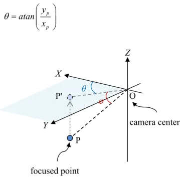
To formulate these two criteria, we define the shoot angle θij, and the face width

Wij. In θij and Wij, the subscript i denotes the i-th PTZ camera, while the subscript j

denotes the j-th target. As shown in Figure 3-2, the shoot angle θij represents the angle

between the blue arrow cam_ij and the green arrow face . _j cam_ij indicates the line connecting the i-th PTZ camera and the j-th target, while face indicates the facing _j orientation of the j-th target. As the j-th target is looking toward the i-th camera, we have a smaller shoot angle. On the other hand, as shown in Figure 3-3, the shot face width Wij represents the width of the j-th target’s face in the image captured by the i-th

camera. A larger value of Wij indicates a better observation of the j-th target in the the

i-th camera image.

Figure 3-2 The illustration of θij

Figure 3-3 The illustration of Wij

Wij

j-th Target The image of camera i

j face ij cam Camera i Person j ij θ

25

To simplify the computation of θij and Wij, all 3-D vectors are projected onto the

ground plan to form 2-D vectors instead of calculating 3-D vectors directly. In other words, we only consider the 2D vectors here in order to simplify the computation. In the simplified forms, the shoot angle and the face width are defined as follows.

( ) θ = ij⋅ j ij ij j cam face acos

cam face Eq. 3-1

3

ij xi

ij

Face width in D space W f D = _{Eq. 3-2} 2 2 xi i Image width f FOV tan = ⎛ ⎞ ⋅ _{⎜ ⎟} ⎝ ⎠ Eq. 3-3

In the definition of Wij, fxi denotes the focal length of the i-th PTZ camera in the

horizontal direction, Dij is the distance between the i-th camera and the j-th target, and

FOVi is the field of view of the i-th PTZ camera. Eq. 3-2 and Eq. 3-3 originate in the

pinhole camera model. Originally Eq. 3-2 is used only when the face is on the center of image. However, we do not need a very precise face width in the image. Hence, we simply define the face width in an approximated way to simplify the computation.

The shoot angle and the face width are two different physical quantities. In addition, the desired tendencies of the two quantities are different. Basically, we prefer to capture a facial image with a smaller shoot angle but a larger face width. Therefore, we apply two mapping functions Nθ( ) and Nw( ) over θij and Wij to convert

them into two normalized measures. The two different quantities can be unified after normalizing. Here we define the values to become lager after normalizing when the performance we desire is became well. In other words, we set higher “scores” for better capture situations. For example, we hope that θij is as small as possible so that

we can see more frontal face. Therefore, the value of Nθ(x) becomes lager as the x

becomes smaller. These two mapping functions are defined as follows and are illustrated in Figure 3-4 and Figure 3-5.

( )

(

1 2

)

, 0 0 , otherwise r k r k x x th N x th θ θ θ θ θ + ⎧₋ ⋅ _{+ ≤ <} ⎪ = ⎨ ⎪ ⎩ Eq. 3-4

26

( )

(

)

(

)

0 , 1 , 2 1 , 2 min W W W min W min max

max min max min W max x th r k r k r k th N x x th x th th th th th r k x th ⎧ ⎪ _< ⎪ − ⎪ ⋅ ⋅ ⋅ =_⎨ − + ≤ < − − ⎪ ⎪ ₊ ⎪ ≥ ⎩ Eq. 3-5

In Eq. 3-4 and Eq. 3-5, k is a positive constant that controls the dynamic range of Nθ( ) and Nw( ). rθ and rW are real numbers within the range [0, 1] and they control

the slopes of Nθ( ) and Nw( ). thθ, thmin, and thmax are pre-defined thresholds. thθ

represents the worst situation that can be allowed for capturing the frontal face. thmin

represents the minimum face width for clear observation. On the other hand, when the face width is wider than thmax, we think the facial image has achieved the level of

perfect observation. These thresholds can be varied by the users for different applications.

Figure 3-4 Normalized function of the bias angle

0 x

( )

W N x

(

1

)

2 W r k − max th

(

1

)

2 W r k + min th 0

( )

N x_θ x

(

1

)

2 r k θ −

(

1

)

2 r k θ + th_θ

27

Figure 3-5 Normalized function of the face width

The physical meaning of thθ is the worst situation for capturing the frontal face.

In other words, we hardly clearly see (or identify) someone’s face when the angle between face vector and camera vector exceeds thθ. Similarly, thmin and thmax represent

the worst and best case of face width in the image respectively. When the face width is smaller then thmin, we also hardly see the clear face because of the low resolution.

Conversely, when the face width reaches or exceeds the threshold, thmax, we can

clearly to identify this face. The function of rθ and rW are to adjust the slopes of the

linear part of the normalized functions and the maximal and minimal values of the normalized functions. It will affect the weightings of the orientation and clearness. For example, if rW becomes smaller, the largest and smallest values of the normalized

function will be closer and the difference between them is smaller. That means the discrimination of the face resolution is decreased. Under the extreme condition, if we let the rW be zero (and it will make the slope zero), any face width will get the same

normalized value. That makes no difference no matter what the face width is after the normalization.

The goal is that our system finds a camera coordination way to make each θij as

small as possible while make each Wij as large as possible. With the definitions of Nθ and NW, we then define Eval( ) (Eq. 3-6) for the face capture of the j-th target by the

i-th camera. It is defined to evaluate the different coordination. The large the value of Eval( ) is, the better the performance of coordination is.

( )

( ) ( )

1 1 m n ij ij W ij i j Eval AP ap N_θ θ N W = = =

∑∑

_{Eq. 3-6}

In Eq. 3-6, m and n are the number of cameras and targets respectively. AP denotes a set of camera assignments and is defined as Eq. 3-7:

{ }

_ij , 1, 2, , , 1, 2, ,

AP= ap i= … m j= … n Eq. 3-7

apij represents the binary assignment parameters. apij is equal to 1 if the i-th camera is

assigned to monitor the j-th target, and apij is equal to 0 otherwise. Hence, for a

camera assignment AP, Eval(AP) represents the overall observation levels of the n targets by all m cameras. When more targets can be better observed by their corresponding cameras, with smaller shoot angles and larger face widths, we have a larger Eval(AP). Hence, the goal of the proposed camera coordination system is simply to find the optimal camera assignment that reaches the largest Eval(AP). Moreover, as these n targets keep moving within the monitored scene, we need to

28

adaptively adjust the assignment of cameras to achieve the most preferable observation.

Besides, to simplify the problem, we also add one extra constraint over Eq. 3-6. The constraint is stated in Eq. 3-8:

1 1, 1, 2, , m ik i ap k n = = =

∑

… Eq. 3-8

This constraint implies that we only take into account the camera view that is assigned to the target even though that target may also appear in some other views.

Because there are two criteria, one target has two observation level, the level of orientation (shoot angle) and the level of clearness (face width). They are the values of the two normalized functions, Nθ and NW, respectively. The zero values of the

normalized functions mean that the situation of orientation or clearness is too bad to identify the target’s face. Here, we multiply these two scores together to form the final score. This is because we consider these two scores to be dependent. We consider that if one of the scores for a target is low, we will not be able to clearly see that target even though the other score is high. Hence, as one score is high but the other one is low, the final score is still low. In addition, when the performance of orientation or clearness is lower than a threshold, according to Eq. 3-4 or Eq. 3-5, the value of Eq. 3-6 (total score) is set to zero.

We add all the targets’ overall observation levels together to evaluate the performance of camera coordination for all targets. Obviously, according to the mapping functions we define, the value of the evaluation function (Eq. 3-6) will become larger if the performance of coordination gets better. That is to say, more frontal and higher resolution faces. Thus, the goal is that we want to find a set of camera assignment (assigned parameters), AP, which makes the evaluation function maximal. In other words, we want to find an optimal AP here.

3.2. S

IGNIFICANCE WEIGHT

In theory, we can always find an optimal AP for the evaluation function at any time instant. However, people’s behavior is highly diverse. It is very likely that even with the optimal camera assignment we still cannot clearly capture all people’s faces at some time instants. In addition, the evaluation function takes all people into

29

account and the evaluation function is actually a tradeoff among all cameras. It may happen that some people’s observation levels are sacrificed to gain other people’s observation levels. Hence, the proposed system cannot guarantee that all people’s faces are always clearly observed.

Because the evaluation function takes all people into account, sometimes the tradeoff situation happens when we carry out the optimization. It means that maybe some people’s observation level is sacrificed to increase some other people’s observation level. The increased value of evaluation function may be larger than the sacrificed value so the system will prefer this kind of coordination during the optimization process. Figure 3-6 shows an example of the optimization tradeoff. In Figure 3-6, two different cases are illustrated. Compared with Figure 3-6(a), Camera 2 in Figure 3-6(b) cannot capture Person 3’s frontal face and we lose some scores on it. However, the FOV of Camera 1 becomes small because Camera 1 only needs to take charge of Person 1 and Person 2. As the FOV becomes smaller, the scores of Person 1 and Person 2 increase. The total increased amount is larger than the decreased amount and the total scores become higher.

The cases that the system cannot always cover all people’s faces are unavoidable. However, we still hope to clearly see the unclear faces in the next moment. We hope we’ll be able to clearly see all people’s face during some periods of time and try to capture as many frontal high-resolution facial images as possible.

To deal with this problem, we assign each target a significance weight to represent the priority of that target. In other word, it represents the importance of the target. This weight will increase if the target hasn’t been clearly observed in the past few moments. On the contrary, if that target has already been clearly observed for a while, we decrease its significance weight. Here, target’s “clearness” is defined by his/her observation level. The zero observation level means that the corresponding target cannot be observed at all.

30

(a) (b)

Figure 3-6 (a) lower (b) higher overall observation level

3.2.1. W

EIGHTING

U

PDATE

The usage of significance weight is to help the clear capture of targets’ faces. The values of weights are closely related to the situation that targets cannot be clearly captured. The trend of significance weight roughly follows the states of the clearness. Here, we design the adjustment of significance weight to include three major states: rise, hold, and decline.

3.2.1.1.

R

ISE

S

TATE

The weight increases continuously in the rise state. When the face of a target cannot be clearly captured, we linearly increase its significance weight. When the weight is raised, the system will pay more attention to that target and it’s more likely that the target can be better observed. The value of weight is 0 initially. When a target’s face is unclear, his or her weight starts to increase. If the unclear situation is continuous, the value will also increase continuously. It will stop increasing when the unclear situation is improved.

3.2.1.2.

H

OLD

S

TATE

Once if the system has adjusted its camera coordination to take clear facial Camera 1 Camera 2 People 1 2 3 4 5 Camera 1 Camera 2 People 1 2 3 4 5

31

picture of that target, the significance weight will be held at a high value for a while. At this time, we stop to increase the value of the significance weight because we have already clearly seen the target’s face. Although we stop to increase the weight, we do not decrease the value of weight immediately. This is because we hope we can clearly see the person’s face for a while, but not just a short glimpse. Hence, the significance weight is held in the holding state for a pre-defined period to ensure the target’s face can be clearly observed for a long enough period.

3.2.1.3.

D

ECLINE

S

TATE

After keeping a period of “hold”, the significance weight of the target is decreased gradually as long as the target’s face can be clearly captured. This is because we have paid attention to the target for a long enough period in the holding state and the target is no longer as important as before. Similar to the rise state, we reduce the value linearly. The value will be continuously reduced to zero as long as the target’s face can be clearly captured continuously.

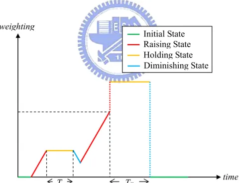
These three states are alternately taken place until the weight comes back to the initial state, that is, the zero value. Once a target’s face becomes unclear, his/her weight is in the “rise” state again. As the target’s face can be clearly observed, the state switches to “hold” for a while. If the face is continuously clear after a period of time, the state will switch to the “decline” state. However, if the face becomes unclear suddenly during the “hold” or “decline” state, it will switch back to the “rise” state to enforce a higher priority in capturing the clear image of that face.

Figure 3-7 Variation of the significance weight over time

An example of the switching of these three states is illustrated in Figure 3-7. At the beginning, the target’s face is not clear within the “rise” state. T represents the

time weight Initial State Rise State Hold State Decline State T T

32

holding time. As illustrated in Figure 3-7, whenever the unclear condition happens, the “rise” state takes place again. On the other hand, as the target can be clearly observed for a while, the weight drops to zero in the “decline” state.

3.2.2. U

PPER

B

OUND OF

U

NCLEAR

P

ERIOD

Although the significance weight can help us in alleviating unclear observation, it still takes a while for an unclear observed target to get clearly observed. In some situations, the lag can be too long for practical usage. Hence, we put an upper bound over the unclear period. If the time period that a target hasn’t been clear observed exceeds a pre-defined threshold, its significance weight is dramatically raised to a very large value. This pushes the camera coordination system to take quick response to take good care of that target.

As we dramatically raise the weight to a very large value, the people who are unclear before will have a very high priority to be clearly captured. Similar to the hold state mentioned in Section 3.2.1.2, this large value is also held for a long enough period. However, this period can be different than the aforementioned “hold” period. Moreover, the value of the weight is reset to zero this time when the high-value hold process ends, as illustrated in Figure 3-8.

On the other hand, we also take the value of significance weight into account. When the value of the weight increases to a certain level but the corresponding target is still not captured well, we also adjust the target’s significance weight to a very high value, as illustrated in Figure 3-9.

33

Figure 3-8 Illustration of the weighting variation for the case of time limitation

Figure 3-9 Illustration of the weighting variation for the case of weighting limitation

 

time weighting Initial State Raising State Holding State Diminishing State T Tlh time weighting Initial State Raising State Holding State Diminishing State T Tth Tlh

34

3.2.3. C

OMBINING

W

EIGHT WITH

E

VALUATION

Because we want to take significance weight into account when we adjust the camera coordination, we incorporate significance weight into the evaluation function. Our object is that a target with higher weight will have a higher priority to be clearly captured. To realize the concept of importance weight, we add penalty term into the definition of Eval( ). If a target is assigned to a camera which cannot clearly capture his/her face by an AP, the evaluated value of the AP will be added a penalty term. This causes a value to be deducted from the original evaluated value. Hence, we redefine the evaluation function as below:

( )

(

( ) ( )

)

1 1 m n ij ij W ij ij i j Eval AP ap Nθ θ N W pv = = =

∑∑

− Eq. 3-9

where the penalty term pvij is defined as

ij ij j p

pv =cf sw c⋅ ⋅ Eq. 3-10

In Eq. 3-10, swj stands for the significance weight of the j-th target, cfij represents the

clear factor of the j-th target with respect to the i-th camera, and cp is a controlling

parameter. The clear factor cfij is equal to 0 if the j-th target can be clearly observed

by the i-th camera. Otherwise, cfij is equal to 1. Apparently, the penalty value is

determined by the significance weight. The higher the weight is, the larger the penalty value is. With the inclusion of the penalty term, the camera coordination system can automatically pay more attention to these targets with larger significance weights.

3.3. M

ODIFIED

D

ISCRETE

B

INARY

PSO

In Eq. 3-9, we redefine our problem and want to find an AP to maximize the evaluation function. In mathematics, this is simply an optimization problem. Unfortunately, Eq. 3-9 has a nonlinear and non-differentiable form. To find the optimal AP, these classical optimization algorithms, like the gradient descent algorithm, cannot be used. Instead, we adopt the particle swarm optimization algorithm [12] mentioned in Section 2.3.1 to tackle this problem. Due to the binary nature of the assignment parameters, we actually adopt the discrete binary particle swarm optimization proposed in [14]. Moreover, since we have added one constraint in the evaluation function, we further make some modifications over the discrete

35

binary particle swarm optimization algorithm to tackle the problem.

According to the discrete binary PSO algorithm, the evaluation function Eq. 3-9 is equal to the objective function in Eq. 2-4. We want to find an AP that maximizes the evaluation function. AP is equivalent to the x in Eq. 2-4. Here, we can consider it as a bit string composed of a set of apij. An AP can be thought as a particle position

too. In the first step of DBPSO, we will generate a number of AP’s first.

3.3.1. P

ARTICLE

G

ENERATION

In the modified DBPSO, each particle represents a possible AP. In the original form of PSO, particles are randomly generated in the initial stage. The use of random particles increases the probability of finding the global optimum. However, this also causes a large number of iterations. To speed up the computations, we develop two simple but effective schemes to generate particles. At the first scheme, we utilize clustering to generate a reasonable initial guess about AP and use it to produce particles. In addition to the initial clustering over the monitored targets, we also utilize the temporal information in the second scheme to speed up the optimization process in subsequent frames.

3.3.1.1.

F

EATURE

S

PACE

In our approach, we consider that the people with similar characteristics should be assigned to the same camera. The characteristics we think are people’s positions and orientations. For the sake of efficiency, people who are close to each other and have similar face orientations are more likely to be assigned to the same camera. Hence, we use the clustering technique first for the design of camera coordination.

We first create a feature space and convert people’s characteristics into this space. In other words, the characteristics of each person correspond to a data point in the feature space. Here, we define the feature space based on people’s positions and orientations. We then perform clustering over the data points. For people’s positions, we consider the 2D coordinates (X,Y). For people’s orientations, we use the inner product of the camera vector and the face vector. The camera vector and face vector are illustrated in Figure 3-2. Here, we do not directly use the inner product of these two vectors. Instead, we check the cosine of the included angle between these two vectors.

36

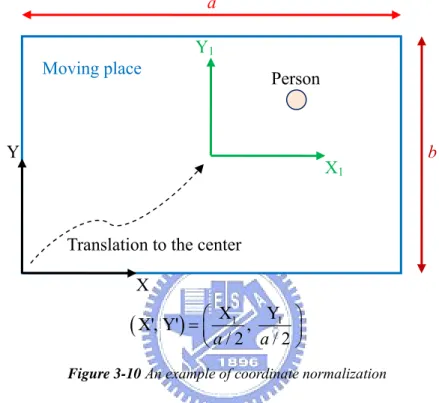
However, position and orientation are very different physical quantities. Hence, we further normalize these two quantities. Since the value of the cosine of the included angle is within the range [-1, 1], we normalize the positions to be within the same range. That is, the origin of the (X,Y) coordinates is translated to the center of the space. Then, the new coordinates of X and Y are divided by the half width of the space to get the normalized coordinates (X’ ,Y’), as illustrated in Figure 3-10.

Figure 3-10 An example of coordinate normalization

In Figure 3-10, we use a to normalize the position because it is longer than b. With this normalization, the values of X’ and Y’ are in the range [-1, 1].

Assume m is the number of cameras. We define the dimension of the feature space to be m+2. For example, as we install four PTZ cameras, the feature space has 6 dimensions and each target corresponds to a 6-D data point as expressed in Eq. 3-11:

(

λX', Y', , , , λ IP IP IP IP1 2 3 4

)

Eq. 3-11

where λ is a scalar to balance between positions and orientations. In Eq. 3-11, X’ and Y’ represent the normalized coordinates of the target on the ground plane. Both X’ and Y’ have the range [-1, 1]. IPi represents the normalized inner product between

j

face and cam . IP_ij i has the range [-1, 1]. Moreover, because the orientation

characteristic has m dimensions but the position one only has two, we use λ to balance it. In this case, we choose λ = 2.

X Y

X1

Y1

Moving place

Translation to the center

Person a b

(

_{X', Y'}

)

X1 _, Y1 / 2 / 2 a a ⎛ ⎞ = ⎜_⎝ ⎟_⎠