利用雙波長飛秒脈衝激發光子晶體光纖產生紫外超連續光譜之數值分析

全文

(1)國立交通大學光電工程研究所碩士論文利用雙波長飛秒脈衝激發光子晶體光纖產生紫外超連續光譜之數值分析. Numerical Simulation of UV Enhancement of Supercontinuum Generation by Injecting Dual Wavelength femtosecond Pulses into Photonic Crystal Fibers. 研究生：陳億文指導教授：謝文峰. 教授. 中華民國九十七年六月.

(2) 利用雙波長飛秒脈衝激發光子晶體光纖產生紫外超連續光譜之數值分析 Numerical Simulation of UV Enhancement of Supercontinuum Generation by Injecting Dual Wavelength femtosecond Pulses into Photonic Crystal Fibers 研究生：陳億文指導教授：謝文峰. Student：Yi-Wen Chen 教授. Advisor：Wen-Feng Hsieh 國立交通大學光電工程研究所碩士論文. A Thesis Submitted to Institute of Electro-optical Engineering College of Electrical Engineering and Computer Science National Chiao Tung University in Partial Fulfillment of the Requirements for the Degree of Master in Electro-optical Engineering June 2007 Hsinchu, Taiwan, Republic of China. 中華民國九十七年六月.

(3) 利用雙波長飛秒脈衝激發光子晶體光纖產生紫外超連續光譜之數值分析. 研究生：陳億文. 指導教授：謝文峰教授. 國立交通大學光電工程研究所. 摘要為了使光子晶體光纖產生的光譜有效的延伸到紫外光的波段，在這篇論文中，我們利用飛秒鈦藍寶石脈衝雷射產生的基頻以及倍頻光同時打入光子晶體光纖中，做了數值模擬以及實驗觀察，研究這兩道光脈衝在時空上重疊時所產生的交叉相位調變作用，使得產生的光頻譜有效地往短波長延伸。在數值模擬中，我們利用分離步驟法去求解藕合非線性薛丁格方程，發現利用 790 nm 以及 395 nm 的光脈衝同時導入光子晶體光纖 NL-PM 760 中，在短波長的部分產生的光譜最連續且平坦，此效應會隨著兩道光脈衝峰值功率的增加變得更加明顯。但是在實驗觀察中，紫外光的光頻譜展開並沒有理論預測的明顯，推論這是因為短波長的光在光子晶體光纖中有嚴重的損耗，或是因為倍頻光影響了光的耦合條件，使得輸出的超連續光譜不如理論預測。. i.

(4) Numerical Simulation of UV Enhancement of Supercontinuum Generation by Injecting Dual Wavelength femtosecond Pulses into Photonic Crystal Fibers. Student： Yi-Wen Chen. Advisor： Prof. Wen-Feng Hsieh. Institute of Electro-optical Engineering National Chaio Tung University. Abstract In order to make the further extension of the generated spectrum to the near UV part, we do the simulation and the experimental investigation on the supercontinuum generation using the fundamental and its second harmonic femtosecond pulses from a Ti:sapphire laser into the photonic crystal fiber simultaneously.. When these two color pulses are spatially and. temporally overlap in the photonic crystal fiber, the cross phase modulation will extend the spectrum toward short wavelength.. In the simulation, we use the Split-Step Fourier Method. to solve the coupled nonlinear Schrödinger equation.. The most continuum and flattened. spectrum on the UV part can be generated by using the dual wavelengths of 790 nm and 395 nm.. The spectra become more and more continuous and flattened as the input peak power of. these two pulse increase.. Nevertheless, in the experiment, the spectrum on the UV part does ii.

(5) not become broadened as expected in our simulation results.. It might be due to the seriously. loss on the UV part or the change of coupling efficiency resulted from thermal expansion by the launch of the second harmonic pulse to change the core size and the value of numerical aperture.. iii.

(6) 致謝還記得剛進實驗室是我大三的時候吧，轉眼就要碩二畢業，不知不覺間已經在老闆實驗室裡待了三年半，在這段歲月中，充滿著歡笑與感動，很慶幸這段時間我過得很充實，學到了很多很多，不管是學問上，或是做人處事、人際關係等等。而這一切一切，也要感謝很多人對我的指教。首先，我要感謝老闆在這些年來的照顧，帶著我們研讀論文，培養口頭報告的技巧，教導我們研究態度與方法，以及在為人處世等各方面都花費心思地細心指導，尤其在義大利報告的那段時間，如果不是老師和師母如家人一般的照顧，還帶著我們四處遊玩，我想義大利之旅可能是不斷的問路、迷路以及破產吧@@，此外，我還要特別感謝家弘學長在研究生涯中給予我的幫助，與你不時的討論中，總給予我正確的方向，使我獲益匪淺。當然，在這兩年的生活中，並不只有實驗與研究而已，還和實驗室裡的夥伴們培養了深厚的情誼。碩二的朋友們，陳博，這兩年應該跟你最熟了吧，從你被小豪拐去 CANON 的陣營之後，就常常有機會一起討論相片，學術上很多不會的問題到你手上，也總能迎刃而解，陳博啊陳博，你真不愧是陳博啊!!!；小詹，感謝你總是願意當我說冷笑話時的罐頭笑聲；小新，你真是實驗室裡的開心果，我想這實驗室如果沒有你的話，也許就沒有這麼熱鬧囉；老徐，成為百大富豪的時候要記得我是你同學嘿；五佰，跟你同窗已經五年了，可是真正跟你比較有互動卻是在這最後一年，只能說，你怎麼把我的八卦都挖出來了>///<；香腸，真後悔沒有跟你學兩招，不然以後失業或許還能去當股市名嘴 XD。另外，還有實驗室雷射組的大師兄、智章和博濟學長以及光晶組的智賢學長，感謝你們在這段期間給予我很多的指導和意見。材料組的小豪學長，謝謝你教我很多攝影上的知識與技巧，還有你對改寫程式的認真與執著真是讓我大開眼界對你刮目相看，此外還有松哥、黃董、小郭、維仁、信民、國峰學長、水晶晶學姐，雖然這段時間與你們相處的時間並不多，不過感覺你們都是很好的人，沒有與你們有更多的互動感覺還蠻遺憾的。最後，實驗室的肥肥、棕儂、大隻佬、建輝學弟、智雅、小布丁學妹們當然也不能忘記，你/妳們的幫忙及搞笑我銘感在心，你們送的花和卡片真的讓人就甘心。另外，還要感謝我的家人以及女朋友在背後的默默支持更是我前進的動力，給予我體諒、包容以及全力的支持，最後感謝國科會 NSC96-2628-M-009-001-MY3 計劃的支持，讓我的研究得以順利完成。 2008.07.14 陳 IC 於交大. IV.

(7) Contents Abstract (in Chinese)…………………………………………………………………………...I Abstract (in English)…………………………………………………………………………..II Acknowledgements………………………………………………………………………….IV Contents………………………………………………………………………………………V List of Figures……………………………………………………………………………...VIII. Chapter 1. Introduction…………………………………………………………1. 1.1. Photonic Crystal Fibers…………………………………………………………………..1. 1.2. Supercontinuum Generation……………………………………………………..............3. 1.3 Third Order Nonlinear Optical Effects…………….…………………............................4 1.3.1 Self-Phase Modulation……………………………………………………...............5 1.3.2. Cross-Phase Modulation……………………………………………………………6. 1.3.3. Degenerate Four-Wave Mixing……………………………………………..............7. 1.3.4. Modulation Instability……………………………………………………...............8. 1.3.5. Stimulated Raman Scattering………………………………………………………9. 1.3.6. Self-Steepening……………………………………………………………………10. 1.3.7. Higher-Order Dispersion…………………………………………………………..10. 1.4. Motivation……………………………………………………………………...............11. 1.5. Organization of this Thesis……………………………………………………..............12. Chapter 2. Simulation of Nonlinear Schrödinger Equation………………….13. 2.1. Coupled Nonlinear Schrödinger Equation……………………………………..............13. 2.2. Fourier Transform…………………………………………………………....................17 V.

(8) 2.2.1. Discrete Fourier Transform……………………………………………………….18. 2.2.2. Fast Fourier Transform……………………………………………………………20. 2.2.3 Convolution Theory………………………………………………………………22 2.3. Split-Step Fourier Method…………………………………………………………….23. 2.4. Verification of the Simulations………………………………………………………...29. Chapter 3. Experiments……………………………………….......................32. 3.1. Pumping Source…………………………………………………………….................32. 3.2. The Specification of the Used Microstructured Fibers………………………..............32. 3.2.1. NL-PM 760……………………………………………………………………….32. 3.2.2. NL-1.5 670………………………………………………………………..............33. 3.2.3. Dispersion Curve of the Microstructured Fibers…………………………………34. 3.3. Experiment Setup of Single and Dual Wavelength Pumping…………………………38. Chapter 4 4.1. Results and Discussion…………………………………… …….39. Simulated SCG from PCF…………………………………………………..…………39 4.1.1. Single Wavelength Pumping……………………………………………...........39. 4.1.1.1. 4.1.1.1.1. Simulation at 810 nm Pumping…………………………………39. 4.1.1.1.2. Simulation with Different Step Length…………………………40. 4.1.1.2 4.1.2. Fiber NL-PM 760……………………………………..………..............39. Fiber NL-1.5 670……………………………………………………….42. Dual Wavelength Pumping with Fiber NL-PM 760…………………………...43. 4.1.2.1. Pumping at Different Wavelength Series………………….……………43. 4.1.2.2. Pumping at Different Input Peak Powers………………………………44 VI.

(9) 4.1.3. Comparison of Single and Dual Wavelength Pumping at 790 nm and 395 nm with Fiber NL-PM 760……………………………………………….46. 4.2 The Supercontinuum Spectra……………………………………………………….. 47 4.2.1. Comparison of the Simulated and Experiment Results of Single Wavelength Pumping………………………………………………………….47. 4.2.1.1. Fiber NL-PM 760……………………………………………………...47. 4.2.1.2. Fiber NL-1.5 670………………………………………………............49. 4.2.2. Comparison of Single and Dual Wavelength Pumping……………………….51. 4.2.2.1. Fiber NL-PM 760……………………………………………………...51. 4.2.2.2. Fiber NL-1.5 670………………………………………………............54. 4.2.3. Comparison of the Simulated and Experiment Results of Dual Wavelength Pumping………………………………………………………….57. 4.2.3.1. Fiber NL-PM 760……………………………………………………...57. 4.2.3.2. Fiber NL-1.5 670………………………………………………...…….58. Chapter 5. Conclusions and Future Works………………………………….60. References…………………………………………………………………....62. VII.

(10) List of Figures Fig. 1.1. The scheme of the microstructured fiber…………………………………………... 1. Fig. 1.2. The scheme of photonic bandgap fibers (PBFs)………………………………….... 3. Fig. 1.3. Raman-gain spectrum for fused silica………………………………………………9. Fig. 1.4. The dispersive wave (DW) generated at the normal dispersion due to the perturbation of HOD……………………………………………………………… 11. Fig. 2.1. Temporal variation of delayed Raman response for silica fibers………………… 16. Fig. 2.2. Schematic illustration of the symmetrized split-step Fourier method.…………... 26. Fig. 2.3. The simulated result of Ref[18]…………………………………………………. 29. Fig. 2.4. The simulated result by ourselves……………………………………………….. 30. Fig. 2.5. a) Measured and b) simulated supercontinuum generation in 1m MF from Ref [18]…………………………………………………………………………... 30. Fig. 2.6. Our simulated results…………………………………………………………….. 31. Fig. 3.1. The setup of mode-locked Ti:Sapphire laser……………………………………. 32. Fig. 3.2. The cross sectional SEM image of PCF NL-PM 760…………………................ 33. Fig. 3.3. The cross sectional SEM image of PCF NL-1.5 670……………………………. 34. Fig. 3.4. The dispersion curve and the group delay of the PCF NL-PM 760……………... 35. Fig. 3.5. The dispersion curve and the group delay of the PCF NL-1.5 670.…….. ………36. Fig. 3.6. Calculated phase-matched wavelengths of PCF NL-PM 760…………............... 37. Fig. 3.7. Calculated phase-matched wavelengths of PCF NL-1.5 670…….……............... 37. Fig. 3.8. The experimental setup of single and dual wavelength pumping……….. ………38. Fig. 4.1 The simulated evolution of SCG pumped at 810 nm with PCF NL-PM 760..….. 39 Fig. 4.2. The SCG pumping at 810 nm with PCF NL-PM 760…………………………... 40. Fig. 4.3. The simulated result of SCG pumped at 810 nm with different step length series in PCF NL-PM 760……………………………………………………………….41 VIII . .

(11) Fig. 4.4 The simulated evolution of SCG pumped at 810 nm with PCF NL-1.5 670……...42 Fig. 4.5. The simulated evolution of dual wavelength pumping SCG pumped at different wavelengths with PCF NL-PM 760…………….………………..………………...44. Fig. 4.6. The simulated evolution of dual wavelength pumping SCG pumped at different input peak powers with PCF NL-PM 760…………………………………………45. Fig 4.7. The simulated result of single and dual wavelength pumping at 790 nm and 395 nm with PCF NL-PM 760……………………………………………………………..46. Fig. 4.8. The comparison between the experimental and simulated evolution of single wavelength pumping SCG with the PCF NL-PM 760…..………………………..49. Fig. 4.9. The comparison between the experimental and simulated evolution of single wavelength pumping SCG with the PCF NL-1.5 670...………………………….51. Fig. 4.10. Experimental SCG of dual wavelength pumping at 810 nm and 405 nm with the PCF NL-PM 760………………………………..…………………………….53. Fig. 4.11 Explanation of thermal expansion……………...……………………….............54 Fig. 4.12. Experimental SCG of dual wavelength pumping at 810 nm and 405 nm with the PCF NL-1.5 670..……………………………………………………………….56. Fig. 4.13. Simulated result of single and dual wavelength pumping at 810 nm and 405 nm with PCF NL-PM 760…………………………………………..........................58. Fig. 4.14. Simulated result of single and dual wavelength pumping at 810 nm and 405 nm with PCF NL-1.5 670.………………………………………….........................59. IX .

(12) Chapter 1 1.1. Introduction. Photonic Crystal Fibers The research of photonic crystal fibers (PCFs) started as early as in the 70’s [1].. However, its impact was not prominent until the 90’s when the technology was able to fabricate the perfect structures of PCFs.. The great flexibility in the design of PCFs led to. tremendous progress in various domains such as optical frequency metrology, sensor technology, medical science, and telecommunications [2-6].. Photonic crystal fibers [7-9] can be classified into two categories: microstructured fibers (MFs) and photonic bandgap fibers (PBFs).. Figure 1.1 shows the MF in which its. solid core is surrounded by an array of air holes. Due to its higher refractive index of the core than the cladding, the MF can guide light as the standard fibers by the principle of the total internal reflection.. Fig. 1.1. The scheme of the microstructured fiber. d is the diameter of the air holes and Λ is the pitch, the distance between the two air holes. 1 . .

(13) The dispersion profile of MFs strongly depends on the air-filling fraction and core size. For example, increasing the air-filling fraction and reducing the size of the core allows for a drastic increase of the waveguide dispersion, thus enabling to shift the zero-dispersion wavelength of MFs to below 800 nm [10].. The dispersion is then anomalous at visible. wavelength and soliton propagation becomes possible for this range of wavelength.. A shift. of the zero-dispersion wavelength to any value from 500 nm to 1500 nm can be obtained in MFs. Furthermore, by choosing the appropriate air-hole size and pitch, it is possible to fabricate MFs that exhibit very low and flat dispersion over a relatively broad wavelength range [11-13].. PBFs are the fibers which guide light in their hollow core. scheme of PBFs.. Figure 1.2 shows the. In PBFs, the periodic arrangement of the air holes can be seen as the. photonic bandgap structure and their hollow core is the defect inside the structure.. The. photonic bandgap structure will result in a bandgap which allows only certain range of wavelength exiting in it. Outside this range, PBFs is anti-guiding. Guiding light in a hollow core holds many promising applications like high power delivery without the risk of fiber damage, gas sensors or extreme low loss guidance in vacuum.. Furthermore, they are. almost insensitive to bending (even at very small bending radii) and have extreme dispersion properties, such as anomalous dispersion values in the thousands of ps/nm/km regime are easily obtained.. Due to a negligible contribution from the core material (air), the total 2 . .

(14) dispersion of PBFs is to a high degree dominated by waveguide dispersion.. Fig. 1.2. The scheme of photonic bandgap fibers (PBFs). Light is guided in the air-core of PBFs.. 1.2 Supercontinuum Generation Supercontinuum (SC) generation is the formation of broad continuous spectra by propagation of high power pulses through nonlinear media [14]. SC generation can be observed in a drop of water [15].. Provided enough power,. However, the nonlinear effects. involved in the spectral broadening are highly depend on the dispersion of the media; and a clever dispersion design can significantly reduce the power required. The widest spectra are obtained when the pump pulses are launched close to the zero-dispersion wavelength of the nonlinear media.. Due to the technology which can fabricate the shiftable dispersion profile. and small core MFs, MFs become powerful tools to generate the SC and was first demonstrated in 1999 [16].. The zero-dispersion wavelength of MFs can be shifted close to. the pumping wavelength on the visible region and the small core of MFs enhances the 3 .

(15) nonlinear effects, mechanisms leading to the SC.. To generate the SC with MFs, femtosecond [17][18] and picosecond mode-locked laser systems were generally used as the pumping sources [19].. For femtosecond pumping, it’s. easily to get higher peak power of the pumping pulse due to its short pulse duration and therefore to induce strong nonlinear effects.. These nonlinear effects include high-order. soliton breakup [20-21], soliton self-frequency shift (SSFS) [22] and four-wave mixing (FWM) [23].. Usually about mini-watts of average pumping power are needed to generate. the supercontinuum for a femtosecond mode-locked laser system [18].. 1.3. Third order optical nonlinear Effects Nonlinear optical effects are the major mechanisms leading to the supercontinuum (SC).. With enough peak power, a pulse propagating in the fiber will induce several nonlinear effects. Under the pulse pumping in the anomalous dispersion region, a pulse will experience the self-phase modulation (SPM) [21], one of the nonlinear effects leading to the spectral broadening of the pulse.. The nonlinear phase induced by SPM will interact with the. anomalous dispersion and generate pairs of new frequencies at each side of pumping.. This. phenomenon is what we call modulation instability (MI) [17],[21], which can be regarded as degenerate four-wave mixing (DFWM). Once the new frequencies of the solitons located in the Raman gain spectrum of the silica fiber, they will experience the stimulated Raman 4 .

(16) scattering (SRS) and self-steepening (SS) which called the SSFS (soliton-self frequency shift) effect.. And that will shift the spectrum further into longer wavelength and distort the shape. of spectrum.. Higher-order dispersion (HOD) (usually β3 and β4) should also be considered if. the spectrum extends from the anomalous dispersion region to the normal dispersion region [24].. The new dispersive wave will be generated at the normal dispersion region.. When. two optical fields with different wavelengths co-propagate in a nonlinear medium, the optical field experiences a nonlinear phase-shift induced by the co-propagating optical filed. nonlinear phase-shift is commonly referred to as cross-phase modulation (XPM).. This Those. nonlinear effects mentioned above will be described more detail in the following.. 1.3.1. Self-phase Modulation. SPM is a phenomenon that leads to spectral broadening of optical pulses. It originates from the intensity-dependence of the refractive index [25]: n = n L + n2 A , 2. (1.3.1). where nL is the linear part of the refractive index, n2 is the nonlinear index coefficient and 2. A is the optical intensity.. A typical value of n2 for silica material is 3.2×10-20 m2/W. For. an optical pulse, SPM refers to the self-induced nonlinear phase shift as it propagates along the fiber. 5 .

(17) SPM φNL (T ) =. where L is the length of the fiber.. 2πL. λ. 2. n2 A(T ) ,. (1.3.2). This nonlinear phase shift can induce a frequency chirp. which leads to the spectral broadening of the pulse.. A useful quantity γPp interprets the. maximum nonlinear phase shift for a pulse propagating in fibers, where Pp is the peak power of the optical pulse and γ is the nonlinear coefficient [21]. γ =. n 2ω . cAeff. (1.3.3). Here Aeff is the effective area of the propagating mode inside the fiber and ω is the center frequency of the optical field.. The nonlinear coefficient γ represents the strength of. nonlinear effects and is inversely proportional to the area of fiber core.. 1.3.2 Cross-phase Modulation When two optical fields with different wavelengths co-propagate in a nonlinear medium, the refractive index seen by one of the fields not only depends on its own intensity but also on the intensity of the other field. Consequently, the optical field with a center wavelength λi experiences a nonlinear phase-shift induced by the co-propagating optical filed at wavelength λj such that[21]. ,. (1.3.4). where |Aj| represents the intensity of the co-propagating field and L is the interaction length between the two fields. This nonlinear phase-shift is commonly referred to as cross-phase 6 .

(18) modulation (XPM) and requires the optical fields to overlap temporally.. Equation (1.3.4). shows that XPM is twice as effective as SPM.. 1.3.3. Degenerate Four-Wave Mixing. Degenerate four wave mixing (DFWM) is a process where two pump photons generate a Stokes photon and an anti-Stokes photon: 2ω p → ω s + ωas ,. (1.3.5). where ωp, ωs and ωas correspond to the pump, Stokes, and anti-Stokes frequencies, respectively.. Being a coherent process, four-wave mixing is efficient only if the. phase-matching condition is fulfilled [18], i.e.,. ⎡. Δφ = φ (ωs ) + φ (ωas ) − 2φ (ω p ) = L ⎢2∑ ⎣. n. β 2n. ⎤ (ωs − ω p ) 2 n + 2γPp ⎥ = 0 . (2n! ) ⎦. (1.3.6). Here β2n is the 2nth derivative of the propagation constant β with respect to the frequency. Note that only the even terms of the series expansion of β contribute to the phase-matching condition and the odd terms will cancel one another.. The nonlinear phase shift 2γPp due to. SPM should be also included in the phase-matching condition.. For a pump wavelength. located in the anomalous dispersion region, the phase-matching condition is mainly governed by the induced nonlinear phase shift.. Usually the process of DFWM in the anomalous. region can be regarded as MI which we will discuss in next section. 7 .

(19) 1.3.4. Modulation Instability. For a pump wavelength located in the anomalous dispersion region, it is possible to compensate the induced nonlinear phase shift 2γPp by the negative value of β2 and generate the corresponding Stokes and anti-Stokes components.. The frequency difference between. the pump and the Stokes (anti-Stokes) component calculated by Eq. 1.3.6 is [21] 1. ⎛ 2γPp ⎞ 2 ⎟ , Ω s = ±⎜⎜ ⎟ β 2 ⎠ ⎝. (1.3.7). if considering only the term of β2. This frequency shift can also be calculated by solving the standard nonlinear Schrödinger equation (NLSE) of CW light [21].. By using the. perturbation theory, the CW light solution of NLSE will become unstable in the anomalous dispersion region and generate two new frequencies on either side of the pump frequency. These two new frequencies calculated by perturbation of CW solution are as the same as the frequencies calculated by the DFWM.. The new frequencies will break up the CW or. quasi-CW radiation into a train of ultra short pulses. We call this phenomenon modulation instability (MI) which results from an interplay between the nonlinear and the dispersive effects. In fact, MI can be interpreted in terms of DFWM in the frequency domain, whereas in the time domain it results from an unstable growth of weak perturbation from the CW steady state.. 8 .

(20) 1.3.5 Stimulated Raman Scattering. Stimulated Raman scattering (SRS) is a photon-phonon interaction. It is described quantum-mechanically as scattering of a photon by one of the molecules to a lower frequency photon, while the molecule makes transition to a higher energy vibrational state. SRS can yield gain for a probe wave co-propagating with a pump wave and whose wavelength is located within the Raman gain bandwidth. The normalized Raman gain spectrum of silica is shown in Fig. 1.3 as a function of frequency difference between the pump and probe waves [26]. The Raman gain of the MFs is comparable to that of silica fibers [27]. The gain bandwidth is 40 THz with a peak located at 13.2 THz from the pump frequency. For an ultra-short pulse, the spectral width of the pulse is large enough that the Raman gain can amplify the low-frequency (red) spectral components of the pulse, with high-frequency (blue) components of the same pulse acting as a pump. This effect is called intrapulse Raman scattering [21]. As a result, the pulse spectrum shifts toward the low-frequency (red) side as the pulse propagates inside the fiber, a phenomenon referred to as the self-frequency shift.. Fig. 1.3 Raman-gain spectrum for fused silica at a pump wavelength λp = 1 μm. 9 .

(21) 1.3.6 Self-Steepening. Self-steepening (SS) results from the dispersion of the third-order susceptibility, i.e., the red frequency components experience a lower nonlinearity than the blue frequency components. In the time domain, SS can be thought as the intensity dependence of the group velocity: The peak of the pulse moves at a slower velocity than the wings which induces the trailing edge of the pulse to become steeper as the pulse propagates [21]. In combination with SPM, SS results in a more pronounced broadening of the blue frequency components compared to the red ones.. The process of self-frequency shift is substantially reduced by SS. since the nonlinearity decreases as the center wavelength of the soliton shifts towards the red.. 1.3.7. Higher-Order Dispersion. Higher-order dispersion (HOD) effect becomes important in optical fibers when the carrier frequency is close to the zero dispersion point. Once the spectrum extends beyond the zero dispersion point to the normal dispersion region, the spectrum will be disturbed by the HOD to generate a new dispersive wave [see Fig 1.4]. This is because when accounting the higher-order dispersion, the wavenumber of the propagating pulse is the same as the dispersive wave so that the energy can transfer from the pulse to the dispersive wave.. 10 .

(22) Fig. 1.4. The dispersive wave generated at the normal dispersion due to the perturbation of HOD [24].. 1.4 Motivation There are so many applications of supercontinuum generated by microstructured fiber like optical switching [28], wavelength conversion [29], tunable filters [30], etc., and a broad spectrum from UV to NIR will be a key factor to suffice these applications.. The spectrum. on the IR part can be easily generated by SSFS effect because of the Raman gain of silica fiber, and the spectrum on the UV part can be generated by the dispersive waves from soliton fission and the XPM between the solitons and the dispersive waves.. To obtain a dispersive. wave at a certain wavelength, phase-matching condition has to be fulfilled.. And in contrast,. it has been shown theoretically and experimentally that the blue dispersive wave can be further shifted by cross-phase modulation (XPM) initiated by the infrared soliton [31]. Additionally, a theoretical suggestion has been given to increase the bandwidth in the visible by co-propagating the pump pulse with a pulse in the visible and thus, exploiting the XPM 11 .

(23) between the two [32].. Although some experiments have been done using two spectrally. distinct ns, ps and fs pulses to achieve additional broadening [33], the XPM induced frequency shifts in supercontinuum generation with dual pumped fundamental and second-harmonic femtosecond pulses has not yet been reported experimentally.. In this. thesis, we investigate the XPM induced shift in the case of supercontinuum generation numerically.. 1.5. Organization of this Thesis In Chapter 2, we will describe how to simulate the coupled nonlinear Schrödinger. equation. Then, we will introduce our experiment in Chapter 3, including the pumping laser system, the specification of our MFs, the experimental setup single and dual wavelength pumping.. Chapter 4 is the experimental results and discussion.. experimental results with the numerical results in this chapter. conclusion and the future works in Chapter 5.. 12 . We will compare the Finally, we will give a.

(24) Chapter 2 Simulation of Nonlinear Schrödinger Equation. 2.1 Coupled Nonlinear Schrödinger Equations An electromagnetic field propagating in a medium induces a polarization of the electric dipoles. The evolution of the electromagnetic field in the medium can be described by a propagation equation derived from the general wave equation [21] ∇2 E −. 1 ∂2E ∂2P = μ 0 c 2 ∂t 2 ∂t 2. ,. (2.1.1). where E is the electric field, P the induced polarization, μ0 the vacuum permeability and c the speed of light in vacuum. For intense radiation such as ps or fs laser pulses, the response of the medium becomes nonlinear and the induced polarization consists of a linear and a nonlinear parts. In the scalar approximation, the linear and nonlinear induced polarizations are related to the electromagnetic field as [21] PL = ε 0 χ ( 1 ) E ,. (2.1.2). PL = ε 0 ∑ χ ( j ) E j ,. (2.1.3). j ≥2. where ε0 is the vacuum permittivity and χ(j) is the jth order susceptibility of the medium. The inversion symmetry of silica glass at the molecular level results in negligible even-order susceptibilities. Moreover, susceptibilities of the order higher than three are not significant for 13 .

(25) silica glass. Therefore, the relevant nonlinear effects in optical fibers are mainly induced by χ(3) [21]. Optical nonlinear processes can be divided into two categories.. Elastic processes. correspond to photon-photon interaction with no energy exchange occurring between the electric field and the medium.. Such effects include SPM, DFWM, and generation of. dispersive wave. Inelastic processes correspond to photon-phonon interaction, which leads to energy exchange between the electric field and the nonlinear medium. Raman scattering is one of the effects of inelastic process. Treating the nonlinear part of the induced polarization as a perturbation in Eq. 2.1.1 and assuming that the electric field is of the form. E ( z, T ) = A( z, T ) exp(iβz − iω0T ) ,. (2.1.4). where A(z,T) is the slowly varying envelope of the electric field, β is the propagation constant and ω0 is the center frequency of the field, one can derive the well-known NLSE. The NLSE models accurately the propagation of light along optical fibers for pulses as short as 30 fs [35]. In a frame of reference moving at the group velocity of the pulse, the NSE can be written as [21] +∞. 2. i ∂ i n +1 ∂ n A ∂A α β n n = iγ (1 + ) A R(T ' ) A( z, T − T ' ) dT ' , + −∑ ω0 ∂T −∫∞ ∂T ∂z 2 n≥2 n!. (2.1.5). where α is the fiber loss and βn are the coefficients of the Taylor-series expansion of the propagation constant β around ω0, and R(T) is the response function describing the interaction 14 .

(26) between the photon and medium. The response function should include both the instantaneous response (interaction between electron and photon) and the delayed Raman response (interaction between photon and phonon) and is given by. R(T ) = (1 − f R )δ (T ) + f R hR (T ) ,. (2.1.6). where fR represents the fractional contribution of the delayed Raman response function hR(T). The value of fR is typically 0.18 and hR(T) can be presented as [21] T. h R (T ) =. T τ 12 + τ 22 −τ e sin( ) 2 τ 1τ 2 τ1 2. (2.1.7). where τ1 = 12.2 fs and τ2 = 32 fs. Figure 2.3 shows the temporal variation of hR(T) [36]. The delayed Raman response hR(T) can describe the phenomenon of intrapulse Raman scattering referred to the self-frequency shift. The right-hand side of Eq. 2.1.5 contains the nonlinear effects such as SPM, intrapulse Raman scattering and SS, the differential term which accounts for the dispersion of the nonlinear coefficient. On the left side of the Eq. 2.1.5, it presents not only the dispersion effect but also the fiber loss.. 15 .

(27) Fig. 2.1 Temporal variation of delayed Raman response function hR(T) for silica fibers [35]. In order to add the XPM effect to our simulation, we change the NLSE into a coupled NLSE as shown in Eq.2.1.8 and Eq. 2.1.9. [34]. ∂A1 α1 ∂ n A1 i n+1 + −∑ = β1n ∂z 2 n≥2 n! ∂T n +∞. 2 2 ∂ iγ 1 (1 + ) A1 ∫ R(T ' )( A1 ( z, T − T ' ) + A2 ( z , T − T ' ) )dT ' ω01 ∂T −∞. i. (2.1.8). ∂A2 α 2 ∂ n A2 i n+1 + −∑ = β 2n 2 n≥2 n! ∂z ∂T n. iγ 2 (1 +. +∞. 2 2 ∂ ) A2 ∫ R(T ' )( A1 ( z, T − T ' ) + A2 ( z, T − T ' ) )dT ' ω02 ∂T −∞. i. (2.1.9). Here A1, ω01, γ1, α1, β1n are the amplitude, angular frequency, nonlinear coefficient, loss and dispersion of the fundamental pulse and A2, ω02, γ2, α2, β2n are the amplitude, angular frequency, nonlinear coefficient, loss and dispersion of the second harmonic pulse, respectively. By simulating the NLSE, we can get the evolution of an optical pulse propagating in fibers and therefore realize the causes of the SC.. 16 .

(28) 2.2 Fourier Transform The NLSE is an important tool to analyze the evolution of a pulse propagating in fibers. By solving the NLSE, we can get the final spectrum of the pulse out of the fiber. In general, the NLSE is a nonlinear partial differential equation and doesn’t have an analytic solution. A numerical approach is therefore often necessary for understanding the nonlinear effects in optical fibers. A large number of numerical methods can be used for this purpose. These can be classified into two broad categories known as: (i) the finite-difference methods and (ii) the pseudospecral methods. Generally speaking, pseudospecral methods are faster by up to an order of magnitude to achieve the same accuracy [37]. It has been used extensively to solve the pulse-propagation problem in nonlinear dispersive media is the split-step Fourier method [38] [39]. In this thesis, we solve the NLSE using the split-step Fourier method. Other concepts such as the discrete Fourier transform (DFT), fast Fourier transform (FFT) and convolution theory should also be used in the simulation of NLSE. In this chapter, we will introduce the DFT, FFT and the convolution theory from 2.2.1 to 2.2.2. Then we will show how to use these tools to solve NLSE by the split-step Fourier method in detail in 2.3.. 17 .

(29) 2.2.1 Discrete Fourier Transform. A physical process can be described in the time domain t and the frequency domain f as functions of h(t) and H(f) respectively. For many purposes it is useful to think h(t) and H(f) as being two different representations of a physical process. One goes back and forth between these two representations by means of the Fourier transform. We can get H(f) by the Fourier transform of h(t) or h(t) by the inverse Fourier transform of H(f) [40] . ∞. H( f ) =. ∫ h (t )e. 2πi f t. dt ,. (2.2.1). −∞. ∞. h(t ) = ∫ H ( f ) e - 2 π i f t df .. (2.2.2). -∞. In the most computational work, the function we deal is usually a train of sampled data at evenly spaced intervals in time. If we sample a continuous function h(t) to N consecutive values, h(t) can be presented as. hk ≡ h(tk ) ,. tk ≡ k Δ ,. k = 0, 1, 2, . . ., N - 1 ,. (2.2.3). where ∆ is the time interval. According to the sampling theory, a continuous function h(t), sampled at an interval ∆, happens to be bandwidth limited to frequencies from - fc to fc where fc=1/2Δ [47]. Let us sample the frequency to N consecutive values inside the bandwidth, i.e.,. fn ≡. n N N , n = − ...., NΔ 2 2,. (2.2.4). where N is usually taken as an even number. If we really count the number of fn, we will find 18 .

(30) that there are N+1 values of n. It turns out that the two extreme values of n are not independent (in fact they are equal), but all the others are. This reduces the count to N. We can approximate the integral in Eq. 2.2.1 by a discrete sum [40]:. H ( fn ) =. ∞. N −1. N −1. −∞. k =0. k =0. 2π i f t 2π i f t 2π i k n / N . ∫ h(t )e dt ≈ ∑ hk e n k Δ = Δ ∑ hk e. (2.2.5). The final summation in Eq. 2.2.5 is called the DFT of the N points of hk. Let us denote it as function Hn, N −1. H n = ∑ hk e 2π i k n / N .. (2.2.6). k =0. The relation between the DFT and continuous Fourier transform with a continuous function sampled at an interval ∆ can be written as. H ( fn ) ≈ H n. (2.2.7). From Eq. 2.2.4, we have seen that the index n varies from –N/2 to N/2. However, we find that Eq. 2.2.6 is periodic in n with period N. Therefore, H−n = HN−n, where n = 1, 2,…. With this conversion, we let Hn for n from 0 to N-1 form one complete period. When this convention is followed, we must remember that the zero frequency corresponds to n = 0, positive frequencies 0 < f < fc correspond to values 1 ≤ n ≤ N/2−1, while negative frequencies −fc < f < 0 correspond to N/2+1 ≤ n ≤ N−1. The value n = N/2 corresponds to both f = fc and f = −fc [40]. The formula for the discrete inverse Fourier transform, which recovers the set of hk’s exactly 19 .

(31) from the Hn’s is [40]: hk =. 1 N. N −1. ∑H e n =0. − 2π i k n / N. n. .. (2.2.8). Notice that there are only two differences between Eq. 2.2.6 and Eq. 2.2.8. One is changing sign in the exponential and the other is further dividing by N. This means that a routine for calculating the DFT can also be used, with slight modification, to calculate the inverse transform.. 2.2.2 Fast Fourier Transform. How much computation work is needed to compute the DFT? Let us introduce a new complex number W: W ≡ e 2π i / N ,. (2.2.9). then Eq. 3.1.6 can be written as [40] N −1. H n = ∑ W nk h k .. (2.2.10). k =0. The vector hk is multiplied by a matrix W of the power n×k. This matrix multiplication finally requires N2 complex multiplications, plus a smaller number of operations to generate the required powers of W. So, the DFT appears to be an order of N2 processes. However, the computation work can be reduced to an order of N log2 N by means of FFT. The difference between N2 and N log2 N is huge for large N. For a microsecond time computer, it takes 2 20 .

(32) weeks to finish N2 computation whereas only 30 seconds for N log2 N for N=106. The DFT of length N can be rewritten as the sum of two DFTs, each of length N/2. One of the two is formed from the even-numbered points of original N, the other from the odd-numbered points [40]. N −1. Fk = ∑ e 2π i j k /N f j j =0. = =. N/2−1. N/2−1. j =0. j =0. ∑ e2π i k /N f 2j +. N/2−1. ∑e. 2π i j k /( N /2 ). j =0. ∑e. 2π i ( 2j +1) k /N. f 2j + W k. N/2−1. ∑e. f 2j +1. 2π i j k /( N /2 ). j =0. (2.2.11). f 2j +1. = Fke + W k Fko Fke denotes the kth component of the Fourier transform of length N/2 formed from the even. components, while Fko is the corresponding transform of length N/2 formed from the odd components. The dichotomy of the DFT can be used recursively. We can do the same reduction of Fke to the two DFTs, each of length N/4. In other words, we can define Fkee and Fkeo to be the DFTs of the points which are respectively even-even and even-odd on the. successive subdivisions of the data. If we treat N as an integer power of 2, it is evident that we can continue applying the dichotomy until we have subdivided the data all the way down to transforms of length 1. Fkeoeeoeo...ee = f k. for some n.. (2.2.12). From Eq. 2.2.12, we can see that for every pattern of log2 N e’s and o’s, there is a one-point 21 .

(33) transform that is just one of the input numbers fn. The final step is to figure out which value of. n corresponds to which pattern of e’s and o’s in Eq. 2.2.12. By using this information, we can calculate Fk. This is what we call the FFT. In our simulation, we use Compaq Visual Fortran 6.6. In the library of Compaq Visual Fortran 6.6, the instructions of the FFT and the inverse FFT are DFFTCF and DFFTCB. The output of DFFTCF is Hn. That means we need to multiply the output by the interval Δ to get the Fourier transform H(fn). For DFFTCB, the output should be divided the sampled number N to get hk as Eq. 2.2.8.. We should also notice that the sampled number N, the input. in DFFTCF and DFFTCB, should be an integer of the power of 2.. 2.2.3 Convolution Theory. A system is said to be linear if it satisfies the principle of superposition, i.e., if its response to the sum of any two inputs is the sum of its responses to each of the inputs separately. The output at time t is, in general, a weighted superposition of the input contributions at difference time τ [41], ∞. f 2 (t ) = ∫ h(t;τ ) f1 (τ )dτ ,. (2.2.13). −∞. where f1(t), f2(t) and h(t;τ ) are the input, the output of the linear system and a weighting function representing the contribution of the input at time τ to the output at time t, respectively. 22 .

(34) A linear system is said to be time-invariant or shift-invariant, if when the input of a linear system is shifted in time, its output shifts by an equal time, but otherwise remains the same. Then h(t;τ ) can be written as h(t − τ ) and Eq. 2.2.13 becomes [41] ∞. f 2 (t ) = ∫ h(t − τ ) f1 (τ )dτ .. (2.2.14). −∞. The Fourier transform of f2(t) is the product of the Fourier transform of h(t − τ ) and f1(t). This is known as the convolution theory presented as [41]. F2 (ν ) = Η (ν ) F1 (ν ) ,. (2.2.15). where F1 (ν ) , F2 (ν ) and Η (ν ) are the Fourier transform of f1(t), f2(t) and h(t;τ ) . In the NSE, the response function R(T) can be treated as h(t − τ ) and thus we can calculated the integral part in NSE by the inverse Fourier transform of Eq. 3.1.14.. 2.3 Split-step Fourier Method One of the pseudospecral methods that have been used extensively to solve the pulse-propagation problem in nonlinear dispersive media is the split-step Fourier method. The main reason for the faster speed of the split-step method compared with the most finite-difference schemes is the use of the FFT. To understand the philosophy behind the split-step Fourier method, it is useful to rewrite Eq. 2.1.5 in the form [21] 23 .

(35) (. ). ∂A ˆ ˆ = D + N A, ∂z. (2.3.1). ˆ is a differential operator that accounts for the dispersion and absorption in a media and where D. Nˆ is a nonlinear operator that presents the effect of fiber nonlinearities on pulse propagation. These operators are given by [21] ˆ = α −∑i β , D n 2 n ≥2 n! n +1. (2.3.2). +∞ ⎫ 1⎧ ⎛ i ⎞ ∂ 2 ˆ ⎟⎟ N = ⎨iγ ⎜⎜1 + A ∫ R(T ' ) A( z,T - T' ) dT ' ⎬ . A ⎩ ⎝ ω0 ⎠ ∂T −∞ ⎭. (2.3.3). In general, the dispersion and nonlinearity effects act together along the length of the fiber. The split-step Fourier method assumes that the dispersive and nonlinear effects can be pretended to act independently inside a small distance h and therefore obtains an approximation solution. More specifically, propagation along the fiber from the position z to z + h is carried ˆ =0 in Eq. 2.3.1. In the out in two steps. In the first step, the nonlinearity acts alone, and D. second step, dispersion acts alone, and Nˆ =0. Mathematically [21], A ( z + h,T ) ≈ exp ( hDˆ ) exp ( hNˆ ) A( z,T ) .. (2.3.4). The first step can be evaluated in the time domain while the second step should be calculated in the frequency domain. The process is shown as the following prescription. (. A( z + h,T ) ≈ FT−1 exp [ hDˆ (iω)] ∗ FT [exp( hNˆ ) A( z,T )]. ). (2.3.5). where FT , FT−1 , Dˆ (iω ) are the FFT operation, the inverse FFT operation and the Fourier ˆ in Eq. 2.3.5. Notice that the differential operator ∂ / ∂T in D ˆ can be replaced transform of D 24 .

(36) by iω , just a number in the frequency domain. That’s the reason why the dispersion effect should be calculated in the frequency space. After finishing the dispersion effect on A( z , T ) , we should change the calculation from the frequency domain to the time domain by the inverse FFT. The use of the FFT makes numerical evaluation of Eq. 2.3.5 relatively fast. It is for this reason that the split-step Fourier method is faster up to two orders of magnitude compared with most of the finite-difference schemes. To estimate the accuracy of the split-step Fourier method, we note that a formally exact solution of Eq. 2.3.1 is given by A ( z + h,T ) ≈ exp [h ( Dˆ + Nˆ )] A( z,T ) ,. (2.3.6). if Nˆ is assumed to be z independent. At this point, it is useful to recall the Baker -Hausdorff formula [35] for two noncommutating operators aˆ and bˆ , 1 1 exp( aˆ ) exp( bˆ) = exp( a + b + [aˆ , bˆ] + [aˆ − bˆ, [aˆ , bˆ]] + .... 2 12. (2.3.7). where [aˆ , bˆ] = aˆbˆ − bˆaˆ . A comparison of Eq. 2.3.4 and Eq. 2.3.6 shows that the split-step. ˆ . By using Eq. ˆ and N Fourier method ignores the noncommutating feature of the operators D 2.3.7 with aˆ = hDˆ and bˆ = hNˆ , the dominant error term is found resulting from the single commutator. 1 2 ˆ ˆ h [ D, N ] . Thus, the split-step Fourier method is accurate to the second order 2. in the step size h. The accuracy of the split-step method can be improved by adopting a different procedure to. 25 .

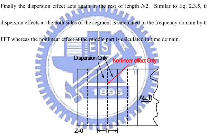
(37) propagate the optical pulse over one segment from z to z+h. In this procedure Eq. 2.3.4 is replaced by z+h. h h A( z + h, T ) ≈ exp( Dˆ ) exp( ∫ Nˆ ( z ' ) dz ' ) exp( Dˆ ) A( z , T ) 2 2 z. (2.3.8). The procedure divides into 3 parts [See Fig. 2.2]. At first, the dispersion effect acts alone in the first half of distance h. Then the effect of nonlinearity acts alone in the middle of segment. Finally the dispersion effect acts again in the rest of length h/2. Similar to Eq. 2.3.5, the dispersion effects at the both sides of the segment is calculated in the frequency domain by the FFT whereas the nonlinear effect at the middle part is calculated in time domain.. Dispersion Only Nonlinear effect Only. A(z,T). Z=0. h. Fig. 2.2 Schematic illustration of the symmetrized split-step Fourier method. Fiber length is divided into a large number of segments of width h. Within the segment, the effect of nonlinearity acts at the midplane shown by a dashed line and the effect of dispersion acts at the edge of the segment shown by a solid line.. 26 .

(38) Because of the symmetric form of Eq. 2.3.8, this scheme is known as the symmetrized split-step Fourier method [43].. The integral in the middle exponential considers the z. dependent of the nonlinear operator Nˆ . If the step size h is small enough, the integral can be approximated by exp( hNˆ ) . The most important advantage of using the symmetrized form of Eq. 2.3.8 is that the leading error term comes from the double commutator in Eq. 2.3.7 is of the third order in the step size h. This can be proved by applying Eq. 2.3.8 twice in Eq. 2.3.7. The accuracy of the symmetrized split-step Fourier method can be further improved by evaluating the integral in Eq. 2.3.8 more accurately than approximating it by hNˆ ( z ) . A simple approach is to employ the trapezoidal rule and approximate the integral by [44] z +h. ∫ Nˆ ( z ) dz '. z. '. ≈. h ˆ [ N ( z ) + Nˆ ( z + h )] 2. (2.3.9). However, the implementation of Eq. 2.3.9 is not simple because Nˆ ( z + h ) is unknown at the mid-segment located at z + h / 2 . It is necessary to use an iterative procedure that is initiated by replacing Nˆ ( z + h ) by Nˆ ( z ) . Equation is than used to estimate A( z + h , T ) which in turn is used to calculate the new value of Nˆ ( z + h ) .. Although the iteration procedure is. time-consuming, it can still reduce the overall computing time if the step size h can be increased because of the improved accuracy of the numerical algorithm. Two iterations are generally enough in practice. Let us see Eq. 2.3.3 again, the nonlinear operator Nˆ contains an integral part and the 27 .

(39) differential part which corresponds to the Raman effect and the SS. It is more complicated to deal with them. We rewrite Nˆ by using Eq. 2.1.6 and Eq. 2.3.3 as the following form: +∞ ⎛ ⎞ 2 2 ˆ N = iγ ⎜⎜ (1 − f R ) A( z,T ) + f R ∫ hR (T ) A( z,T ) dT ' ⎟⎟ −∞ ⎝ ⎠ . +∞ ⎞ ⎫⎪ 1 γ ∂ ⎧⎪ ⎛ 2 2 − ⎨ A ⎜ (1 − f R ) A( z,T ) + f R ∫ hR (T ' ) A( z,T - T' ) dT ' ⎟⎟ ⎬ A ω0 ∂T ⎪⎩ ⎜⎝ −∞ ⎠ ⎪⎭. (2.3.10). The integral part can be solved by the convolution theory by inversely FFT the product of 2. hR (Ω ) (the FFT of hR (T ) ) and the FFT of A( z,T ) [45]. The differential part can be solved in the frequency domain by replacing ∂ / ∂T with iω . Therefore, Nˆ can be written as. γ ⎛ X −1 ⎞ −1 Nˆ = iγX − ⎜ FT [iω FT [ A]] + FT [iω FT [ X ]] ⎟ , ω0 ⎝ A ⎠. {. 2. 2. }. where X = (1 − f R ) A( z, T ) + f R FT−1[hR (Ω ) FT [ A( z, T ) ]] .. (2.3.11). Finally, we can compute the. nonlinear operator Nˆ in use of the convolution theory and the FFT algorithm. In many papers, it is usually solved the SS term using the Runge-Kutta method with treating the differential term as a perturbation [40][45][46]. However, we use the FFT algorithm, which is simpler and more straightforward than the Runge-Kutta method. We therefore simulate the evolution of the pulse spectrum using the split-step Fourier method. We also combine the plug-in program Matfor 4.0 with Compaq Visual Fortran 6.6. Matfor is a very powerful tool which can draft the evolution of spectrum synchronously.. 28 .

(40) 2.4 Verification of the simulations In order to verify accuracy of our simulation, we do some comparisons between the simulation on the paper [18] and ourselves with the same parameters. The first simulated result on Ref [18] is shown in figure 2.3 and the input average power is 16 mW and the pumping wavelength is 800 nm. With the same pumping wavelength, we set the input peak power as 1.6 kW and the pulse width as 100 fs. Then we got the very similar simulated result with the paper in figure 2.4.. Fig. 2.3 The simulated result on Ref[18]. The input average power is 16 mW and the pumping wavelength is 800 nm.. 29 .

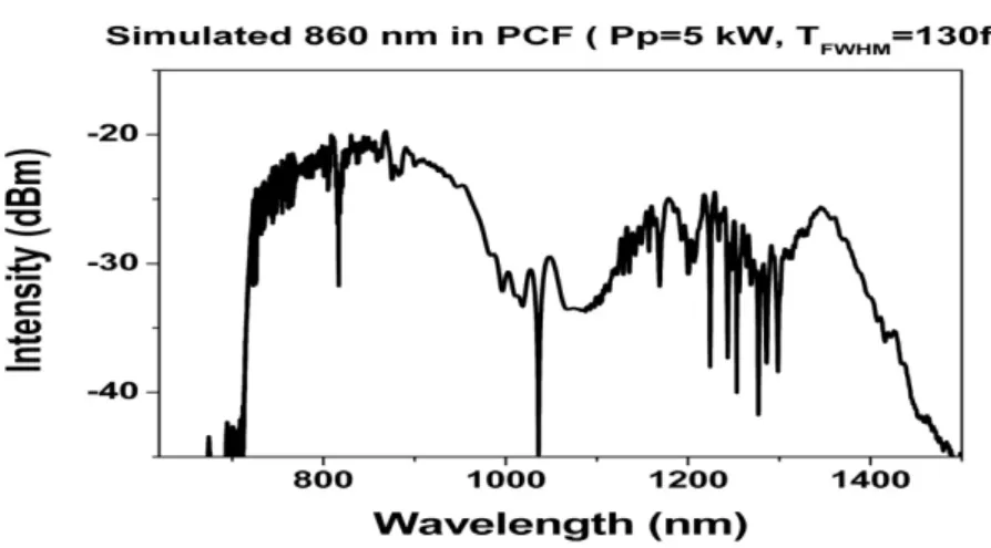
(41) Fig. 2.4 The simulated result by ourselves. The input peak power is 1.6 kW, pulse width is 100 fs and the pumping wavelength is 800 nm. We also compare our simulated result with the reporting result on Ref [18] as shown in figure 2.5. In their simulation, the input average power is 120 mW, TFWHM is 130fs, and the pumping wavelength is 860 nm. We use the same pumping wavelength, pulse width and set the input peak power as 5 kW in our simulation. Our simulated result is shown in figure 2.6 and it is similar to the chart shown in Fig.2.5 (b).. Fig 2.5 SC in 1m of MF: a) measured and b) simulated on Ref[18]. PP=860nm, Pav=120mW, TFWHM=130fs. 30 .

(42) Fig 2.6 The simulated result by ourselves. The input peak power is 5 kW, pulse width is 130 fs and the pumping wavelength is 860 nm. From these two comparisons, we can believe the accuracy of our simulated result and can use this simulation to predict the supercontinuum generation by dual wavelength pumping in the following work.. 31 .

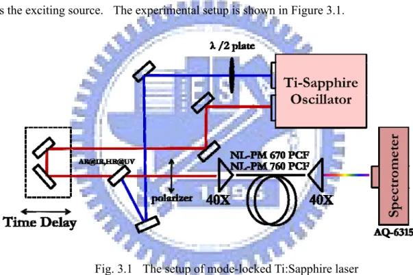
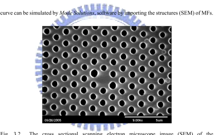
(43) Chapter 3 Experiments. 3.1 Pumping Source The tunable mode-locked Ti:Sapphire laser (from 700 nm to 900 nm, Tsunami, Spectra-Physics inc.) with about 60 fs (FWHM) pulsewidth and 82 MHz repetition rate is used as the exciting source. The experimental setup is shown in Figure 3.1.. Fig. 3.1 The setup of mode-locked Ti:Sapphire laser. 3.2 The Specification of the Used Microstructured Fibers 3.2.1 NL-PM 760 The core diameter of the used microstructured fiber is about 1.7 μm and the pitch Λ (spacing between adjacent holes) is about 1.4 μm.. It is polarization maintaining because of its 32 . .

(44) asymmetric arrangement of the holes near the core.. The diameter of holes is about 0.6μm. except for the two holes near the core whose diameter is about 0.7μm. The cross sectional scanning electron microscope image (SEM) of our MF is shown in Fig. 3.2. This fiber has quite high nonlinearity with nonlinear coefficient γ being 102 km-1⋅W-1 around 800 nm due to its small core diameter. It also has two zero dispersion points which are located at 790 nm and 1190 nm. The used pump wavelength is in the anomalous dispersion region. The dispersion curve can be simulated by Mode Solutions, software by importing the structures (SEM) of MFs.. Fig. 3.2. The cross sectional scanning electron microscope image (SEM) of the microstructured fiber.. 3.2.2 NL-1.5 670 The core diameter of the used microstructured fiber is about 1.5 μm and the pitch Λ (spacing 33 .

(45) between adjacent holes) is about 2.0 μm. The diameter of holes is about 2 μm and the air filling fraction in the holey region is bigger than 90%. The cross sectional scanning electron. microscope image (SEM) of our MF from internet is shown in Fig. 3.3. This fiber has quite high nonlinearity with nonlinear coefficient γ being 168 km-1⋅W-1 at the zero dispersion wavelength due to its small core diameter.. Fig. 3.3. It has only one zero dispersion points at 670 nm.. The cross sectional scanning electron microscope image (SEM) of the microstructured fiber.. 3.2.3 Dispersion Curves of the Microstructured Fibers With a software named Mode Solution, and the relation between the dispersion and the group delay shown as equation (3.1) below,. 34 .

(46) ‫ܦ‬ൌ. ௗఉభ ௗఒ. ,. (3.2.1). where D is dispersion, and β1 is the group delay of this fiber, respectively. We obtained the dispersion curve, group delay and the mode pattern of the photonic crystal fiber NL-PM 760 and NL-PM 670 which are shown in Fig. 3.4 and Fig. 3.5. From Fig. 3.4, two zero dispersion wavelengths can be seen at 790 nm and 1190 nm, but only one zero dispersion wavelength exist at 670 nm as shown in Fig.3.5.. Fig. 3.4 The dispersion curve (black) and the group delay (blue) of the PCF NL-PM 760. The two zero dispersion wavelengths are located at 790 nm and 1190 nm. The inset of this figure is the mode pattern of this fiber.. 35 .

(47) Fig. 3.5 The dispersion curve (black) and the group delay (blue) of the PCF NL-PM 670. The two zero dispersion wavelengths is located at 670 nm.. Then, we calculated phase matching diagram of DFWM from the PCF NL-PM 760. In this process, two pump photons generate one Stokes photon and the other anti-Stokes photon:. 2ω p → ω s + ωas ,. (3.2.2). where ωp, ωs and ωas correspond to the pump, Stokes, and anti-Stokes frequencies, respectively. Being a coherent process, four-wave mixing is efficient only if the phase-matching condition is fulfilled [18], i.e.,. ⎡. Δφ = φ (ωs ) + φ (ωas ) − 2φ (ω p ) = L ⎢2∑ ⎣. n. β 2n. ⎤ (ωs − ω p ) 2 n + 2γPp ⎥ = 0 . (2n! ) ⎦. (3.2.3). Here, β2n is the 2nth derivative of the propagation constant β with respect to the frequency. Base on equation (3.2.3), the FWM diagram of PCF NL-PM 760 and PCF NL-PM 670 are shown below in Fig 3.6 and Fig 3.7. 36 .

(48) Fig. 3.6 Calculated phase-matched wavelengths of PCF NL-PM 760 as a function of pump wavelength through degenerate FMW.. The black line, red line and blue line. correspond to a pump peak power of 0, 0.5, and 3 kW, respectively.. Fig. 3.7 Calculated phase-matched wavelengths of PCF NL-PM 670 as a function of pump wavelength through degenerate FMW.. The black line, red line and blue line. correspond to a pump peak power of 0, 0.5, and 3 kW, respectively. 37 .

(49) 3.3 Experiment Setup of Single and Dual Wavelength Pumping The experiment setup in dual wavelength pumping for SCG is shown in Fig. 3.8. The mode locked Ti:sapphire laser and its second harmonic wave (generated from Model 3980, SP inc.) are simultaneously focused into a 1-m-long MF by a 40X microscope objective lens.. In. this experimental, with about 10% coupling efficiency can be reached. We use a λ/2 plate to change the polarization state of the laser to get the widest spectral broadening, and a polarizer to make sure the same polarization of the fundamental and the second harmonic pulse. Finally, the output spectrum from the PCF is detected and displayed by an optical spectrum analyzer (OSA, Ando).. Fig. 3.8 The setup of our experiment of single and dual wavelength pumping.. 38 .

(50) Chapter 4 Results and Discussion 4.1 Simulated SCG from PCF 4.1.1 Single Wavelength Pumping 4.1.1.1. Fiber NL-PM 760. 4.1.1.1.1 Simulation @ 810 nm Pumping Here, we numerically simulate a SCG from the photonic crystal fiber by using a femtosecond pulse at 810 nm with pulse width about 60 fs. The result is shown in Fig. 4.1. From this figure, the spectrum becomes more and more broadened as the input peak power increases.. Fig. 4.1. The figure shows the simulated evolution of SCG pumped at 810 nm with pulse width equal to 60 fs and different input peak power into the PCF NL-PM 760. The red words show the input peak power, and the green words shows the input average power. 39 . .

(51) 4.1.1.1.2 Simulation with Different Step Lengths The choosing step length in our numerical simulation may slightly result in different broadening spectra.. Therefore, the properly choosing step length in our numerical. simulation is also important.. To make sure the step length in our simulation is acceptable,. we simulated the supercontinuum generation with single wavelength pumping at 810 nm into PCF NL-PM 760 in use of different step lengths.. The experimental observation of the. generated supercontinuum using the pumping wavelength at 810 nm with input average power about 200 mW is shown in Fig. 4.2.. It shows the obviously spectrum dip around. 1380 nm due to the OH- bond absorption.. Fig. 4.2. The SCG pumping at 810 nm with input average power equals to 200 mW. The numerical simulation by using the same pumping wavelength with pulse width equals to 60 fs and input peak power equals to 10 kW is shown in Fig. 4.3. 40 . In the use of the.

(52) step lengths of 1 μm, 5 μm, 10 μm, 50 μm, 100 μm, and 500 μm, the generated SC were shown in Figs. 4.3(a)-(f), respectively.. From these figures, the simulated SC does not. change the shape until the step length less than 10 μm. μm in the following simulation.. Therefore, we use step length of 10. There are few differences between the experimental and the. simulated results in comparing with Fig. 4.2 and Fig. 4.3. The spectrum dip around 1380 nm could not be seen in our simulation because we do not consider the loss due to the OH- bond absorption.. Fig. 4.3. The simulated result of SCG pumped at 810 nm with different step length series. From (a) to (f), the step length are 1 μm, 5 μm, 10 μm, 50 μm, 100μm, and 500 μm, respectively. 41 . .

(53) 4.1.1.2. Fiber NL-1.5 670. In this simulation, the center wavelength and pulse width are 810 nm and 60 fs respectively. In addition, we do not consider the loss term and the high order dispersion (> β3) into our simulation.. The results were shown in Fig. 4.4.. As the input peak power. increases, more Raman solitons are generated and shift toward the longer wavelength.. Fig. 4.4. The figure shows the simulated evolution of SCG pumped at 810 nm with different input peak power into the PCF NL-PM 760. The pulse width is 60 fs. The red words show the input peak power and the green words show the input average power.. 42 .

(54) 4.1.2. Dual Wavelength Pumping with Fiber NL-PM 760. 4.1.2.1. Pumping at Different Wavelength Series. Here, we numerically investigate that dual wavelength femtosecond pulses are simultaneously launched into the PCF NL-PM 760 to generate the SC.. Four sets of. wavelengths are used. They are 760 / 380 nm, 790 / 395 nm, 800 / 400 nm, and 840 / 420 nm, in which they have the same input peak powers and pulse widths. The input peak powers of the fundamental and the second harmonic pulses are both 5 kW.. The pulse width. is 60 fs for the fundamental pulse and 100 fs for the second harmonic pulse, respectively. The simulated results were shown in Fig. 4.5.. We can see that with dual wavelength. pumping, the spectrum become more broadened on the UV side.. The flattest and most. continuous spectrum near the UV side is generated at 790 nm and 395 nm dual wavelength pumping.. The broadened spectrum on the UV side is resulted from the XPM effect.. 43 .

(55) Fig. 4.5. These two figures are the same but with different wavelength range. The figure on the left hand side shows the spectrum on the UV side and the figure on the right hand side shows the whole spectrum. (a)~(d) shows the wavelengths sets of 760 / 380 nm, 790 / 395 nm, 800 / 400 nm, and 840 / 420 nm.. The input peak power of. the fundamental pulse and the second harmonic pulse are both 5 kW.. The pulse. width is 60 fs for the fundamental pulse and 100 fs for the second harmonic pulse, respectively.. 4.1.2.2. Pumping at the Same Wavelength Series but Different Input Peak Powers. In simultaneously use of the wavelength set of 790 / 395 nm as the pump wavelengths, we numerically simulated the spectrum evolution by changing the input peak power that is 44 .

(56) shown in Fig. 4.6. From Figs. 4.6 (a) to (c), the input peak powers are equal to 5 / 5 kW, 7 / 5 kW, and 8 / 8 kW for the fundamental and the second harmonic pulses, respectively.. The. pulse widths of fundamental and the second harmonic pulses are 60 fs and 100 fs, respectively. From Fig. 4.6, the spectra become more broadened and smoother not only on the IR side but also on the UV side as the input peak power increases.. Fig. 4.6. These two figures are the same but with different wavelength range. The figure on the left hand side shows the spectrum on the UV side and the figure on the right hand side shows the whole spectrum.. From (a) to (c), the input peak power are. equal to 5 / 5 kW, 7 / 5 kW, and 8 / 8 kW for the fundamental pulse and the second harmonic pulse, respectively.. The pulse width of fundamental pulse and the. second harmonic pulse are 60 fs and 100 fs, respectively. 45 .

(57) 4.1.3. Comparison of Single and Dual Wavelength Pumping at 790 nm and 395 nm with Fiber NL-PM 760 In Fig. 4.7, we compared the generated spectra in use of the single and dual. wavelength pumping at 790 nm and 395 nm.. The spectrum on the UV side generated in the. use of dual wavelength pumping (black curve) is more broadened than that of using the single wavelength pumping at the second harmonic pulse (blue curve), and that is due to the XPM effect between the fundamental and the second harmonic pulses. (a). Fig 4.7. (b). The simulated result of single and dual wavelength pumping at 790 nm and 395 nm on PCF NL-PM 760.. (a) shows the spectrum on the UV side and (b) shows the. whole spectrum. The black curve is dual wavelength pumping, red curve is single wavelength pumping at 790 nm and blue curve is single wavelength pumping at 395 nm.. The input peak power and pulse width of 790 nm are 7 kW and 60 fs.. input peak power and pulse width of 395 nm are 5 kW and 100 fs.. 46 . The.