利用量子球檯介觀波函數類比研究大面積面射型雷射之橫向模態

國

立

交

通

大

學

電子物理學系

博

士

論

文

利用量子球檯介觀波函數類比研究大面積面射型雷射

之橫向模態

Analogous Investigations on the Transverse Modes of Broad-Area

Vertical-Cavity Surface-Emitting Lasers by Mesoscopic Wave

Functions of Quantum Billiards

研 究 生：陳建誠

指導教授：陳永富 教授

Analogous Investigations on the Transverse Modes of Broad-Area Vertical-Cavity

Surface-Emitting Lasers by Mesoscopic Wave Functions of Quantum Billiards

研 究 生：陳建誠 Student：Chien-Cheng Chen

指導教授：陳永富 Advisor：Yung-Fu Chen

國 立 交 通 大 學

電 子 物 理 學 系

博 士 論 文

A Dissertation

Submitted to Department of Electrophysics College of Science

National Chiao Tung University in partial Fulfillment of the Requirements

for the Degree of Doctor of Philosophy

in Electrophysics

June 2009

Hsinchu, Taiwan, Republic of China

學生：陳建誠 指導教授：陳永富

國立交通大學電子物理學系博士班

摘

要

近軸近似光學與二維量子力學之間的類比性是本篇論文的核心概念。基

於 Helmholtz 方程式與非時變 Schrödinger 方程式之間的相似性，我們可以用

量子球檯的介觀波函數解釋大面積面射型雷射的高階近場橫向模態。相反

地，非可積量子球檯的波函數雖然沒有解析解，但我們可以利用混沌形狀的

面射型雷射做類比觀察。除此之外，同調波突然從量子球檯釋放出來之後的

演變也可以透過面射型雷射之橫向模態的傳遞做類比觀察。由於二維量子系

統與近軸光學的類比性不僅止於波函數與橫向模態，還包括它們的軌道角動

量，所以藉由計算同調波從量子球檯釋放出來之後的軌道角動量可以類比分

析面射型雷射光束的軌道角動量。更有趣的是，面射型雷射的模態除了線性

偏振之外，還可以形成一種偏振與空間糾纏的向量場。既然光的偏振乃是對

應於量子波的自旋，分析面射型雷射之中的向量場可以提供重要的資訊給考

慮電子自旋的量子球檯系

統。

Student：Chien-Cheng Chen Advisor： Yung-Fu Chen

Department of Electrophysics

National Chiao Tung University

ABSTRACT

The analogies between paraxial optics and two-dimensional (2-D) quantum mechanics lie in the heart of this thesis. Based on the similarity between Helmholtz equation and time-independent Schrödinger equation, mesoscopic wave functions of quantum billiards are used to interpret the high-order transverse modes of broad-area Vertical-Cavity Surface-Emitting Lasers (VCSELs). Reversely, chaotic-shaped VCSELs can be employed to analogously observe the wave functions of non-integrable billiards which have no analytic solutions. In addition, the free-time evolution of coherent waves suddenly released from quantum billiards can be analogously observed from the free-space propagation of lasing modes emitted from VCSELs. Furthermore, the analogies are not restricted to quantum wave functions and optical transverse modes, the orbital angular momentum (OAM) density carried by a light beam emitted from VCSELs can be analogously analyzed by calculating the OAM of coherent waves abruptly set free from quantum billiards. More interestingly, the lasing modes of VCSELs are not only linearly-polarized but can form the vector fields, in which the polarization is spatially dependent. Since the polarization of light corresponds to the spin of quantum wave, the analyses of the vector fields in VCSELs can provide important information for quantum-billiard systems (such as ballistic quantum dots) with consideration on electronic spin.

首先要感謝我的指導教授陳永富老師。以前每當有人問起誰是影響自己最多的人時， 心裡總是沒有明確的答案。但現在我可以肯定的說，是陳永富教授。讀大學時候的我根本 沒想過會攻讀博士，但機緣之下陳老師讓我得以一窺科學的美妙。從一開始用挖洞的方法 重建 Chaotic Patterns 我就已經著迷於這神奇的世界，後來種種的實驗發現與理論計算重建 都一次一次的撼動我的心，我也常常為了這些發現而興奮好幾天。雖然我在研究過程中常 常讓老師失望，但老師還是一直很有耐心的指引我，把我導向正途。陳老師讓我成長的並 不僅止於學識，老師的言教身教也歷歷在在地影響我的人生觀，讓原本避世的我也想要成 為跟老師一樣熱血有抱負的人。能夠讓我完成博士學業的另一隻推手是跟陳老師共同指導 我的黃凱風教授，黃老師提供了世界一流的實驗設備及元件，讓我可以無憂無慮的做研 究。此外，黃老師淵博的學識與對科學的熱誠是我所景仰的，每當碰到瓶頸黃老師總是可 以指點我明確的方向找到出口。除此之外，聽黃老師講故事是非常享受的。在這段日子有 兩位良師可以一起教導我、帶我探索充滿驚奇的科學世界讓我感到萬分幸福。往後的日子 裡，我將效法兩位恩師的精神，孜孜不倦地為科學貢獻一己之力。 除了老師之外，首先要感謝蘇冠暐老大帶我做研究，你的認真、細心、及觀察力一直 是我的學習指標。在實驗器材上，要感謝洪天河先生不厭其煩的鼎力相助。另一方面要感 謝劉春鞠學姊帶我整理研究工作，跟你的討論使我受益良多。感謝陸亭樺學姊，黃哲彥、 黃仕璋、王偉立學長，有你們做為學習的榜樣，我才能真正融入研究生活。當然還有一起 奮鬥成長的興弛、依萍、雅婷、恩毓，有你們一起修課、討論作業、互相砥礪，讓我享受 跟朋友一起學習的愉快。此外彥廷、建至、阿仁，跟你們討論幫助我釐清很多觀念。另外， 蔡玲意及古美玲學姊、黃國欽及林伯祥學長、阿龍哥、黃文政、紀暐、李易純、陳毅帆、 莊威哲、龔家禎、林毓捷雖然跟大家只有短暫的相處，但我感覺得出來你們都是好人。還 要額外感謝一起打球的好伙伴梁興弛、偉立哥、彥廷、阿仁，雖然我打球只有一千零一招， 但有你們的強大支援還是可以讓我在短短的時間內有充足的運動量。除了實驗室的夥伴之 外，我要感謝光環科技公司提供各種雷射元件，也感謝口試委員的指正與建議。 感謝跟我同甘苦共患難的老婆宸聿這麼多年來的陪伴，你跟宣竹是我認真向上的動 力。還有感謝哥哥姊姊們對我從小的照顧與疼愛。最後，僅以此文獻給我摯愛的雙親，特

Abstract (Chinese) ………... i Abstract ………... ii Acknowledgement ………... iii Contents ………... iv List of Figures ………... vi Chapter1 Introduction………..………..………. 1 1.1 Quantum Billiards……… 2 1.2 Diffraction in Time……….. 6

1.3 Singularities in Optical Waves……… 10

1.4 Vertical-Cavity Surface-Emitting Lasers……… 18

1.5 Overview of Thesis………...……… 24

Chapter2 Wave Functions of Quantum Billiards………. 26

2.1 The Square Billiard………... 27

2.2 The Equilateral-Triangular Billiard………..……… 36

2.3 The Chaotic Billiards……….………... 47

Chapter3 Analogous Observation on Quantum-Billiard Wave Functions from VCSELs……….. 56

3.1 The Analogy between VCSELs and Quantum Billiard…….……... 58

3.2 Experimental Sutup………... 61

3.3 Typical Lasing Modes of Square VCSEL……… 64

3.4 Chaotic Wave Function in Rippled-Square VCSEL………. 73

4.1 Stationary States Suddenly Released from 1-D Infinite Potential

Well………... 100

4.2 Transient Dynamics of Coherent Waves Released from Quantum Billiard……….. 104

4.3 Analogous Observations on Coherent Waves Released from Quantum Billiard by Free-Space Propagating Transverse Modes of VCSELs……… 112

4.4 Probability Current and Angular Momentum Densities of Coherent Waves Released from Quantum Billiard: Optical Vortices Generated by VCSEL………. 118

Chapter5 Vector Fields and Vector Singularities in VCSELs………. 145

5.1 Vector Field in Square VCSEL………. 147

5.2 Chaotic Vector Field in VCSE……….. 156

Chapter6 Summary and Future Work……….. 167

6.1 Summary………... 168

6.2 Future Work……….. 171

Appendix A Diffraction in Time: Moshinsky’s Shutter Problem……...……. 172

Appendix B Angular Momentum Density of a Light Beam………. 176

References ……….. 182

Curriculum Vitae ………... 201

Chapter1

Fig. 1.1-1. Schematic diagram for a 2D flat billiard. The particle in the billiard goes in straight lines. The incidence angle on the wall equals the reflection angle. The energy of the particle is constant.

Fig. 1.2-1. (a) Demonstration of the shutter problem. (b) Red curve displays the temporary interference pattern and blue dash line indicates a classical result. (See Appendix A for a more detailed discussion.)

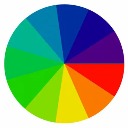
Fig. 1.3-1. A color wheel. At the center the color becomes undefined.

Fig. 1.3-2. (a)-(b) Vector fields with vortex, saddle, and source, respectively; (a’)-(b’) The corresponding orientation angle function of vector fields shown in (a)-(b).

Fig. 1.3-3. (a)-(c) The phase structures of singularities, saddle, and maximum (extremum). The gradient of these phases will result in the vector fields shown in Fig. 1.3-2 (a)-(c), respectively.

Fig. 1.4-1. Schematic diagram of an edge-emitting laser. The laser output is parallel to the semiconductor layers. The out put beam is highly diverged due to the thin emission region.

Fig. 1.4-2. Schematic diagram of a VCSEL. The laser output is perpendicular to the

wafer. The isotropic aperture results in a good beam quality.

Chapter2

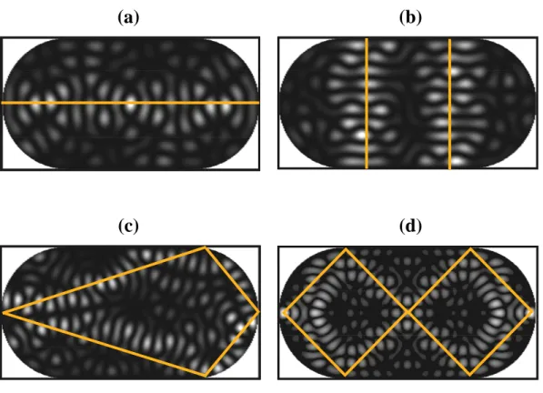
Fig.2.1-1. Some classical periodic orbits denoted by ( , , )p q , where p and q are two positive integers describing the number of collisions with horizontal and vertical walls, and the parameter  (   ) that is related to the wall    positions of specular reflection points.

Fig.2.1-3. Stationary coherent states _50,20p q, ,( , )x y associated with classical periodic orbits ( , , )p q .

Fig.2.1-4. The N dependence of the wave pattern . It can be seen that N is related to the mode order.

1,1,0.6 2 ,5 |CN ( ,x y  ) | ) |

Fig.2.1-5. _{The M dependence of the wave patterns . It can be seen}

that M is related to the localization of the patterns.

1,1,0.6 2 30,

|C _M( ,x y

Fig.2.2-1. Some classical periodic orbits ( , , )p q  , where p and q are two positive

integers with restriction p , and the parameter q  (   ) is   

related to the initial point of the billiard ball.

Fig.2.2-2. _{Some eigenstate of equilateral-triangular billiard} ( ) , ( , )

C m n x y

 .

Fig.2.2-3. _{Some eigenstate of equilateral-triangular billiard} ( ) , ( , ) S m n x y  . Notice that . ( )S | 2 ,n n( , )x y 0  

Fig.2.2-4. _{Stationary coherent states} 2 50,15

|Tri ( , ; , , )x y p q associated with classical periodic orbits ( , , )p q  .

Fig.2.2-5. _{The N dependence of the wave pattern . It can be}

seen that N is related to the mode order.

2 ,10

|CTri_N ( , ;1, 0,x y / 3)|

|

Fig.2.2-6. The M dependence of the wave patterns . It can be seen that M is related to the localization of the patterns.

2 40,

|CTri_M( , ;1, 0,x y / 3)

Fig. 2.3-1. The stadium billiard. The trajectory in chaotic billiard is generally ergodic. Fig. 2.3-2. Some unstable periodic orbits in the stadium billiard.

Fig. 2.3-5. (a) A random superposition of several eigenstates with quantum number

satisfying 54 n12n22 55, as illustrated in (b)

Fig. 2.3-6. (a)-(b) The statistics for the amplitude and intensity of the random wave shown in the previous figure. The fitting curves are Gaussian and Porter-Thomas distributions, respectively.

Fig. 2.3-7. (a)-(d) The scars appear in the 122nd, 132nd, 207th, and 258th exited states of the slightly asymmetric stadium billiard. The highlighted lines indicate the unstable periodic orbits.

Chapter3

Fig.3.1-1. (a) The schematic diagrams for vertical-cavity surface-emitting laser. he separability of the wave function in the VCSEL device enables the wave vectors to be decomposed into kz and kt. (b) The illustration of a wave a

wave incident upon the current-guiding oxide boundary would undergo total internal reflection for k_t  k_z.

Fig.3.2-1. The schematic diagrams for the experimental setup.

Fig.3.2-2. (a) The VCSEL mounted on the copper holder. (b) Side view of the

cryogenic system. (c) The objective lens with NA=0.9 (d) Face view of the cryogenic system.

Fig. 3.3-1. The SEM image of square VCSEL device

Fig. 3.3-2. Optical microscope image view from the aperture of the VCSEL. The bright region display the spontaneous emission to manifest the details on the square boundary.

Fig. 3.3-3. (a) The temperature dependence of the threshold current and the lasing modes observed at temperatures of (b) 295K (room temperature) (c) 285K (d) 250K (e) 230K.

1,1,0.57 1,1,0.46 y  1,1,0.8 y  K

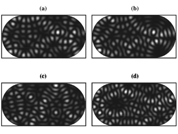
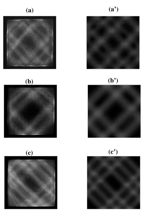
Fig. 3.3-5. a)-(c) Various superscar modes observed in different square VCSEL devices. (a’)-(c’) Theoretical interpretation of (a)-(c) by SU(2) coherent states C_36,10 ( , )x y , C_38,6 ( , )x , and C_40,25 ( , )x respectively

Fig. 3.3-6. (a)-(c) Various multi-POs superscar modes observed in different square VCSEL devices. (a’)-(c’) Theoretical patterns of (a)-(c) given by Eq. (3.3.6)-(3.3.8), respectively.

Fig. 3.4-1. Experimental pattern of the spontaneous emission to manifest the details on the ripple boundary.

Fig. 3.4-2. Near-threshold lasing patterns of the rippled VCSEL at temperatures of (a)T260 and (b)T220K.

Fig. 3.4-3. (a) An unknown wave function (b) The intensity distribution (c) Square Root of intensity distribution (d) Positive part of the wave function (e) Demonstration of 2_p( ) |x  ( )x | (f) The result of 2_p( ) |x  ( ) |x .

Fig. 3.4-4. (a) and (b) The intensity plots of the positive wave functions | p(xi, yj)| for experimental results shown in Figs. 3.4-2 (a) and (b), respectively.

Fig. 3.4-5. (a) and (b) Distribution of the coefficients obtained by Eq. (3.4.6) for experimental results shown in Figs. 3.4-1 (a) and (b).

,

|C_{m n}|

Fig. 3.4-6. (a) and (b) The reconstructed patterns with the eigenfunction expansion method for experimental results.

Fig. 3.4-7. (a) and (b) Tthe amplitude distributions of the wave functions shown in Fig. 3.4-6 (a) and (b), respectively.

Fig. 3.4-8. (a) and (b) The intensity distributions of the patterns shown in Fig. 3.4-6 (a) and (b), respectively.

|

S

tr.iangular VCSEL.

Fig. 3.5-3. (a)-(i) The near-threshold lasing patterns of triangular VCSEL at temperatures labeled by A-I in Fig 3.5-2, respectively.

Fig. 3.5-4. (a) Experimental pattern observe at 195K. (b) Numerical wave pattern of eigenstate |( )_5,55( , )x y 2.

Fig. 3.5-5. Experimental pattern observe at (a)275K and (b)135K; Numerical wave pattern of coherent state (c) |C_{36, 9}Tri ( ,x y; 1, 0, 0.23 ) | 2 and (d)

2

Tri

20, 6

|C ( ,x y ; 1, 1, 0.35 ) | ; The classical periodic orbits that the wave functions localized on are depicted in the insets of (c) and (d).

Fig. 3.5-6. The intensity plots of the positive wave functions | p(xi,yj) | for experimental results shown in Figs. 3.5-3 (f).

Fig. 3.5-7. (a) Experimental pattern observe at 175K. (b) Reconstructed pattern of (a). (c) Intensity statistics of (b) with fitting curve to be Porter-Thomas intensity distribution.

Chapter4

Fig. 4.1-1. _{(a)-(k) Intensity plots of} S_{( , ;10)}

x t

 at t 0T-T , respectively, with equal

time interval  t 0.1T . (l) Intensity plots of ₁₀( , )x t at t . The intensity pattern preserves its shape after

1.5T

t1.5T .

Fig. 4.2-1. _{Numerical patterns to illustrate the wave patterns} 2 15,15( , , )x y t  at t = (a) , (b) , (c) , (d) , (e) , (f) , (g) , (h) , and (i) . 0T 2.0 T 1 . 0 0.2 T 0.3 T 0.4 T 0.5 T 1.0T T

Fig. 4.2-2. _{Numerical patterns to illustrate the wave patterns 1,1,0.6} 2 35,13 ( , , )x y t

 at t =

(a) , (b) , (c) , (d) , (e) , (f) , (g)

, and (i) .

, and (i) . 2.0 T

Fig. 4.2-4. _{Numerical patterns to illustrate the wave patterns} 2

( , , ) chaos x y t  at t = (a) , (b) (c) , (d) , (e) , (f) , (g) , (h) , and (i) . 0T 3.0 T 1 . 0 , 0.2 T 0.4 T 0.55 T 0.8 T 1.5 T T

Fig. 4.3-1. Experimental patterns of a superscar mode with propagation distance at z =

(a) , (b) , (c) , (d) , (e) , (f) , (g)

, (h) , and (i) 20cm, where

0z_d d z 0.1 z_d 2.0 z_d 0.2 z_d 0.3 z_d ~ d 0.4 z_d z m 0.7 z_d 1.0 72 .

Fig. 4.3-2. Experimental patterns of a chaotic mode with propagation distance at z = (a)

, (b) , (c) , (d) , (e) , (f) , (g) ,

(h) , and (i) 20cm, where

0z_d 0.1 z_d d z 0.2 z_d 0.4 z_d ~ 1 d 0.55 z_d z m 0.8 z_d 1.5 z_d 3.0 38 .

Fig. 4.4-1. (a)-(f) The vector plot of j_15,15( , , )x y t at t0.1T , , , ,

, and , respectively.

0.2T 0.3T 0.4T

0.5T 1.0T

Fig. 4.4-2. _{(a)-(f) show the density plots of}

15,15( , , )

l x y t at t0.1T, , ,

, , and , respectively.

0.2T 0.3T

0.4T 0.5T 1.0T

Fig. 4.4-3. The OAM spectrum of _15,15( , , )x y t .

Fig. 4.4-4. _{(a)-(f) The vector plot of} 1,1,0.6

35,13 ( , , )

J  x y t at t0.1T , , ,

, , and , respectively.

0.2T 0.3T

0.4T 0.5T 1.0T

Fig. 4.4-5. _{(a)-(f) The density plots of} 1,1,0.6

35,13 ( , , )

L  x y t at t 0.1T , , ,

, , and are presented in Fig. 4.3-9 (a)-(f), respectively.

0.2T 0.3T

0.4T 0.5T 1.0T

Fig. 4.4-6. _{The OAM spectrum of} 1,1,0.6

35,13 ( , , )x y t 

 .

Fig. 4.4-7. _{(a)-(c) The intensity patterns of} 1,1,

35,13( , , )x y t 

 with   , 0 0.25 , and

Fig. 4.4-9. (a)-(f)The density plots of 1,1,0.6 35,13 ( , , ) Lc  x y t at t0.1T , , , , , and , respectively. 0.2T 0.3T 0.4T 0.7T 1.0T

Fig. 4.4-10. The OAM spectrum of 1,1,0.6 .

35,13 ( , , ) C  x y t

Fig. 4.4-11. (a)-(f) The vector plot of j_chaos( , , )x y t at t 0.1T , , ,

, , and , respectively.

0.2T 0.4T

0.55T 0.8T 1.55T

Fig. 4.4-12. (a) The vector plot of j_chaos( , , 0.1 )x y T . (b)-(d) Zoom-in views of small regions marked by the hollow squares in (a). Backgrounds are the corresponding contour plots of phase functions.

Fig. 4.4-13. (a) The vector plot of j_chaos( , , 0.2 )x y T . (b)-(d) Zoom-in views of small regions marked by the hollow squares in (a). Backgrounds are the corresponding contour plots of phase functions.

Fig. 4.4-14. (a) The vector plot of j_chaos( , , 0.4 )x y T . (b)-(d) Zoom-in views of small regions marked by the hollow squares in (a). Backgrounds are the corresponding contour plots of phase functions.

Fig. 4.4-15. (a)-(f) The density plot of l_chaos( , , )x y t at t 0.1T , , ,

, , and , respectively.

0.2T 0.4T

0.55T 0.8T 1.55T

Fig. 4.4-16. The OAM spectrum of _chaos( , , )x y t .

Chapter5

Fig. 5.1-1. (a) Reference of the polarization angle (b) The threshold currents of the two polarizations. Simultaneous lasings occur at temperatures around

and .

295K 255K

Fig. 5.1-2. (a)-(d) The lasing patterns in 0, 45, 90, and 45 and (e) The total intensity pattern observed at 295K.

Fig. 5.1-5. (a) The contour plot of the angle function ( , )x y . (b) Zoom-in view of the small regions highlighted by the white square. (c) The vector plot of the polarization vector with vortices and saddles labeled by “＋” and “－” signs, respectively.

Fig. 5.2-1. Experimental polarization-resolved near-field patterns observed at the operating temperature of T=265 K with polarization in (a) 0°(perpendicular) (b) 90° (horizontal) (c)45° (d)135°.

Fig. 5.2-2. (a) and (b) Intensity plots of the positive wave functions | p(xi,yj)| for experimental results shown in Figs. 5.2-1(a) and 5.2-1(b), respectively.

Fig. 5.2-3. (a) and (b) Distribution of the coefficients obtained by Eq. (3.4.6) for experimental results shown in Figs. 5.2-1(a) and (b), respectively.

,

|C_{m n}|

Fig. 5.2-4. (a)-(d): Reconstructed patterns with the eigenfunction expansion method for experimental results shown in Fig. 5.2-1(a)-(d), respectively.

Fig. 5.2-5. Amplitude distributions of the polarization-resolved wave functions (blue step lines) for experimental results shown in Fig. 5.2-1(a)-(d), respectively. Red lines: Gaussian distributions (Eq. (2.3.2)).

Fig. 5.2-6. Intensity distributions of the polarization-resolved wave functions (blue step lines) for experimental results shown in Fig. 5.2-1(a)-(d), respectively. Red lines: Porter-Thomas distributions (Eq. (2.3.3)).

Fig. 5.3-7. (a) The contour plot of the angle function _C( , )x y . (b)-(c) Zoom-in view of the two small regions with the hollow circles on the singularities.

Chapter 1

Introduction

1.1 Quantum Billiards

Billiards is known as a dynamical system in which a particle goes in straight line and elastically reflects from the hard-wall boundary, as illustrated in Fig. 1.1-1. In general the region enclosed by the boundary of the billiards can be multi-dimensional and even in non-Euclidean space [KL91], but here subject is restricted to the billiards in two-dimensional (2D) plane. Depending on the initial conditions, initial position and velocity, there are infinitely possible trajectories and they are all deterministic, i. e. they can be traced. Besides, the Poincare map of the billiards can be easily obtained by calculating particle’s incident angle on the circumference. As a result, billiards is often used as a paradigm in study chaos [Sina70, Buni79].

Quantum billiards [Stöc99], a quantum analogue of classical dynamic billiards, is actually a 2D infinite potential well in arbitrary shape. According to Bohr-Sommerfeld quantization rule, the eigenenergies of the quantum billiards can be calculated from the classical periodic orbits (POs). In 1917 Einstein suggested that the close integral in Bohr-Sommerfeld quantization rule can be evaluated in phase space in which the energy surface of an integrable system forms a torus [Enge97, Ston05]. Meanwhile, Einstein raised a question: how to quantize a classically nonintegrable system, since there is no close loop in phase space. The survey concerns the quantum manifestation of classical chaos was then termed quantum chaos [BÅ00, Stöc99] or quantum chaology [Berr87].

Even though quantum mechanics has been well developed in 1920s, Einstein’s question was not answered until Gutzwiller used trace formula to connect the quantum mechanical energy density with classical POs of chaotic systems in 1970s [Gutz71, Gutz80, Gutz90]. The periodic-orbit theory has been experimentally tested by microwave billiards [SS90, Rich01]. Furthermore, the periodic-orbit theory was utilized to show that the statistics of nearest-neighbor energy spacing of chaotic system should obey Wigner distribution, in contrast to Poisson distribution of regular

system [Berr83]. This level statistics is often used as a signature of quantum chaos and has been intensively studied in quantum billiards [MK79,SS90] as well as in other various systems [DG86, Haak91, Wint87, WKL+89].

On the other hand, the wave-function aspect, Berry used semiclassical approach to show that the autocorrelation function of chaotic wave function is Bessel-type and suggested that chaotic wave function should be Gaussian random waves [Berr77]. With the numerical computation, this conjecture was validated by McDonald and Kaufman who showed that the eigenfuntion of stadium billiard indeed exhibits random pattern [MK79, MK88]. Although the chaotic eigenfunctions were shown to be generally ergodic, Heller showed that high-order eigenfunctions of stadium billiard would concentrate on the classical unstable periodic orbits [Hell84]. Such a localized wave function has been called the “scar [Hell84].”

The scar has been shown to play a vital role in a wide variety of physical systems. For examples, the lasing mechanism of high-power directional emission in deformed microdisk lasers has been analogously interpreted with the scar effect in chaotic billiards [GCN+98, LLHZ06, LLZ+07, NS97, NSC94, RTS+]; the conductance fluctuations of quantum dots, in which electronic motion is predominately ballistic in nature, have also been shown to be closely related the scarred wave functions [BAF+99]; the efficiency of fiber laser can be enhanced by selectively amplification of scarred optical wave [MDLM07].

Even if the scar has been shown to be very important, direct experimental observation of scarred matter wave is very few [CSG+03] since the wave function of 2D system is very difficult to measure. The observations of the scar were mostly performed in analogous experiments. Due to the analogy between 2D Helmholtz equation and 2D time-independent Schrödinger equation, the first experimental visualization of scars was realized in the microwave cavity [KKS95, Srid91, SS92]. As well as microwave cavity, scar modes were also manifested in acoustic wave cavity [CH96, KAG01,]. Besides, the scarred optical patterns were also shown to appear in the transverse mode of optical fiber [DLM01].

superscars [BS04, BDF+06]. The terminology “superscar” was originally used by Heller [Hell84] to refer the wave functions localized on stable periodic orbits in stadium billiard and to make a difference with scar. Recently its meaning was extended to wave function localized on stable periodic orbits in pseudointegrable billiard [BS04, BDF+06]. Superscar has also been shown to closely relate to the conductance fluctuation of quantum dots [AF99, CLO+97, LMH+06] and the mode characteristics of microdisk lasers with regular shapes [AYL+06, CKH+00, HGW00, HGYL01, LCG+04, PCC01, YAK+07]. However the analogous observations of the superscars are much fewer than that of scars [BDF+06, HCLL02]. The main aim of this thesis is to analogously observe the superscar mode by broad-area vertical-cavity surface emitting lasers (VCSELs) [HCLL02, CHLL03a, CLS+07, CSCH08]. Besides, the coherent states to describe the superscars in square and equilateral-triangular billiards will be developed [CH03, CHL02].

Fig. 1.1-1. Schematic diagram for a 2D flat billiard. The particle in the billiard

goes in straight lines. The incidence angle on the wall equals the reflection angle. The energy of the particle is constant.

1.2 Diffraction in Time

Diffraction is a particular behavior of waves, which occurs when propagating waves encounter obstructions. It may results in a digression from the geometrical path including deflection into geometrically forbidden regimes. As well as classical waves (such as light, sound, or water waves), matters (such as electron, neutron, or proton) can also be diffracted due to wave-particle duality [DG27, SWMD48, WS48]. The diffraction mentioned above are spatial, while Moshinsky showed that matter wave can be also diffracted in time [Mosh52], i. e. waves can be deflected into a time zone which is classically prohibited. Consider the following shutter problem proposed by Moshinsky: A monochromatic non-relativistic particle beam, moving

parallel to the x-axis, incidents on a completely absorbing shutter placed at ,

as illustrated in Fig. 1.2-1 (a). If the shutter is suddenly opened, what will be the transient particle current observed at a distance behind the shutter? By the analogy between paraxial optics and non-relativistic quantum mechanics [DD04], it was showed that the transient wave function has remarkable temporary interference pattern (as shown in Fig. 1.2-1 (b)) analogous to the spatial interference pattern of light diffracted by a sharp edge [Mosh52] (See Appendix A for a more detailed discussion). Since Moshinsky first put forward this idea, diffraction in time has received considerable attentions. The time evolution of various bound states [Godo02, Godo03] and even arbitrary initial conditions [GM05] have been investigated for an abrupt potential change. Besides, the transient dynamics has also been studied for potentials with different time modulations [dCMM07]. Moreover, the case of matter wave diffraction simultaneously in space and time has also been considered [BZ97]. The experimental test for this diffraction-in-time effect was indeed hard to reach at the time of the first introduction. However, due to the development in ultrafast laser [PLW+03], atom cooling, and optical trapping [WPW99], the transient dynamics has been recently observed in wide variety of

0

systems including neutrons [HFG+98], ultracold atoms [SSDD95], electrons [LSW+05], and Bose-Einstein condensates [CMPL05].

The explorations of diffraction in time are not only for scientific interests but also have some potential applications, as the transient response to abrupt changes of the confined potential in semiconductor structures and quantum dots would exhibit diffraction-in-time effect [DCM02, DMA+05]. As indicated in previous section, semiconductor quantum dots have been widely used as 2-D quantum billiards to explore the properties of quantum chaos [NH04]. Understanding the time evolution of suddenly released quantum-billiard waves can provide the nanostructure transport properties for developing novel ultrahigh-speed semiconductor devices [DCM02, DMA+05]. Moreover, it is closely related to atom laser dynamics from a tight wave guide whose boundary shape can be modified with the laser-trapping beam [dCL+08]. However the presented theoretical analysis only focuses on 1D potential barrier, the diffraction in time of 2D quantum-billiard wave functions has never been explored. In 1-D systems the current flow is monotonous since it is linear and can only flow to

two direction, x or x axes. However, the 2-D probability current density

becomes much complicated because its multi directionalities. Moreover, orbital angular momentum (OAM), which is an important physical quantity both in classical- [GPS02] and quantum-mechanical [BVD65] systems, will naturally arise due to the 2D current flow.

In this dissertation, the time evolutions, probability currents, and OAM densities of eigenstate, coherent state, and chaotic state released from 2D square billiard are theoretically investigated. Besides, the evolution of the time-diffracted wave functions are analogously observed by the free space propagation of lasing modes of VCSEL based on the similarities between paraxial optics and non-relativistic quantum mechanics. However, the analogies between paraxial optics and 2-D quantum system are not only restricted to the correspondence between amplitude distribution and wave function but also consist in the similarity between optical and quantum OAM densities [ZB06, ZB07]. Recent years have been increased attention being given to optical OAM [ABSW92, FAAP08] for its wide applications in atom trapping

[KTS+97], optical tweezers [MRS+99], and optical spanner [SADP97]. Furthermore, OAM of light beam can be encoded as qudit and has great potential applications in quantum information [MVWZ01]. Therefore, the analysis on quantum OAM of wave functions released from 2D billiard can be served as an analogous investigation on optical OAM of lasing modes emitted from VCSEL.

(a)

(b)

x

0

0 1 2 3 4 5 6 7 8 9 10 0 1 2 ( ) t T ( )t 0 1 2 3 4 5 6 7 8 9 10 0 1 2 0 1 2 3 4 5 6 7 8 9 10 0 1 2  ( ) t T ( )t 

Fig. 1.2-1. (a) Demonstration of the shutter problem. (b) Red curve displays

the temporary interference pattern and blue dash line indicates a classical result. (See Appendix A for a more detailed discussion.)

1.3 Singularities in Optical Waves

Singularities are places at which some quantities become undefined. For example, as shown in Fig. 1.3-1, the center of a color wheel is a color singularity at which the color becomes undefined. The basic reasons study singularities is because of their ubiquity and structural stability [Berr80]. For optical waves, there are mainly two kinds of singularities being concerned: phase singularities and polarization singularities [Nye99]. The survey of these singularities has becomes a very modern area of interest in contemporary physics and is named singular optics [SV01].

Generally, phase singularities [Berr98] are points in plane and lines in space at which intensity vanishes and the phase of complex scalar wave field become undefined. In this work only 2D complex scalar field is concerned, which stand either for 2-D quantum wave function or for transverse modulus of light beam. It is convenient to introduce the mathematical form

( , )x y R x y( , ) i I x y ( , )

   . (1.3.1)

with R x y and ( , )( , ) I x y to be real. By defining ( , )x y R x y2( , )I2( , )x y and ( , )x y arg[ ( , )] x y , the scalar field can rewrite as

( , )x y  ( , ) exp[ ( , )]x y i x y . (1.3.2) The positions at which R x y and ( , )( , ) I x y simultaneously equal to zero such that the amplitude ( , )x y vanishes and the phase ( , )x y becomes undefined are the phase singularities. These nodal points in 2D plane are analogous to crystal dislocation and are also referred as phase dislocation [NB74].

which is generally given by * ( , ) Im[ ( , ) ( , )] j x y x y x y m       . (1.3.3)

Substituting Eq. (1.3.2) in to Eq. (1.3.3), the probability current density can be alternatively expressed as the gradient of the phase ( , )x y

( , ) ( , ) ( , ) j x y x y x y m      . (1.3.4)

According to fundamental calculus, the curl of j will be zero at all positions except for the phase singularities. Hence, phase singularity is also termed as vortex for the circulating current density around it. The vortices have been involved in a wide variety of coherent phenomena such as superconducting films [MFDM03], superfluid [MFDM03], Bose-Einstein condensate [MAH+99], microwave billiards [ŠHK+97], quantum ballistic transport [BSS02], and liquid crystal films [dGP93].

One important characteristic of a phase singularity is its topology charge (also named as winding number or dislocation strength) defined by

1 1 ˆ ( , ) ( ) 2 _C 2 _C x ˆy s d  x y dx a dy   

_





_



   a (1.3.5)

, where C is arbitrary closed loop containing only one singularity inside. The

charge is positive (negative) if the phase circulates counterclockwise (clockwise). A crucial topological property of singularities is the sign rule which indicates that the charge of the neighboring singularities on a constant phase contour must have opposite signs [Freu95].

Due to the underlying analogy between optical momentum density and the probability current density (See Appendix B for a more detailed discussion), the phase singularity of the amplitude distribution of light beam manifest itself as optical vortex

[VS99]. Consequently, optical vortices is intimately related to optical OAM [SGV+97]. As revealed in last section, optical OAM has attracted much interest because of the wide applications, such as atom trapping [KTS+97], optical tweezers [MRS+99], optical spanner [SADP97], and quantum information [MVWZ01].

In singular optics to generate optical vortex is one of the predominant topics. Typically, optical vortices can be generated by passing a fundamental-mode Gaussian beam through such as cylindrical-lens mode converters [BAv+93], holograms [HMS+92], spiral phase plates [BCKW94], axicons [KKS+07], uniaxial crystals [VSF+06], and glass wedges [YAC+07]. Besides, spontaneous formations of optical vortices in laser system have also been reported in solid-state lasers [CL01, OC09],

Na2 laser [BBL+91] and proton-implanted vertical-cavity surface-emitting laser

(VCSEL) [SO99]. The mechanism of the vortex formation in proton-implanted VCSEL is due to transverse mode locking, assisted by the laser nonlinearity, of nearly degenerate Lagurre-Gaussian modes [SO99]. Different from proton-implanted VCSEL, the near-field transverse modes of oxide-confined VCSELs were shown to be analogous to closed-quantum-billiard wave functions [HCLL02, CHLL03a, CLS+07, CSCH08], which are purely real and contain only zero phases. However, transverse field becomes complex as soon as it propagates out of the VCSEL cavity [CYC+09] and contains intricate vortex structure, as will be shown in chapter4.

In addition to phase singularity of complex scalar waves, the singularities at which the orientations of a real vector field become undefined are the so-called vector field singularities [Denn01], or vector singularities [Freu01] in brief. In terms of mathematical expression, a 2-D real vector field can be written as

ˆ

( , ) _x( , ) ( , ) _{x y} ˆ

V x y V x y a V x y a_y. (1.3.6)

The vector singularities are the positions at which and equal to

zero simultaneously such that the orientation angle determined by the angle function ( , )

x

( , )x y angle V x y V x y[ _x( , ), _y( , )]

  (1.3.7)

becomes undefined. The topological charge of a vector singularity given by

1 1 ˆ ˆ ( , ) ( ) 2 2 P x C C y I d x y dx a   

_



 

_



  dy a (1.3.8)

is called Poincaré index of zero [Denn01], where the contour C should be a very small path around the singularity. The vector singularities with Poincaré index to be 1 can be categorized into vortices, sources and sinks, and saddles. Fig. 1.3-2 (a)-(c) show the distributions of the real vector field around a vortex, saddle, and source, respectively. The contour plots of orientation angles functions of the vector fields shown in Fig. 1.3-2 (a)-(c) are depicted in Fig. 1.3-2 (a’)-(c’). It can be seen that both vortex and source have their Poincaré indices to be 1 and the Poincaré index of a saddle is . In fact the probability current density is one kind of the most familiar vector fields. The locations in phase function

1 

( , )x y

 correspond to the vector

singularities of current density j x y( , ) are called critical points. The critical points of phase giving rise to vortices, sources and sinks, and saddles in current density are singularities, extrema, and saddle. Assume the vector fields shown in Fig. 1.3-2 (a)-(c) are probability current densities of some wave functions. We depict the corresponding phase structures of the wave functions, which containing phase singularity, maximum, and saddle, in Fig. 1.3-3 (a)-(c), respectively. In conclusion, these critical points of scalar function become crucial as some vector field is expressed as the gradient of the scalar function.

Vector singularities have also been involved in a wide variety of physics. For optical waves, vector singularities are isolated, stationary points in a plane at which the orientation of the electric vector of a linearly polarized real vector field becomes undefined [Freu01]. The features of the vector singularities have been experimentally observed in laser modes with the interrelated behavior of spatial

structures and polarization states [Gil93, VKMR01, LCH07, Erdo92, PTMA97]. In this work, the vector singularities embedded in the near filed patterns of VCSELs will be analyzed in an unambiguous way [CHLL03b, CSL+07].

Fig. 1.3-2. (a)-(b) Vector fields with vortex, saddle, and source, respectively; (a’)-(b’) The corresponding orientation angle function of vector fields shown in (a)-(b).

(a)

(a’)

2π

(b)

(c)

(b’)

(c’)

0 2π 0 2π 0

Fig. 1.3-3. (a)-(c) The phase structures of singularities, saddle, and extremum. The gradient of these phases will result in the vector fields shown in Fig. 1.3-2 (a)-(c), respectively.

(a)

(b)

0 2π 0 2π

(c)

2π 0

1.4 Vertical-Cavity Surface-Emitting Lasers

Stimulated emission is one of basic interactions between light and matter. During this process an excited electron is perturbed by an incident photon with specifying energy and then jumps to a lower energy level accompanied with emission of another photon with the same energy, polarization, phase, and direction as the incident photon. Coherent amplification of radiation by stimulated emission was first realized with microwave by Townes et al in 1954 [GZT54]. Four years later Schawllow and Townes proposed that coherent amplification can be applied to infrared and optical wave [ST58]. In 1960 Maiman first demonstrated laser, light amplification by stimulated emission of radiation, operation with a ruby crystal [Maim60]. The superiors of laser over other light source, such as light bulbs and neon tubes, consist in the high directionality and intensity, coherence, and monochromatism of the output light. Based on these advantages, laser has had great applications in many fields of science and influenced people’s life in various aspects. Laser is mainly composed by gain medium, optical cavity, and pumping source [Sieg86]. One way to catalog lasers is in accordance with the types of the gain medium: For example, solid-state and gas lasers have solid crystal and gas as their gain medium, respectively. Among all types of lasers, semiconductor lasers have the greatest impact on human’s everyday life: they are applied to the CD-ROM, DVD-player, laser printer, etc.

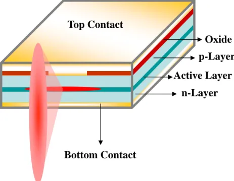
The first semiconductor laser was demonstrated with a p-n junction by Nathan et al at IBM in 1962 [NDB+62]. However, a simple p-n junction laser is not efficient and a great improvement by using heterostructure was proposed by Kroemer [Kroe63]. The device structure of a typical hetero-structure laser diode is depicted in Fig. 1.4-1. The electrons in the valence band of active medium are electrically pumped to conduction band to achieve population inversion. The resonator cavity is formed by the cleaved facets which have a reflectivity of about 30% due to the large

discontinuity of refraction indices between semiconductor and air. The laser output is parallel to the epitaxial layers and emitting from the edge of the device. As a result such laser diodes are commonly referred as edge-emitting lasers (EELs).

There are many advantages of semiconductor laser over other types of lasers: They are compatible with modern electronics and are easy to use; the whole device is manufactured by traditional semiconductor process such that they are compact and low-cost; their lasing wave length can be engineered for special purposes. However, due to the extremely narrow emitting region, the beam profile of an EEL is elliptical with high divergence in one direction and is detrimental for coupling into optical fiber. Besides, EEL is typically under multi-mode operation because of the long cavity length and this would induce longitudinal mode hopping that is undesirable for application. These critical drawbacks motivated the invention of VCSEL.

The device structure of a modern VCSEL structure is schematically shown in Fig. 1.4-2 to make a comparison with an EEL. As indicated by its name, the directions of laser oscillation and output are perpendicular to the semiconductor wafer. The first VCSEL is invented by Iga and co-workers in 1979 [SIKS79], while only pulsed operation is permitted at cryogenic temperature. With usage of distributed Bragg reflector (DBR) as cavity mirror [OHKY83], room-temperature continuous wave (CW) lasing of VCSEL was achieved by the inventors in 1989 [KKI89]. On the other hand, the efficiency of VCSEL has a big breakthrough with the introduction of quantum wells as active medium [JHT+89]. The efficiency is also closely related to the lateral electric current confinement, which also guides the optical field. There are four types of electrical and optical confinement, air-post, ion-implanted, regrown, and oxide-confined structures, for the modern VCSEL devices [CC+97]. Among these, oxide-confined VCSEL has the highest efficiency and lowest threshold and the devices used in this work are of this type.

Resulted from the symmetric transverse optical confinement, VCSEL has good beam quality as was expected. The cavity length of VCSEL is consequently designed to be about one wavelength and permits single longitudinal mode lasing. Due to the thin active layer, VCSEL can be modulated with an ultra-high speed

[STB+93]. Since the reflected mirrors of VCSELs are fabricated during epitaxial growth, batch processing and on-wafer testing make VCSEL more cost-efficient. Meanwhile, VCSELs can be arranged to high-fill-factor 2D laser arrays [GMJ+99] and can be monolithically integrated with photodetector [HTW+91], waveguide [LLP+05], modulator [GGK+96], and mirror [KDR+08], etc. Owing to these advantages, VCSEL has been widely used in optical communication [EFM+96, GAL98].

Despite that VCSEL is superior to EEL in many aspects VCSEL still has two shortcomings that do not exist in EEL. First, the output power of VCSEL is limited by the thin active medium. In contrast, high output power can be achieved by enhancing the length of the laser diode. Though high output power of VCSEL can be realized by enlarging the aperture, this will simultaneously result in high divergence angle since the Fresnel number of a cavity is proportional to the transverse area. Second, the polarization of EEL is fixed due to the extremely asymmetric emission region; while the polarization of VCSEL is unstable because its transverse aperture is isotropic. There is much effort to deal with these two problems: High-power fundamental-mode operation of broad-area VCSEL can be attained by manufacturing a photonic crystal on the surface [KSL+08] and integrating with monolithic micromirror [KDR+08]; the polarization of VCSEL can be controlled by several way [BCSR99, VdS+06]. However, our goal here is not to overcome the two problems but base on the two characteristics to explore interesting pattern formations in VCSELs.

Pattern formation [Lam98, CH99] is the spontaneous development of spatial (-temporal) nonuniformities of non-equilibrium systems under homogeneous external condition and has attracted much interest in chemistry [POS97], biology [LLM06], and physics [GL99]. Recently, Hegarty et al. have reported interesting pattern formations in the transverse mode of large-aperture oxide-confined VCSELs [HHMC99, HHP+99]. Besides, optical vortices have also been shown to spontaneously form in implanted VCSEL [SO99]. More recently, broad-area VCSELs have been shown to maintain cavity solitons [BTB+02, TAFJ08]. Most

importantly, it has also shown that the near-field transverse patterns of broad-area oxide-confined VCSEL are analogous to the mesoscopic wave functions of quantum billiards [HCLL02, CHLL03a, CLS+07, CSCH08]. The main idea of this dissertation is based on this interesting analogy.

As mentioned above, the polarization of VCSEL is unstable due to the isotropic gain region and birefringence. Generally, VCSEL emits linearly polarized light field in one direction at near-threshold current. As the injection current increases, the polarization behaviors of VCSEL becomes more complicated. One general condition is that two orthogonal linear polarization states independently coexist. Another interesting phenomenon is the polarization switching, in the process the lasing polarization state switches to the perpendicular one [AS01, MFM95, vEWW98]. Here a third case in which the transverse pattern has different morphology at different polarization angles is concerned [Erdo92, PTMA97]. In fact, this condition corresponds to the formation of vector field [CHLL03b], which also has been studied in various laser systems [Gil93, VKMR01, CLH06, LCH07]. Final part of this dissertation is to analyze the vector singularities embedded in the vector field emitted from VCSEL.

Top Contact

p-Layer

Oxide

Active Layer

n-Layer

Bottom Contact

Fig. 1.4-1. Schematic diagram of an edge-emitting laser. The laser output is parallel to the semiconductor layers. The out put beam is highly diverged due to the thin emission region.

Microsoft Office PowerPoint 2003.lnk

Fig. 1.4-2. Schematic diagram of a VCSEL. The laser output is perpendicular to the wafer. The isotropic aperture results in a good beam quality.

Oxide Layer

Active Layer

n-type DBR

Top Contact

p-type DBR

Bottom Contact

Submount

n-substrate

1.5 Overview of Thesis

The main text of this dissertation is structured as follow:

In chapter2 quantum billiards is employed to explore the classical-quantum correspondence of regular and chaotic systems. In Sec. 2.1 the classical POs and quantum eigenstates of square are reviewed and then the coherent states with wave functions localized on classical POs will be introduced. Similar process is done for an equilateral-triangular billiard in Sec. 2.2. In the final section of chapter2, the stadium billiard is used to demonstrate the quantum properties of chaotic systems. In chapter3 the analogous observations on various quantum-billiard wave functions from transverse modes VCSELs are presented. The first section of this chapter justifies the analogy between the transverse mode of VCSELs and the wave functions of quantum billiards. After which the experimental setup will be shown. The typical lasing modes of the square billiard are presented in Sec. 3.3. What follows is the chaotic modes generated by a rippled-square VCSEL. Finally, equilateral-triangular shaped VCSEL are shown to exhibit mixed properties of regular and chaotic system.

In chapter4, we investigate the time evolutions, probability currents, and OAM densities of eigenstate, coherent state, and chaotic state released of 2D square billiard. The time evolution of a stationary wave function abruptly released from 1-D infinite potential is first reviewed in the opening section. In Sec. 4.2, we extend to study the transient dynamics of various wave functions with a suddenly removal of 2-D square billiards. In third section of chapter4, we utilize the similarity between paraxial optics and 2-D non-relativistic quantum mechanics to analogously observe the time evolutions of coherent waves released from quantum billiards by free-space propagation of transverse modes of VCSELs. In final part of chapter4 we are to analyze the linear and angular momentum densities of the light beam emitted from VCSELs by analogously calculating the probability current and angular momentum

densities of coherent waves released from quantum billiard.

From chapter1 to chapter4, the observed patterns are all lasing in unipolarization and have their phasor amplitudes to be scalar field. In chapter5, we will consider the vector field formation in the transverse modes of VCSELs. In first section of chapter5 we present a polarization-entangled pattern associated with two superscars modes in a square shaped VCSEL. We reconstruct the patterns in two orthogonal polarization states by SU(2) coherent states to manifest the vector field and vector singularities. Similar experimental method as that in Sec. 5.1 is applied to originally generate a chaotic vector in Sec. 5.2. By using the eigenfunction expansion technique, the vector field is reconstructed to unambiguously analyze the vector singularities embedded in a chaotic vector field.

Chapter 2

Wave Functions of

Quantum Billiards

As revealed in Sec. 1.1, the eigenenergy of a regular quantum system can be determined by the old quantum theory with the help of the classical POs. On the other hand, the behavior of the quantum particle was not understood until Schrodinger particle was not understood until Schrodinger put developed the wave mechanics and Born interpreted the wave function by probability density. With Schrodinger equation, the wave function of integrable system can be analytically solved. In contrary, the wave function of chaotic system is still mysterious until Berry conjectured that chaotic wave function should be Gaussian random wave [Berr77]. With numerical calculation, the morphology of chaotic wave function was visualized [MK79, MK88]. More importantly, Heller showed that in addition to random phase filed some eigenstates of chaotic system will localize on the unstable PO [Hell84]s. Such kind of wave functions were called scar [Hell84]. For a chaotic system, both types of high-order wave functions, random wave or scar exhibit classical behaviors, as indicated by Bohr’s correspondence principle. Nevertheless, the highly-excited eigenstate of regular system do not reveal classical properties even with quantum number approaching to infinity.

In this chapter quantum billiards, which is one of the standard models (the other two are harmonic oscillator and Hydrogen atom) for studying quantum physics, is employed to explore the classical-quantum correspondence of regular and chaotic systems. In first section the classical POs and quantum eigenstates of square are reviewed and then the wave functions of superscar will be introduced. In Sec. 2.2 similar process is done for an equilateral-triangular billiard. Finally, the stadium billiard is used to demonstrate the quantum properties of chaotic systems.

The square billiard is one of the simplest billiards that is completely integrable in classical mechanics [Wier01, dSF01]. In a square billiard each family of periodic orbits can be denoted by three parameters ( , , )p q , where p and q are two positive integers describing the number of collisions with horizontal and vertical walls, and the parameter  (    

/ )

) that is related to the wall positions of specular reflection points [BB97, vonO94, Robi97]. Some examples of orbit families are shown in Fig. 2.1-1. It can be seen that the trajectory constitute a single, nonrepeated orbit provided that p and q are relatively prime. On the other hand, if p and q have a common factor f, the orbit family can be recast as the primitive periodic orbit

( / , / ,p f q f  f and f is the number of repetitions of the primitive periodic orbit. Since the square billiard is separable, the quantum eigenstates of square billiard are just the multiplication of the eigenstates of 1-D infinite potential well with variables in x and y 1 2 1 2 , 2 ( , ) sin( ) sin( ) n n n x n y x y a a a     (2.1.1)

Fig. 2.1-2 displays some of the eigenstates with their quantum numbers labeled below the figures. We can see that conventional eigenstates of a square billiard do not manifest the properties of classical periodic orbits even in the correspondence limit of large quantum numbers.

To construct the wave functions associated with periodic orbits, the SU(2) coherent state are extended to the square billiard [CHL02, CHLL03a]

1 , , , , ( 1 ) 0 1 0 1 ( , ) ( , ) 2 2 ( ) ( ( 1 sin[ ]sin[ ] 2 M p q M iK N M _M K qN pK pN q M K K M M iK K M K x y C e x y qN pK x pN q M K y C e a a a     )                 





(2.1.2) In order to understand the properties of the stationary coherent, we rewrite it as

1 [ ] ( 1) [ ( )] , , , 0 1 [ ] ( 1) [ ( 0 1 ( , ) 2 + p q M i qN x pN y iq M y iK x y p q _{a a a a a} N M K p q M i qN x pN y iq M y iK x y a a a a a K x y e e e a M e e e      _       _                    _ 





)] 1 [ ] ( 1) [ ( 0 1 [ ] ( 1) [ ( 0 ( , ) 1 { ( , ; 2 p q M i qN x pN y iq M y iK x y a a a a a K p q M i qN x pN y iq M y iK x y a a a a a K i x y e e e e e e e F x y a M      _      _                      _   





( , ) ( , ) ( , ) ) ( , ; ) ( , ; ) ( , ; )} i x y i x y i x y e F x y e G x y e G x y                   )] )] (2.1.3) , where 1 [ ( )] 0 ( , ; ) p q M _{iK x y} a a K F x y e   _        



, 1 [ ( )] 0 ( , ; ) p q M _{iK x y} a a K G x y e   _        



, and ( , )x y [qN x pN y] q M( 1) a a a y    

     . Since the property of the

functions ( , ; )F x y_  and G x y_( , ; ) is similar to the Dirichelet kernel, the stationary coherent state has maximum value whenever

2 p q x y a a   n      (2.1.4)

, which coincide with the classical trajectories of periodic orbits labeled as ( , , )p q . Fig. 2.1-3 displays the stationary coherent states _50,20p q, ,( , )x y associated with the periodic orbits shown in Fig. 2.1-1. It can be seen that the wave functions of

, , , ( , )

p q N M x y



 well localize on the periodic orbits ( , , )p q  . Furthermore, the

velocity of classical particle is at minimum at the specular reflection points and therefore |_{N M}p q, ,_, ( ,x y) |2 becomes extremely large at these points.

The wave given in (2.1.2) represents a traveling-wave property. The

standing-wave representation can be obtained by using , , * , ,

, ( , ) , ( , )

p q p q

N M x y N M x

 

   y . Including the normalization constant, the standing-wave forms can be expressed as

1 , , , ₁ 0 ( , ) M K C  x y 0 2 2 / ( ) cos( ) sin[ ] cos ( ) M p q M N M K K M K a qN pK x C K a C K     



  



 ( ( 1 ) sin[ pN q M K y] a      (2.1.5) and 1 , , , ₁ 0 ( , ) M K S  x y 0 2 2 / ( ) sin( ) sin[ ] sin ( ) M p q M N M K K M K a qN pK x C K a C K     



  



 ( ( 1 ) sin[ pN q M K y] a      (2.1.6).

Here we only show the wave pattern because the wave pattern

generally has the same properties. The N dependence of the wave

pattern is presented in Fig. 2.1-4. We can see that large value of N

naturally results in high mode order, since stands for the central quantum

number in the expansion. The M dependence of the wave pattern is

presented in Fig. 2.1-5. It can be seen that the larger the value of M is, the more strongly the wave pattern localize. This fact can be understood from the expressions of , , 2 , |C_{N M}p q( , )x y (qN pN, ) | | , , , |S_{N M}p q(x ( , F x 2 , ) |y , , 2 , |C_{N M}p q( , ) |x y ; ) y , , 2 , |C_{N M}p q( , )x y ( G x, ; )y 

 and  , which are similar to Dirichlet kernel having narrower

(p,q)

ψ

(1,1)

(2,1)

(3,2)

Fig.2.1-1. Some classical periodic orbits denoted by ( , , )p q  , where p and q are two positive integers describing the number of collisions with horizontal and vertical walls, and the parameter  (   ) that is related to the wall    positions of specular reflection points.

3  2 3  0 ₂  (p,q) ψ (1,1) (2,1) (3,2)  3  2 3   0 ₂

Fig.2.1-2. First some eigenstates and the one of ( ,n n_{1 2})(30,30). We can expect that conventional eigenstates do not manifest the properties of classical periodic orbits even in the correspondence limit of large quantum numbers.

(1,1)

(2,1)

(2,2)

(3,1)

(1,3)

(3,2)

(2,3)

(4,1)

(1,4)

(3,3)

(1,2)

(30,30)

(1,1)

(2,1)

(2,2)

(3,1)

(1,3)

(3,2)

(2,3)

(4,1)

(1,4)

(3,3)

(1,2)

(30,30)

(p,q)

ψ

(1,1)

(2,1)

(3,2)

Fig.2.1-3. Stationary coherent states _50,20p q, ,( , )x y associated with classical periodic orbits ( , , )p q . 3  2 3  0 ₂   (p,q) ψ (1,1) (2,1) (3,2) 3  2 3  0 ₂   (p,q) ψ (1,1) (2,1) (3,2)  3  2 3   0 ₂

Fig.2.1-4. The N dependence of the wave pattern |C1,1,0.6_N,5 ( , ) |x y 2. It can be seen that N is related to the mode order.

1,1,0.6 2

|

C



( , ) |

x y

1,1,0.6 2 40,5

|

C



( , ) |

x y

1,1,0.6 2 20,5

|

C



( , ) |

x y

30,5

Fig.2.1-5. The M dependence of the wave patterns |C1,1,0.6_30,M( , ) |x y 2. It can be seen that M is related to the localization of the patterns.

1,1,0.6 2 30,5

|

C



( , ) |

x y

1,1,0.6 2 1,1,0.6 2 30,20

|

C



( , ) |

x y

30,15

|

C

( , )

x y |

2.2 The Equilateral-Triangular Billiard

The equilateral-triangular billiard is a classically integrable but non-separable system. Let three vertices of an equilateral-triangular billiard to be set at (0, 0), ( / 2, 3 / 2)a a , and (a/ 2, 3 / 2a ) . The formation of classical periodic orbits can

be also denoted by three parameter ( , , )p q  , where the parameter p and q are

nonnegative integers with the restriction that p ; the parameter q  is in the range of 0 to  . The sign of  and the parameter p and q correspond to the initial angle of the billiard ball by [DB02, CH03]

1 tan( ) sgn( ) 3 p q p q      (2.2,1)

, where the initial angle  is with respect to horizontal. Assuming the initial position to be on y axis, the parameter  can be related to the initial position by

0 1 3 | 2 a y p q |     . (2.2.2) Some sample orbit families are given in Fig. 2.2-1. In terms of p and q, the path length can be written as

2 2

, 3

p q

L  a p q  pq, (2.2.3) except for the isolated orbits such as (1,1, ) [DB02].

The eigenstates in an equilateral triangular quantum billiard have been derived by several groups [Shaw74, RB81, LB85]. The wave function for the two degenerate stationary states can be expressed as