在嵌入式爪哇虛擬機器中設計並實做動態電壓頻率調整技術

國

立

交

通

大

學

資訊工程學系

碩

士

論

文

在嵌入式爪哇虛擬機器中設計並實作

動態電壓頻率調整技術

Design and Implementation of Dynamic Voltage and Frequency

Scaling for Embedded Java Virtual Machine

研 究 生：陳裕生

指導教授：單智君 博士

在嵌入式爪哇虛擬機器中設計並實作

動態電壓頻率調整技術

Design and Implementation of Dynamic Voltage and Frequency Scaling for

Embedded Java Virtual Machine

研 究 生：陳裕生 Student：Yu-Sheng Chen

指導教授：單智君 博士 Advisor：Dr. Jean Jyh-Jiun Shann

國 立 交 通 大 學

資 訊 工 程 學 系

碩 士 論 文

A Thesis

Submitted to Department of

Computer Science and Information Engineering College of Electrical Engineering and Computer Science

National Chiao Tung University in Partial Fulfillment of the Requirements

for the Degree of Master

In

Computer Science and Information Engineering August 2005

Hsinchu, Taiwan, Republic of China

在嵌入式爪哇虛擬機器中設計並實作

動態電壓頻率調整技術

學生：陳裕生

指導教授

：

單智君 博士

國立交通大學資訊工程學系碩士班

摘要

在執行程式過程中動態改變處理器的電壓以及執行頻率（Dynamic Voltage and Frequency Scaling, DVFS）可顯著的降低電耗。因為 JAVA 在嵌入式系統上受到重視， 所以本論文在嵌入式 JAVA 虛擬機器上發展了一套完整的 DVFS 實作。我們修改現有的 DVFS 策略，其主要參考目前工作的程式中記憶體存取時間以及處理器計算時間的比例， 計算適合的電壓，節省電耗。修改並發展出一套完整的方法論，在不同的平台下都可以 用類似的方式來估算記憶體存取時間以及處理器計算時間的比例，其誤差在本論文的實 驗環境下小於 8%。實做之 DVFS 系統包含兩種運作方式，其中以時間間隔為基礎的方式 可以在效能損失 15.89%~ 41.16%的情況下，達到 12.04%~28.68% 的電耗節省。 我們同 時驗證，以函式方法為基礎的系統並不適合使用於嵌入式爪哇虛擬機器中。

Design and Implementation of

Dynamic Voltage and Frequency Scaling for

Embedded Java Virtual Machine

Student : Yu-Sheng Chen Advisors : Dr. Jean, J.J. Shann

Department of Computer Science and Information Engineering National Chiao Tung University

ABSTRACT

Dynamic voltage and frequency Scaling (DVFS) is recognized as one of the most effective power reduction techniques. JAVA is getting popular in mobile embedded systems in recent year. Thus we propose a low-power research platform on an embedded JVM and implement DVFS on it. We refer to an accurate DVFS algorithm which calculates proper frequency of a program according to the ratio of on-chip computation time to off-chip access time. Proposed methodology for estimating the ratio of on-chip computation time to off-chip access time can be applied on defacement platforms. On our experiment platform, average error of estimations is less than 8%. Implemented design contains two schemes. Proposed interval-based design reduces 12.04%~28.68% energy consumption of the CPU with 15.89%~ 41.16% performance losses. We also experiment the potential of method-based design. And we conclude that method-based design is not suitable for embedded JVMs.

誌謝

本篇碩士論文得以順利完成，必須歸功於來自各方的指導、幫助以及鼓勵。其中， 指導教授單智君老師仔細而有耐心的教導，是我得以完成畢業口試及論文的主要原因， 在此獻上誠摯的感謝。 在此也必須要感謝驗室的另一位大家長、同時也是口試委員的鍾崇斌教授，和口試 委員盧能彬博士，由於他們的指教與建議，這篇論文才得以更加完整與確實。 在此也要感謝同實驗室的學長、同學們。彥銘、治瑋、敬中，我不會忘懷大家共同 度過的那許多無眠的夜晚，不論是精神上的互相激勵與安慰，或是學業研究上的討論指 導，都是因為有你們，才有辦法順順利利度過這兩年並得以完成學業。俊諭、欽毓、彥 志，沒有你們，就沒有我現在對於 JAVA 的認識與了解。耀中，你讓我了解什麼叫做研 究的態度與精神。綜禧，每逢星期一就會特別想念你，而且實驗室也因為有你，而顯得 歡樂許多。 最後，感謝與我關係最密切的家人們。父親、母親，沒有你們，就沒有現在的我， 我可以無後顧之憂的投入課業及論文研究中，都是因為有你們無條件的支持。俊丞，謝 謝你適時的關懷與激勵，以及那些貼心的禮物。惠瑜，如果沒有你，我無法想像研究生 的生涯該如何度過，謝謝你，在這一年多以來對我付出的關懷與照顧，這本論文，也是 因為有你而得以順利產生完成的。 謝謝，沒有你們，就沒有這篇論文。 陳裕生 2005. 9. 7

Contents

摘要

... i

ABSTRACT ...ii

誌謝

...iii

List of Figures ... vi

List of Tables...vii

Chapter 1

Introduction ... 1

1.1 Power Consumption of the Embedded Applications...1

1.2 Dynamic Voltage and Frequency Scaling (DVFS) ...1

1.3 Popularity of Embedded Java Virtual Machine...2

1.4 Research Motivation and Objectives...2

1.5 Organization of This Thesis ...3

Chapter 2

Background... 4

2.1 Java Technology...4

2.1.1. JVM Benefits...5

2.2 Dynamic Voltage and Frequency Scaling ...6

2.2.1 Generic Flow of DVFS...8

2.2.2 Implementation Levels of DVFS...9

2.2.3 Granularity Levels of DVFS ...11

2.3 Related Works ...13

2.3.1 Process Cruise Control ...13

2.3.2 Virtual-Machine Driven Dynamic Voltage Scaling ...15

2.3.3 DVFS based on the Ratio of Off-chip to On-chip Times...17

Chapter 3

System Design ... 20

3.1 System Overview...20

3.2 System Flow and Dynamic Profiler ...22

3.2.1 Working Flow of Interval-based Scheme...22

3.2.2 Working Flow of Method-based Scheme...23

3.3.1 Selection of Input Hardware Events...25

3.3.2 Linear Regression Model ...27

3.4 DVFS Mechanism ...28

Chapter 4

Experiments ... 29

4.1 Methodology...29 4.2 Experiment Environment...29 4.3 Benchmarks ...32 4.4 Experiment Results...32

4.4.1 Efficiency of Interval-based DVFS Scheme ...33

4.4.2 Efficiency of Method-based DVFS Scheme ...35

4.4.3 Comparison of Interval-based and Method-based Scheme ...36

Chapter 5

Conclusion and Future Work... 39

5.1 Conclusion...39

5.2 Future Work...41

List of Figures

Figure 2-1 : Example of Energy-Saving in DVFS ...7

Figure 2-2 : Generic Working Flow of DVFS...8

Figure 2-3 : Implementation Levels of DVFS...9

Figure 2-4 : Interval Level DVFS ...11

Figure 2-5 : Intertask Level DVFS...11

Figure 2-6 : Intratask Level DVFS...12

Figure 2-7 : Frequency Domain...14

Figure 2-8 : Estimated Total Run Time...16

Figure 3-1 : System Architecture ...21

Figure 3-2 : Working Flow of Interval-based Scheme ...23

Figure 3-3 : Working Flow of Method-based Scheme ...24

Figure 4-1 : Actual Performance of Interval-based Scheme ...33

Figure 4-2 : Energy Consumption of Interval-based Scheme ...34

Figure 4-3 : Actual Performance of Four benchmarks under Method-based Scheme ...35

Figure 4-4 : Energy Consumption of Four benchmarks under Method-based Scheme ...36

Figure 4-5 : Actual Performance of Interval-based and Method-based Schemes ...37

List of Tables

Table 2-1 : Comparison of Related Works...19

Table 3-1 : Event Category of PXA27x ...26

Table 3-2 : Correlation of HW events to CPI...27

Table 3-3 : Frequency Mapping Table ...28

Table 4-1 : Features of Intel PXA27X Developer’s Kit...30

Table 4-2 : V/F Switching Abilities of PXA27x ...30

Table 4-3 : Mapping Table of Frequency and Voltage ...31

Table 4-4 : Mapping Table of Frequency and Voltage for Turbo-mode...31

Table 4-5 : Descriptions of Benchmarks ...32

Table 4-6 : Experiment Results of Best Settings...38

Chapter 1 Introduction

In this chapter, we will present some introduction materials to help readers to get better understand of basic concepts behind our research. First, we remind that the importance of reducing power consumption of embedded applications. Second, we simply introduce and discuss the dynamic voltage and frequency scaling. Third, we explain why embedded JAVA environment becomes popular in recent year. After the introduction come our research motivation and objectives. In the final, we provide the organization of this thesis.

1.1 Power Consumption of the Embedded Applications

The increase in user demands for mobile and embedded systems requires an equivalent increase in processor performance, which causes an increase of the power consumption of these devices. Managing energy consumption, especially in devices that are battery operated, increases the number of applications that can run on the device and extends the device’s battery lifetime. With efficient power management, an increase in mission duration and a decrease in both device weight and total cost of manufacturing and operation can be achieved [1].

1.2 Dynamic Voltage and Frequency Scaling (DVFS)

Dynamic voltage and frequency Scaling (DVFS) is recognized as one of the most effective power/energy reduction techniques. In a DVS equipped processor, such as Intel's XScale processors, the CPU voltage and frequency can be changed on-the-fly [2]. The key to

make use of this technique is to reduce clock frequency (and of course, reduce it with voltage) of processor only when it is not critical to meet the deadlines of software or CPU is stalled by memory or I/O systems [3]. Since the performance of those memory-bound applications is limited by memory, reducing of processor frequency will not cause significant performance degradation but yielding significant reduction of energy consumption [4].

1.3 Popularity of Embedded Java Virtual Machine

JAVA is getting popular in mobile embedded systems in recent year because of four reasons discussed later [5]. Portability, platform neutrality, means that programmer can write code once and runs everywhere without taking care about underlay system architectures. Dynamic nature means that the code can be used as data, download or upgrade on demand, thus it reduce the cost of redistribution. Most importantly of all, the security mechanism of JAVA provides trust and reliable environment of embedded environments and since many of them must work for a long term without restarting or upgrade. Finally, the small footprint of JAVA bytecode and runtime memory requirement decreases the cost of embedded applications.

1.4 Research Motivation and Objectives

Since the need of reducing power consumption of embedded JAVA environments is increasing, we propose a low-power research platform on a JAVA embedded system. Using this platform, we can easily collect information about a program in its running time. So we can apply some low-power techniques according to collected information to reduce power consumption. We focus on DVFS technology because of the effectiveness provided by it.

DVFS research in virtual machine (VM) proposed by Haldar et al. [6] is the first and the only one in the past. They declare that VM has some advantages of implementation of DVFS. First, virtual machines have an infrastructure allowing them to profile and reoptimize programs in execution. Second, VM can gather and make use of information from HW, OS, VM, and programs at run time to provide accurate prediction of future behavior of programs. However, there exist some disadvantages in Haldar et al.’s effort. First, they do not discuss the efficiency of dynamic profiler. Profiling overhead may increase run time and power consumption. Second, the frequency/voltage decision policy proposed by them is a simple and inaccurate heuristic and it may yields inaccurate prediction of needed frequency of programs.

Thus our objectives are as follows. Design and implement effective DVFS for embedded JAVA virtual machines which reduces power and energy consumption while meeting the performance requirements specified by user. We will focuses on designing a low run-time overhead dynamic profiler and implementing an accurate frequency/voltage decision policy

1.5 Organization of This Thesis

The remaining parts of this thesis are organized as follows. The next chapter provides more detailed background knowledge about DVFS and JAVA technique, and introduces some related works. Chapter 3 details on our design and implementation of DVFS in JVM. In Chapter 4, experiment results are exhibited. In the end we make a brief summary and conclusions in Chapter 5.

Chapter 2 Background

This chapter provides more background details on JAVA technology and DVFS. We will first introduce JAVA technology. Then, background of DVFS will be presented. We also discuss some related work which inspires our research.

2.1 Java Technology

Although generally used to refer to a computer language, Java is a rather a complete architecture in reality. It consists of four distinct but interrelated components [6].

• Java programming language • Java class file format

• Java Application Programming Interface (Java API) • Java Virtual Machine (JVM)

A Java program is written in Java programming language, and then compiled into Java class files by Java source compiler. Java class files can be executed on any environment that equips a JVM. Also, the Java program can access predefined libraries or system resources (such as I/O, for example) by calling methods in the classes that implement the Java API. During program execution, JVM loads and executes user-written class files as well as these system classes that Java API defines.

2.1.1. JVM Benefits

Java Virtual Machine is definitely the key component among the all. It is responsible for the well-known advantages that Java possesses over traditional native execution system. Those advantages include:

• Cross-Platform Portability

Each type of processor has its unique instruction set. For example, the instruction set of x86 is not compatible with that of MIPS. Moreover, each operating system (OS) has its own application interface or system calls to upper application programs. As a result, programs compiled to run on one platform (combination of processor and OS) cannot be executed on others without recompilation. Java overcomes this limitation by inserting JVM between the application programs and the real environment. If JVM has been ported to the environment, Java programs can be first compiled to Java bytecode in the form of class files and then be executed over the JVM without any porting efforts. This encourages software reuse and alleviates great pains from programmers.

• Security of the Execution Environment

One of Java’s original intentions is its integration into the network environment. In this environment, class files can be automatically downloaded from network and be locally executed. They might be malicious and might do dangerous operations to the local execution system. To deal with this important issue, Java build up its own security model - the sandbox. As a brief explanation, Java verifies every class file from untrusted resources. The verification process mainly involves two steps in JVM. First, class file verification checks the layout and the contents of the class file. Second, bytecode verification checks if the bytecode within a

method adheres to predefined rules. For example, one basic rule is that all goto and branch instructions refer to valid bytecode addresses.

• Small Size of the Compiled Code

Due to the rich semantics and the stack-based operations, Java bytecode, the instruction set of JVM, is more compact space-wise than a statically compiled program. In other words, Java has high code density. According to [8], the dynamic average instruction size is 1.8 bytes. Compared with typical RISC instruction requiring 4 bytes, this result is satisfactory. For a speed-limited network environment or a memory constrained embedded

2.2 Dynamic Voltage and Frequency Scaling

In this subsection, we will describe background knowledge of DVFS. The term, DVFS, means that scale frequency with scaling voltage. According to [2] and equation below, there is a proper/lowest voltage for each clock frequency to run stably. Thus we can provide enough/lowest voltage for processor to run stably on current frequency to save power. The frequency can be estimated by the following equation,

dd t g V V V f 2 ) ( − ∝ ₍₁₎

where f is the frequency of processor, Vdd the supply voltage, Vt the threshold voltage, and

Vg the voltage of the input gate. The dominant source of power dissipation in a digital CMOS

circuits is the dynamic power dissipation [2],

2 dd V f c P∝ ⋅ ⋅ (2)

power is linear in frequency and quadratic in voltage. But we know that energy consumption,

E=Pt, where t is execution time, which is an inverse proportion to frequency. Thus we can

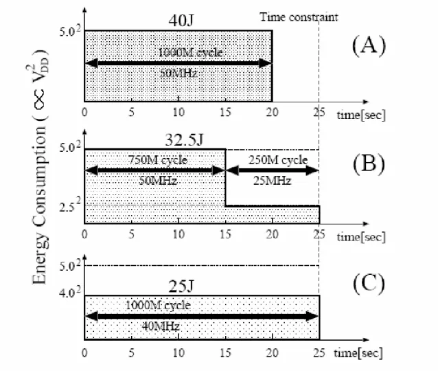
derive that energy is quadratic in voltage. There is trade-off between 1/frequency and voltage, between execution time and energy if we consider both performance and energy consumption. There are some clear examples in figure 2-1 [9].

Figure 2-1 :Example of Energy-Saving in DVFS

In figure 2-1 (A), program runs at highest frequency with highest voltage thus gets highest energy consumption even if the power supply is turned off after finishing the program. Under the given time constraint of 25 seconds, the voltage scheduling in (B) and (C) get better energy consumption.

2.2.1 Generic Flow of DVFS

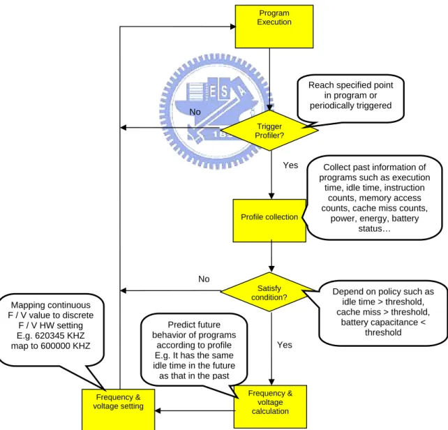
Figure 2-2 describes the generic flow of DVFS system. When running a program, DVFS system will trigger profiler at some time or at somewhere in code. After triggered profiler and collected needed information, the system needs to verify the condition of program of runtime and decide whether to scaling frequency and voltage or not. Collected information then will be analyzed by system to produce proper frequency and voltage for current status. After then, we need to map the continuous values to closet discrete hardware settings.

Program Execution Profile collection Frequency & voltage calculation Frequency & voltage setting Trigger Profiler? No Yes Satisfy condition? No Yes

Reach specified point in program or periodically triggered

Collect past information of programs such as execution

time, idle time, instruction counts, memory access counts, cache miss counts,

power, energy, battery status…

Depend on policy such as idle time > threshold, cache miss > threshold,

battery capacitance < threshold Predict future

behavior of programs according to profile E.g. It has the same idle time in the future

as that in the past Mapping continuous

F / V value to discrete F / V HW setting E.g. 620345 KHZ map to 600000 KHZ

2.2.2 Implementation Levels of DVFS

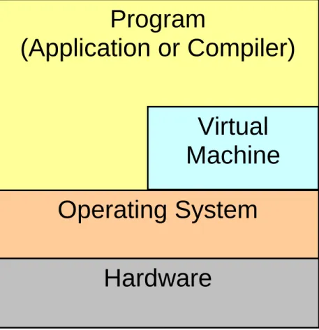
DVFS can be implemented in at a number of levels. These include the hardware level, operating system level, compiler level, virtual machine level, and application level. Nearly all DVFS research has focused on the first three levels. Though the hardware level provides mechanisms for reducing frequency and voltage, it also needs information about program behavior to decide when to apply these mechanisms. Techniques for deriving this information are too expensive to implement in bare hardware [10].

Operating System

Program

(Application or Compiler)

Hardware

Virtual

Machine

Operating systems have more information, namely, about what programs are running and what resources they use. Thus, they can make DVFS decisions based on CPU usage patterns. However, operating systems lack forward looking information about program behavior and are hence limited to extrapolating future behavior from past behavior [3][4][11].

Compilers, however, receive an entire program as input. Thus, they can predict with greater accuracy the paths a program’s execution will take. Compilers can make DVFS decisions at a finer granularity than operating systems by inserting DVFS instructions into program regions such as basic blocks. Nevertheless, statically optimizing compilers lack runtime information and often resort to exhaustive simulation or previously collected offline profiles to decide what program regions should slow down and how much they should slow down. Once made, these decisions remain fixed for a program’s execution [12].

Like compilers, virtual machines have a model of future program behavior and can thus make more accurate power management decisions than operating systems or bare hardware. However, unlike static compilers, virtual machines have an infrastructure allowing them to profile and reoptimize programs in execution. This dynamic optimization infrastructure allows virtual machines to continuously adapt power management decisions to varying execution behavior [6].

At the application level, programmers can make design decisions that reduce execution time and create opportunities for slowing down the processor. However, doing all of the analysis for DVFS at the application level may place too much of a burden on programmers [2].

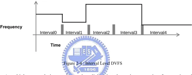
2.2.3 Granularity Levels of DVFS

DVFS has been explored at different granularity levels. These include the interval level, intertask level and intratask level. At the largest granularity are interval-based policies that regularly adjust processor speed based on prior workloads. The simplest algorithm of this kind is PAST [11]. PAST adjusts CPU speed at fixed length intervals based on the idle and active cycles of the previous interval. If the idle cycles exceed a threshold, it slows down the processor. Else if the active cycles are higher, it speeds it up.

Interval1 Interval2 Interval3

Interval0 Interval4

Time Frequency

Figure 2-4 : Interval Level DVFS

At a higher granularity are intertask policies that determine execution frequencies of individual tasks. The simplest example of an intertask policy is Energy-priority scheduling [13]. This policy maintains an even workload distribution as new tasks enter a system, to minimize battery drain rate. In every iteration, EPS schedules the task with furthest deadline and fewest overlapping tasks. It computes the minimum workload increase due to the new task and speeds up already scheduled tasks to make room and fill up slack.

Task1 Task2 Task4

Time Frequency

Task3 Task0

Intratask approaches vary clock frequency and voltage within individual tasks. These approaches have been implemented in operating systems and compilers. Example of OS-assisted intratask policies are Dudani et al. [14]. To combine EDF scheduling with frequency scaling, Dudani et al. split each task the scheduler chooses into two subtasks, later running at full speed and the earlier running slower. They choose the earlier subtask’s speed to keep the combined execution time of both subtasks below the average execution time for the whole task.

Compiler-assisted intratask DVFS by Hsu and Kremer [15] discusses how to select regions where DVFS decisions should be made. The idea is to instrument a program with profiling code and execute the program to build a table of execution frequencies and average cycles for each region under all possible clock frequencies. Using this exhaustive approach, Hsu and Kremer select the region whose slowdown minimizes energy dissipation and incurs the smallest increase in runtime.

Task0 Section Task0 Section Task0 Section Time Frequency Task0 Section Task0 Section Section : Program units, such as function, loop, basic block

2.3 Related Works

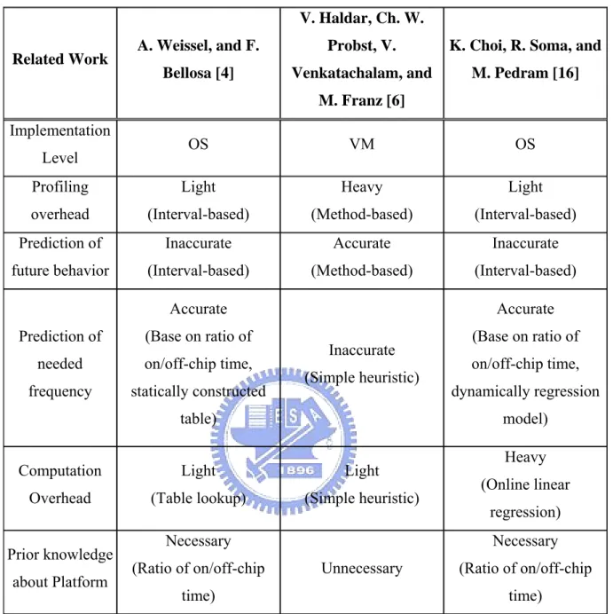
The first part of this subsection details on the related work which implements a DVFS algorithm in an operating system [4]. It gives a way to select suitable CPU frequency and voltage settings according to behavior of processes. This work inspires us to use hardware event counter to characterize program and choose proper setting of CPU. In the second subsection, we introduced a DVFS effort which is also implemented on JVM [6]. The final subsection introduces a novel and accurate DVFS algorithm implementing in an operating system [16]. This effort also makes use of hardware event counter to choose proper setting of CPU. It contains an online regression based algorithm which calculates frequency dynamically instead of looking up table. We implement a variation of this effort because of its accuracy.

2.3.1 Process Cruise Control

The subtitle of this effort is "Event-driven clock scaling". It suggests making use of some sort of event counts occurred at runtime to select a proper CPU frequency for a process. They use two hardware events as metric, memory requests and executed instruction counts. In fact, according to this related work, we can characterize program by analyzing hardware event counts and select proper frequency for each program.

They implement DVFS mechanism in an operating system. It samples hardware event counters for each process at each schedule point. At the same time, using past recorded hardware event counts to choose suitable execution frequency for selected process.

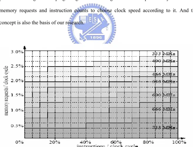
The proposed DVS strategy is based on statistics. They write special programs which can generate various hardware event counts, such as twenty memory requests and one thousand executed instructions. For each clock speed setting, they record execution time for each of these programs. The next step is to find the minimal clock speed which can be tolerated for given performance requirements. For experiment, they chose 10% as an acceptable performance loss. Using the minimal clock speed under different event counts, they construct a table named frequency domains (for an example see figure 2-7 [4]). An optimal clock speed is chosen by looking up this matrix.

As previously mentioned, the more memory accesses program does the less performance degradation program get when scaling down clock speed. They make use of memory requests and instruction counts to choose clock speed according to it. And this concept is also the basis of our research.

2.3.2 Virtual-Machine Driven Dynamic Voltage Scaling

To our knowledge, this is the first effort to implement DVS in JVM. Their system use recorded method execution time to predict expected execution time of a method. The expected execution time is then used to estimate clock speed of a method. The main concept of this research is to make use of trade-off between speed loss and energy saving. Main flow is described as follows.

1. Calculating new clock speed at the entry of a method. If it is changed (current clock speed doesn’t equal to maximum speed), it will not be scale to any new speed setting. 2.

3. Sampling the execution time of method after leaving it. Then calculating the average execution time and saving it.

The way to calculate suitable clock speed is trivial. This algorithm assumes that the application’s future execution time will be the same as the time it spent executing so far. The goal of equation (3) is to estimate total execution time when executing a specific method. In equation (4), the estimated time of method is in inverse proportion to clock. After adding overhead of switching, the total execution time after scaling is calculated. New clock speed is estimated by using equation (5).

Tapp Tmd Ttotal= +2× (3) Ts Tapp Fn Fm Tmd Tpre= × +2× +2× ₍₄₎ Ttotal Ka Tpre Ttotal< < × ₍₅₎

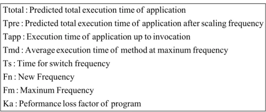
program of factor loss Peformance : Ka Frequency Maxinum : Fm Frequency New : Fn frequency switch for Time : Ts frequency maxinum at method of time execution Average : Tmd invocation to up n applicatio of time Execution : Tapp frequency scaling after n applicatio of time execution total Predicted : Tpre n applicatio of time execution total Predicted : Ttotal

Tapp

Tmd

Tapp

Tmd

Ttotal

Now

Figure 2-8 : Estimated Total Run Time

They made many correct design decisions, such as profiling each method [17], considering switching overhead, and making use of trade-off between speed loss and energy saving. But they don’t consider overhead of runtime profiling since this effort profiles at each method entry and exit. The simple heuristic they proposed has two problems. First, linear relation between run time and frequency yields inaccurate prediction of run time after scaling frequency. Second, over-predicted total run time of a application yields inaccurate prediction of frequency.

2.3.3 DVFS based on the Ratio of Off-chip to On-chip Times

The complete title of this related work is “Fined-Grained Dynamic Voltage and

Frequency Scaling for Precise Energy and Performance Trade-off based on the Ratio of Off-chip Access to On-chip Computation Times”. The key idea of this research is to make use

of runtime information about the external memory access statistics in order to perform CPU voltage and frequency scaling with the goal of minimizing the energy consumption while meeting the performance requirements. Unlike [4], it relies on dynamically-constructed regression models that allow the CPU to calculate the expected workload for the next time slot, and thus, adjust its voltage and frequency in order to save energy while meeting soft timing constraints. This is in turn achieved by estimating and exploiting the ratio of the total off-chip access time to the total on-chip computation time. The equations below show how to calculate the ratio of the off-chip CPI to on-chip CPI using regression model:

c MPI b

CPIavg = ⋅ avg + (6)

( } {

∑

∑

∑

∑

∑

+ − = + − = + − = + − = + − = − ⋅ ⋅ − ⋅ ⋅ = 1 2 , 1 2 , 1 , 1 , 1 , , ) ) ( ) ( ) ( ) ( N t t i i avg N t t i i avg N t t i i avg N t t i i avg N t t i i avg i avg MPI MPI N CPI MPI CPI MPI N b (7) N MPI b N CPI c N t t i i avg N t t i i avg

∑

∑

− + = + − = _{− ⋅} = 1 , 1 , (8) 1 , − = c CPIavgt t β ₍₉₎ )} ( { t t loss t f f PF f f max max 1 1 1+ ⋅ + ⋅ = + β (10)

In that DVFS system, CPI and MPI (memory request per cycle) are sampled each interval. The monitored event values are used to estimate coefficient b and c of regression equation (6), and then to use this equation to predict the ratio of off-chip CPI to on-chip CPI (equation (9)) of a program. Coefficients b and c at quantum t≥N , are calculated from the

last N event samples as equation (7) and (8). Once βt is obtained, the target CPU frequency for the next quantum, f t+1, is calculated from equation (10) with the specified PFloss factor.

Proposed DVFS algorithm has some advantages, such as light runtime overhead of dynamic profiler, accurate prediction of the program run time after scaling, and accurate prediction of needed frequency of program. In contrast, it has some disadvantages, such as inaccurate prediction of program behavior with interval basis, heavy runtime overhead of online regression calculation, and incompatible estimation of ratio on different platforms.

Finally, we present a comparison table of related works. We compare these three related works from different respects. This table contains implementation level, runtime profiling overhead, prediction accuracy of future behavior and needed frequency, runtime computation overhead and platform neutrality of them.

Table 2-1 : Comparison of Related Works

Related Work A. Weissel, and F. Bellosa [4]

V. Haldar, Ch. W. Probst, V. Venkatachalam, and

M. Franz [6]

K. Choi, R. Soma, and M. Pedram [16] Implementation Level OS VM OS Profiling overhead Light (Interval-based) Heavy (Method-based) Light (Interval-based) Prediction of future behavior Inaccurate (Interval-based) Accurate (Method-based) Inaccurate (Interval-based) Prediction of needed frequency Accurate (Base on ratio of on/off-chip time, statically constructed table) Inaccurate (Simple heuristic) Accurate (Base on ratio of on/off-chip time, dynamically regression model) Computation Overhead Light (Table lookup) Light (Simple heuristic) Heavy (Online linear regression) Prior knowledge about Platform Necessary (Ratio of on/off-chip time) Unnecessary Necessary (Ratio of on/off-chip time)

Chapter 3 System Design

This chapter details on design and software implementation. First subsection describes architecture of entire system and relations between all system components. In second subsection, we describe runtime profiling mechanism, DVS subsystem and working flow between them. Third section is the most important part of this research. It details on a modified DVS strategy from [16]. It uses hardware event counts to estimate future behavior (CPI) of a program.

3.1 System Overview

Our implementation is based on KVM (Kilobytes virtual machine) of version 1.04 [18]. As its name suggests, it is a special JVM for small embedded systems. The features of KVM are small code footprint, small memory footprint and simple architecture. Referring to [4], [6] and [12], we design and implement two kinds of schemes, interval-based and method-based. Our goal is to evaluate efficiency of interval-based scheme and to exploit the potential of method-based scheme. Figure 3-1 is the concept diagram of entire system. The rectangle in center is KVM. We add some software components to KVM that describe as follows.

•Dynamic Profiler:

This component takes reasonability for collecting runtime information of programs. Method-based profiler consists of two parts. First part collects invocation counts and durations of each method, then finds out those hot methods. Second part collects hardware event counts of each hot method. We record cycle, instruction, I/D cache miss, DTLB miss

counts. We also implement an interval-based profiler.

•DVS policy model:

According to the information provided by dynamic profiler, it estimates a suitable clock speed. We adapt policy/equation from [16] for our experiment platform. We will discuss this later.

•DVS mechanism:

According to the clock speed policy model estimated, it maps value to setting commands and sends them to processor to scale execution frequency. We use a customized Linux kernel module to implement this component.

When a program is being executed, the dynamic profiler is invocated in proper situation (periodically or at specified point). DVS policy model estimate proper clock speed according to profile collected. Then DVS mechanism is invoked.

Dynamic Profiler Processor DVFS Policy Model Cycles, Instructions, I/D cache misses, DTLB misses DVFS Mechanism KVM Interpreter Frequency & Voltage setting Method invocation counts Profiles Frequency & Voltage Original New Bytecode

3.2 System Flow and Dynamic Profiler

A complete DVS algorithm must consist two main important parts. First part is profiling behavior of programs. Second part is estimating clock speed according to profile. We present working flow of interval-based scheme firstly. Next, working flow of method-based scheme is proposed.

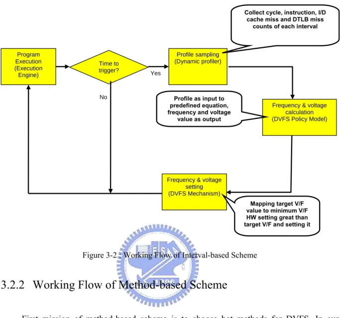
3.2.1 Working Flow of Interval-based Scheme

In a word, interval-based scheme samples hardware event counters at each interval. Length of interval is set to a multiple of V/F switching overhead to reduce the influence yielded by switching. Complete working flow is provided in Figure 3-2. At the beginning of each interval, DVFS system samples HW events, calculates frequency from events, maps frequency to actual HW setting and sets the setting.

Program Execution (Execution Engine) Profile sampling (Dynamic profiler)

Frequency & voltage calculation (DVFS Policy Model)

Frequency & voltage setting (DVFS Mechanism) Time to trigger? No Yes

Collect cycle, instruction, I/D cache miss and DTLB miss

counts of each interval

Profile as input to predefined equation, frequency and voltage

value as output

Mapping target V/F value to minimum V/F HW setting great than target V/F and setting it

Figure 3-2 : Working Flow of Interval-based Scheme

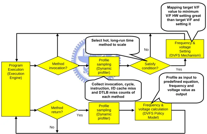
3.2.2 Working Flow of Method-based Scheme

First mission of method-based scheme is to choose hot methods for DVFS. In our design, hot methods are defined as frequent and long run-time methods. The goal of this limitation is to select suitable method with reducing the runtime overhead of profiling and calculation. In our design, profiling is done at each invoke bytecode to record duration and invocation counts. While a invoke bytecode is executed for some times, system will judge if it is suitable for DVFS by its average duration. Call site with short average durations will be replaced by a non-profiling bytecode to prevent continuing profiling at this call site.

After figuring out those hot methods, we use another profiler to record average hardware event counts of each of them. The collected hardware event counts include cycle,

instruction, I/D cache miss, DTLB miss counts. Those counts are collected by using a customized linux kernel module.

While the system collects enough information of the method and satisfies some assumption (cycle counts is bigger than a threshold), DVFS policy model will estimate a proper clock speed of it. If it decides to switch frequency, system will do change before executing the method. Figure 3-3 is the complete flow diagram of this section.

Program Execution (Execution Engine) Profile sampling (Dynamic profiler) Frequency & voltage calculation (DVFS Policy Model) Frequency & voltage Setting (DVFS Mechanism) Method invocation? Satisfy condition? No Yes

Collect invocation, cycle, instruction, I/D cache miss

and DTLB miss counts of each method Select hot, long-run time

method to scale Profile as input to predefined equation, frequency and voltage value as output Mapping target V/F value to minimum V/F HW setting great

than target V/F and setting it Profile sampling (Dynamic profiler) Method return? Yes No

3.3 DVFS Policy Model

This section describes the most important part of our effort, a modified DVFS algorithm from [16]. It is based on some import observation and assumptions. And the goal of it is to make use of slight speed loss to trade significant energy saving. As mentioned before, the speed of memory is much slower than processor so performance of program will be limited. Although we scale down clock speed of processor, it will not make significant degradation of performance [4]. In common, the scaling of processor will not degrade significant speed of memory access. So we assume the speed of memory will not be changed after changing the speed of processor.

Before explaining how to calculate proper frequency, we need to describe a methodology for selecting HW events to calculate ratio of on-chip CPI to off-chip CPI. Because the ratio is the most important variable in this policy and our target platform do not provide a trivial way to figure it out, we need to obtain the ratio by a more complicated way.

3.3.1 Selection of Input Hardware Events

Our target platform is Intel XScale PXA27x developer’s kit [19]. The processor in this platform contains four HW event counters and one cycle counter. We extend the policy from [16] by estimating the ratio of on-chip CPI to off-chip CPI with five counters. We extend the original regression model from two variables to four variables. Thus we need a methodology to select events with accurate prediction of CPIs. The complete flow is described as follows. We use our target platform as example to help understanding.

1. Select events belong to either on-chip or off-chip events except mixed. The intention of this step is to filter out unsuitable event. Since we want to calculate regression of off-chip and on-chip CPI, we filter out those mixed events. Table 3-1 provides examples for categorizing events on PXA27x. Except instruction executed event, we filter out all mixed events since we want to calculate CPIs.

Table 3-1 : Event Category of PXA27x

On-chip Off-chip Mixed

(5)Branch instruction executed (6)Misspredicted branch count (13)Number of times software changed the PC

(0)ICache miss count (3)ITLB miss count (4)DTLB miss count (8)Number of stall cycles due to

buffers full

(9)Number of times buffers are detected full

(11)DCache miss count (12)Number of write-back events

(1)Number of stall cycles for fetch unit

(2)Data dependency duration count (10)DCache access count (7)Number of instructions executed

2. Run benchmarks and collect all selected HW events at different frequencies. We using MiBench [20]and four programs from SPECJVM98 [21]. The real-life behaviors of programs on target platform are collected to help figure out the most important events since target platform provides limit number of counters.

3. Choose HW events with high correlation to CPI. Correlations of all events normalized with instructions counts to CPI are calculated for different frequencies. We choose three events of highest correlation to CPI, instruction cache miss, data cache miss, and data TLB miss counts. Table 3-2 present average correlations of events to CPI.

Table 3-2 : Correlation of HW events to CPI Event Correlation DTLB_MISS/INST(7) 0.5557 ICACHE_MISS/INST(1) 0.5287 DCACHE_MISS/INST(3) 0.5194 DCACE_WRITE_BACK/INST(13) 0.4263 DCACHE_FULL_STALL/INST(10) 0.3809 DCACHE_FULL_STALL_CONTIG/INST(11) 0.2948 ITLB_MISS/INST(6) 0.1804 BRANCH/INST(8) 0.0528 PC_CHANGED/INST(12) 0.0321 BRANCH_MISS/INST(9) -0.0624

4. Calculate linear regression coefficients of selected events to validate the accuracy. The error of selected events on PXA27x with those benchmarks is 8%

3.3.2 Linear Regression Model

Dynamic profiler samples CPI, instruction cache miss per instruction, data cache miss per instruction, and data TLB miss per instruction each time it is invoked. Sampled data are then fed to regression model (Equation 11) to calculate coefficients of Equation 12. The ratio of on-chip CPI to off-chip CPI (Equation 13) is calculated immediately. While β is calculated, proper frequency of next interval/method can be estimated by Equation (14).

CPIs Events Events Events Coffs=( T ⋅ )−1⋅ T⋅ (11) d DTMPI c DMPI b IMPI a CPI = ⋅ + ⋅ + ⋅ + (12) d DTMPI c DMPI b IMPI a⋅ + ⋅ + ⋅ = β ₍₁₃₎ 1 ) 1 ( max + + ⋅ ≥ β loss new PF F F ₍₁₄₎

factor loss Perfomance : PF Frequency CPU New : F frequency CPU Maxinum : F CPI to CPI of Raio : β CPI of samples K matrix, Kx1 : CPIs events HW 4 of samples K matrix, 4 K : Events d c, b, a, represent matrix, 4x1 : Coffs n instructio per miss TLB Data : DTMPI n instructio per miss Dcache : DMPI n instructio per miss Icache : IMPI n instructio per Cycles : CPI loss new max onchip offchip ×

There is a problem in implementation of online regression calculation. The runtime overhead of matrix operations is significant on target platform since it does not have float point processor and divider. It yields about 200k cycles on PXA27x platform to calculate a set of coefficients. So we also propose a static method using training sets to calculate coefficient offline. We will evaluate on/off line method in next chapter.

3.4 DVFS Mechanism

In order to obey performance requirement and simplify design, we use a conservative method for mapping calculated frequency into actual HW setting. It maps frequency produced by the policy model to minimum CPU frequency setting which is equal to or great than target frequency. Table 3-3 shows the example on our target platform.

Table 3-3 : Frequency Mapping Table Calculated

Frequency 624 ≤ f < 520 520 ≤ f < 416 416 ≤ f < 312 312 ≤ f < 208 208 ≤ f Mapped

Chapter 4 Experiments

This chapter is devoted to experiments. We first describe experiment methodology. Next, our hardware and software environment for experiments are detailed. Third, appropriate benchmarks are chosen for performance and energy evaluation. Finally, experiment results including speed performance and energy reduction are exhibited.

4.1 Methodology

In a word, evaluation of our design is done with two kinds of ways, measuring of real run time and simulating of relative energy consumption. Relative performance of speed is measured by performance monitor counters while running benchmarks and calculated with comparing to baseline KVM. Relative energy consumption is calculated with equation (15). All durations under different frequency settings in a run are record. According to F/V table (see Table 4-3 and Table 4-4), related energy consumption of this run can be calculated.

t V f

E∝ ⋅ _dd2⋅ ₍₁₅₎

4.2 Experiment Environment

Our effort is designed and implemented based on version 1.1 of Sun’s KVM [18], the reference implementation of J2ME CLDC. For our research usage, the KVM is ported to the Intel XScale PXA27x developer’s kit [19], an evaluation board which consist a PXA270 processor, 64MB SDRAM, LCD, and many other peripherals (see Table 4-1). This evaluation

board supports three kinds of mechanisms for switching frequencies and voltages of the processor (see Table 4-2). We use different mechanisms for different granularity of settings of our design.

Table 4-1 : Features of Intel PXA27X Developer’s Kit Feature Description

Processor Single issue super-pipelined(7~8) microprocessor

On-chip Memories

256 KB scratch-pad memory

32 KB, 32 ways set associative I/D cache 2 ways set associative mini D cache 2 KB, 2 ways set associative BTB 32 entry full associative I/D TLB

Off-chip Memories 64 MB SDRAM

32 MB Flash RAM Performance

Monitor 1 cycle counter, 4 event counters (support 14 events)

Limitation of V/F 13 MHZ ~ 624 MHZ, 0.9V ~ 1.5V Other peripherals LCD, USB, Ethernet, Serial ports…

Table 4-2 : V/F Switching Abilities of PXA27x

Description V/F coupling F only Turbo-mode (F only)

Delay ~1000 μs ~150 μs ~5 μs # of settings (according to bus frequency) 1~7 1~7 1~3 Granularity of Our Design > 10 ms > 1ms > 500μs

We also add supporting code of performance monitoring and V/F switching for PXA270 processor to linux kernel version 2.4.21. Setting using in experiments of our design is detailed as follows. For SPECJVM98, heap memory size is set to 8MB. With exhaustive experiment, we set length of sample queue of regression model to 10.

Interval-based scheme is experimented with 1000, 100, and 10 ms interval. Because average run time of benchmarks is less than ten seconds, interval longer than 1000 ms is unreasonable. The timer mechanism support by OS/HW put the limit of shortest length of the interval.

Method-based scheme is experimented with hotspot thresholds of 5 invocation counts and 500 us length. Currently, it is the best setting of method-based scheme with considering performance of speed and energy and runtime overhead of profiling and switching. In final, relations between frequency and voltage settings using in experiments are presented in Table 4-3 and Table 4-4.

Table 4-3 : Mapping Table of Frequency and Voltage

Frequency (MHZ) 208 312 416 520 624

Voltage (mv) 1150 1250 1350 1450 1500

Table 4-4 : Mapping Table of Frequency and Voltage for Turbo-mode

Frequency (MHZ) 208 312 624

4.3 Benchmarks

Due to the limited APIs that J2ME CLDC specifies, common Java benchmarks can not be applied in our experiment. By referring to related academic researches, we find that there are rare J2ME benchmarks suited for our experiments. Thus we modify KVM and four benchmarks from SPECJVM98 [21]. SPECJVM98 is commonly used in academic researches for JVMs for desktops or servers. But four benchmarks of it can be modified to run on embedded JVM with reasonable resource. Below are the descriptions of four benchmarks.

Table 4-5 : Descriptions of Benchmarks Name Description

_201_compress Modified Lempel-Ziv compression method (LZW).

_202_jess A Java Expert Shell System is based on NASA's CLIPS expert shell

system.

_205_raytrace A raytracer that works on a scene depicting a dinosaur

_209_db Performs multiple database functions on memory resident database.

4.4 Experiment Results

First, granularity of interval-based scheme and influence of online regression calculation are evaluated. Next, we examine the efficiency of method-based scheme and discuss some issues behind it. Finally, we compare the efficiency of method-based and interval-based scheme. All figures in section 4.4 except 4.4.2 show either average performance or average energy of four benchmarks under different settings. “Dynamic” means online regression calculation, “Static” refers to offline regression calculation and “PFloss” presents the requirement of performance loss in percentage.

4.4.1 Efficiency of Interval-based DVFS Scheme

This section is to test the effect of different granularities and influence of regression model calculation of interval-based design. Different granularities yield different overhead of profiling and regression calculation. Different granularities also influence accurate of prediction of needed frequency.

Figure 4-1 shows that the finer granularity is the more accurate performance meets. First reason is that behaviors, CPI and ratio of on-chip/off-chip CPI, between adjacent intervals are more dissimilar with longer than it with shorter interval. In another point of view, short interval setting has more potential to exploit memory-bound codes than long one. Since memory-bound codes are tends to be much shorter than an interval and randomly distributed.

Expected Performance 105.00% 115.00% 125.00% 135.00% 145.00% 10 ms 100 ms 1000 ms Act ua l P er fo rm an ce[ % ] Dynamic, PFloss=20 Dynamic, PFloss=30 Dynamic, PFloss=40 Dynamic, PFloss=50 Static, PFloss=20 Static, PFloss=30 Static, PFloss=40 Static, PFloss=50

We find that in figure 4-2, the energy consumption of 100 ms (dynamic setting) is less than 10 ms setting. This fact illustrates that overhead of regression computation in the 10 ms setting is too heavy. Performance loss brings by 10 ms dynamic setting interval scheme does not trade completely with energy saving. Part of it is introduced by regression calculation.

Energy Consumption 70.00% 80.00% 90.00% 10 ms 100 ms 1000 ms Norm al iz ed E ne rg y[%] Dynamic, Pfloss=20 Dynamic, Pfloss=30 Dynamic, Pfloss=40 Dynamic, Pfloss=50 Static, Pfloss=20 Static, Pfloss=30 Static, Pfloss=40 Static, Pfloss=50

Figure 4-2 : Energy Consumption of Interval-based Scheme

It can be concluded that dynamic with 100 ms setting is the best setting. Although the finer granularity is the more accurate prediction is in static setting, the dynamic with 100 ms setting is still better than static with 10 ms setting. Because regression coefficients in static setting can’t be adapted with behavior of programs, static settings make inaccurate predictions of needed frequency.

4.4.2 Efficiency of Method-based DVFS Scheme

One of goals of this thesis is to experiment the potential of method-based DVFS scheme. Heavy runtime overhead is a problem of method-based scheme. We try to solve this problem by applying some techniques, hot method only and dynamic bytecode replacement. Even with these optimizations, overhead still yields negative effects in our experiments.

Expected Performance VS Actual Performance

80.00% 90.00% 100.00% 110.00% 120.00% 130.00% 140.00% 150.00% 160.00% 170.00% 180.00% 190.00%

_201_compress _202_jess _205_raytrace _209_db average

Act ual P er fo rma nce[ % ] Dynamic, PFloss=20 Dynamic, PFloss=30 Dynamic, PFloss=40 Dynamic, PFloss=50 Static, PFloss=20 Static, PFloss=30 Static, PFloss=40 Static, PFloss=50

Figure 4-3 : Actual Performance of Four benchmarks under Method-based Scheme

This is due to the nature of JAVA language. JAVA programs tend to be call-intensive with tiny method. In four benchmarks we use, _205_raytrace is an extremely example. We measured that 91.12% method calls cost only 28.29% total run time in _205_raytace. In Figure 4-3 and 4-4, _205_raytrace costs up to 80% performance loss with negative energy saving. The reason behind this is illustrated. Also, online regression calculation is too heavy for method-based scheme. So performance loss differences of _205_raytace between dynamic and static setting are up to about 40%. Other benchmarks yield slight energy saving but heavy

performance loss. This fact is also the influence of profiling and calculation overhead. We conclude that static setting is better than dynamic one in method-based scheme. We also guess that there are some spaces for improvement of this scheme if the overhead problem can be minimized. Energy Consumption 50.00% 60.00% 70.00% 80.00% 90.00% 100.00% 110.00% 120.00% 130.00% 140.00% 150.00% 160.00% 170.00% 180.00%

_201_compress _202_jess _205_raytrace _209_db average

N or m al iz ed E ne rgy[ %] Dynamic, PFloss=20 Dynamic, PFloss=30 Dynamic, PFloss=40 Dynamic, PFloss=50 Static, PFloss=20 Static, PFloss=30 Static, PFloss=40 Static, PFloss=50

Figure 4-4 : Energy Consumption of Four benchmarks under Method-based Scheme

4.4.3 Comparison of Interval-based and Method-based Scheme

In this section, we put results of interval-based scheme and method-based scheme together and examine them at the same time. Figure 4-5 looks like that method-based scheme is more aggressive to trade speed with energy. In fact, performance loss of the method-base scheme is introduced by profiling and calculation overhead we mentioned in previous section. Thus, in Figure 4-6, energy saving of method-based scheme is slight or even negative.

Expected Performance 105.00% 115.00% 125.00% 135.00% 145.00% Interval Method A ct ual P er fo rm an ce[ % ] Dynamic, PFloss=20 Dynamic, PFloss=30 Dynamic, PFloss=40 Dynamic, PFloss=50 Static, PFloss=20 Static, PFloss=30 Static, PFloss=40 Static, PFloss=50

Figure 4-5 : Actual Performance of Interval-based and Method-based Schemes

Energy Consumption 70.00% 80.00% 90.00% 100.00% 110.00% Interval Method N or m aliz ed E ne rg y[ % ] Dynamic, Pfloss=20 Dynamic, Pfloss=30 Dynamic, Pfloss=40 Dynamic, Pfloss=50 Static, Pfloss=20 Static, Pfloss=30 Static, Pfloss=40 Static, Pfloss=50

As mentioned in section 4.4.1, interval-based scheme provides good results in performance loss and energy saving. Comparing to method-based scheme, this observation is validated again. We can conclude that interval-based scheme is suitable for embedded JVMs.

Finally, the experiments results of best settings of interval-based and method-based schemes are listed in Table 4-5.

Table 4-6 : Experiment Results of Best Settings

Setting Performance Loss Energy Reduction

Dynamic, PFloss=20 15.89% 12.04% Dynamic, PFloss=30 20.59% 16.00% Dynamic, PFloss=40 32.31% 23.81% Dynamic, PFloss=50 41.16% 28.68% Static, PFloss=20 14.68% 10.93% Static, PFloss=30 17.29% 13.28% Static, PFloss=40 29.28% 22.29% Interval Static, PFloss=50 37.26% 27.01% Dynamic, PFloss=20 _{29.30% -8.57%} Dynamic, PFloss=30 _{38.37% -7.07%} Dynamic, PFloss=40 _{42.54% -5.69%} Dynamic, PFloss=50 _{44.92% -4.42%} Static, PFloss=20 _{22.35% -1.61%} Static, PFloss=30 _{31.11% -0.11%} Static, PFloss=40 _{34.80% 0.93%} Method Static, PFloss=50 _{35.30% 1.24%}

Chapter 5 Conclusion and Future Work

In this research, we proposed a research platform for studying program behavior on embedded JAVA virtual machine. We design, modify and implement a DVFS system to reduce energy consumption of processor in an embedded JVM. Follows are detail conclusion and future work.

5.1 Conclusion

Proposed Interval-based DVFS scheme is sufficient for embedded JVMs. It reduces 12.04%~28.68% energy consumption of the CPU with 15.89%~ 41.16% performance losses. And we experiment the possibility of method-based DVFS scheme. We find that proposed method-based DVFS scheme is not suitable for embedded JVMs. It reduces -1.61%~1.24% energy consumption of CPU with 22.35%~ 35.30% performance losses. Because JAVA programs tend to be composed by many tiny methods, method-based profiling and frequency calculation yields heavy runtime overhead. Performance loss introduced by runtime overhead consumes additional energy. Energy saved by DVFS is wasted by additional runtime overhead. Although this scheme presents poor result, in some benchmarks, such as _209_db, it yields significant energy reduction. It implies that the potential of this scheme is needed to be further exploring

Finally, Methodology for exploiting relations between HW events proposed by us is practical. Using this methodology, estimation on/off-chip CPI with 8% error is made. We also expand one more column from Table 2-1 to compare our effort with others and then remake a new table as Table 5-1. We list features of two schemes, interval-based scheme with dynamic

regression and method-based scheme with static regression.

Table 5-1 : Comparison with Related Works

Related Work A. Weissel, and F. Bellosa [4] V. Haldar, Ch. W. Probst, V. Venkatachala m, and M. Franz [6] K. Choi, R. Soma, and M. Pedram [16] Proposed Design Implementation Level OS VM OS VM Profiling overhead Light (Interval-based) (Method-based) Heavy Light (Interval-based) Light (Interval-based) Medium (Modified Method-based) Prediction of future behavior Inaccurate (Interval-based) (Method-based) Accurate Inaccurate (Interval-based) Inaccurate (Interval-based) (Method-based) Accurate Prediction of needed frequency Accurate (Base on ratio of on/off-chip time, static constructed table) Inaccurate (Simple heuristic) Accurate (Base on ratio of on/off-chip time, dynamic regression model) Accurate (Base on ratio of on/off-chip time, dynamic regression model) Accurate (Base on ratio of on/off-chip time, static regression model) Computation Overhead Light (Table lookup) Light (Simple heuristic) Heavy (Online linear regression) Heavy (Online linear regression) Light (Offline linear regression) Prior knowledge about Platform Necessary (Ratio of on/off-chip time) Unnecessary Necessary (Ratio of on/off-chip time) Necessary

5.2 Future Work

For future research directions, more improvements may be incorporated into our effort. For method-based DVFS scheme, suitable method for DVFS can be selected with offline whole program analysis to prevent online profiling overhead with tradeoff of flexibility. Or we can try to exploit potential of another program unit for DVFS such as trace, loop and basic blocks.

For interval-based scheme, combining with historical heuristic such as pattern [22], control-theory based algorithm [23] may be a proper direction for improving accuracy. Extending current design to make use of other hardware component such as memory, bus, and LCD may also a good direction. Since energy is consumed not only by the processor but also by other components. A more precise DVFS model is required to save energy with considering all components in a system.

References

[1] K. Choi, R. Soma, and M. Pedram, “Dynamic Voltage and Frequency Scaling based on Workload Decomposition,” ISLPED’04, August 2004

[2] J. Pouwelse, K. Langendoen, and H. Sips, “Dynamic Voltage Scaling on a Low-Power Microprocessor,” ACM SIGMOBILE, July 2001

[3] K. Flautiner and T Mudge, “Vertigo: Automatic Performance-Setting for Linux,” OSDI’02, 2002

[4] A. Weissel and F. Bellosa, “Process Cruise Control: Event-Driven Clock Scaling for Dynamic Power Management,” CASES’02, October 2002

[5] K. I. Farkas, J. Flinn, G. Back, D. Grunwald and J. M. Anderson, “Quantifying the Energy Consumption of a Pocket Computer and a Java Virtual Machine,” COMPAQ Western Research Laboratory Research Report, May 2000

[6] V. Haldar, Ch. W. Probst, V. Venkatachalam and M. Franz, “Virtual Machine Driven Dynamic Voltage Scaling,” Technical Report No. 03-21, School of Information and Computer Science, University of California, Irvine, October 2003

[7] B. Venners, Inside the Java Virtual Machine, McGraw-Hill, 2000

[8] M. Tremblay and M. O’Connor, “PicoJava: A Hardware Implementation of the Java Virtual Machine,” Sun Microsystems, 1996

[9] T. Ishihara and H. Yasuura, “Voltage Scheduling Problem for Dynamic Variable Voltage Processors,” ISLPED’98, 1998

[10] H. Li, CY. Cher, T.T. Vijaykumar, and K. Roy, “VSV : L2-Miss-Driven Variable Supply-Voltage Scaling for Low Power,” International Symposium on Microarchitecture, 2003

[11] M. Weiser, B. Welch, A. J. Demers, and S. Shenker, “Scheduling for Reduced CPU Energy,” OSDI’94, pages 13–23, 1994

[12] A. Azevedo, I. Issenin, R. Cornea, R. Gupta, N. Dutt, A. Veidenbaum, and A. Nicolau, “Profile-based dynamic voltage scheduling using program checkpoints in the COPPER framework,” DATE’02, March 2002

[13] J. Pouwelse, K. Langendoen, and H. Sips, “Energy priority scheduling for variable voltage processors,” ISLPED’01, August 2001

[14] A. Dudani, F. Mueller, and Y. Zhu, “Energy-Conserving Feedback EDF Scheduling for Embedded Systems with Real-Time Constraints,” LCTES’02, pages 213–222, ACM Press, 2002

[15] C.-H. Hsu and U. Kremer, “The Design, Implementation and Evaluation of a Compiler Algorithm for CPU Energy Reduction,” CPLDI’03, 2003.

[16] K. Choi, R. Soma, and M. Pedram, “Fine-grained dynamic voltage and frequency scaling for precise energy and performance trade-off based on the ratio of off-chip access to on-chip computation times,” IEEE Transactions on Computer Aided Design, vol. 24, no. 1, Jan. 2005, pp. 18-28

[17] A. Georges, D. Buytaert, L. Eeckhout and K. D. Bosschere, “Method-Level Phase Behavior in Java Workloads,” OOPSLA 04, October 2004

[18] Sun Microsystems. “KVM – Kilobytes Virtual Machine White Paper,” Palo Alto, CA, USA 1999.

[19] Intel Corporation, “Intel PXA27x Processor Developer’s Kit: User’s Guide,” April 2004 [20] M. R. Guthaus, J. S. Ringenberg, D. Ernst, T. M. Austin, T. Mudge and R. B. Brown,

“MiBench: A Free, Commercially Representative Embedded Benchmark Suite,” IEEE 4th Annual Workshop on Workload Characterization, December 2001.

[21] SpecJVM’98 Benchmarks, http://www.spec.org/osg/jvm98

[22] K. Govil, E. Chan, and H. Wasserman, “Comparing Algorithm for Dynamic Speed-Setting of a Low-Power CPU,” Mobile Computing and Networking, pages 13–25, 1995.

[23] A. Varma, B. Ganesh, N. Seb, S. R. Choudhury, L. Srinivasan and B. Jacob, “A Control-Theoretic Approach to Dynamic Voltage Scheduling, “ CASES’03, October 2003