串流資料分析在台灣股市指數期貨之應用 - 政大學術集成

全文

(1)國立政治大學資訊科學系 Department of Computer Science National Chengchi University 碩士論文. 立. Master’s 政治Thesis. 大. ‧ 國. 學. 串流資料分析在台灣股市指數期貨之應用. ‧. An Application of Streaming Data Analysis on n. er. io. al. sit. y. Nat. TAIEX Futures Ch. engchi. i n U. v. 研究生：林宏哲指導教授：徐國偉. 中華民國一百零二年七月 July 2013.

(2) 串流資料分析在台灣股市指數期貨之應用 An Application of Streaming Data Analysis on TAIEX Futures 研究生：林宏哲. Student：Hong-Che Lin. 指導教授：徐國偉. Advisor：Kuo-Wei Hsu. 國立政治大學資訊科學系. Nat. io. sit. y. ‧. 碩士論文. 學. ‧ 國. 立. 政治大. n. er. A Thesis a v Science i submitted lto Department of Computer n Ch U eChengChi National n g c h i University in partial fulfillment of the Requirements for the degree of Master in Computer Science 中華民國一百零二年七月 July 2013.

(3) 摘要資料串流探勘是一個重要的研究領域，因為在現實中有許多重要的資料以串流的形式產生或被收集，金融市場的資料常常是一種資料串流，而通常這類型資料的本質是變動性大的。在這篇論文中我們運應了資料串流探勘的技術去預測台灣加權指數期貨的漲跌。對機器而言，預測期貨這種資料串流並不容易，而困難度跟概念飄移的種類與程度或頻率有關。概念飄移表示資料的潛在分布改變，這造成預測的準確率會急遽下降，因此我們專注在如何處理概念飄移。首先我們根據實驗的結果推測台灣加權指數期貨可. 治政能存在高頻率的概念飄移。另外實驗結果指出，使用偵測概念飄移的演算法可以大幅改大立善預測的準確率，甚至對於原本表現不好的演算法都能有顯著的改善。在這篇論文中我 ‧ 國. 學. 們亦整理出專門處理各類概念飄移的演算法。此外，我們提出了一個多分類器演算法，. ‧. 有助於偵測「重複發生」類別的概念飄移。該演算法相比改進之前，其最大的特色在於不需要使用者設定每個子分類器的樣本數，而該樣本數是影響演算法的關鍵之一。. n. er. io. sit. y. Nat. al. Ch. engchi. iii. i n U. v.

(4) Abstract Data stream mining is an important research field, because data is usually generated and collected in a form of a stream in many cases in the real world. Financial market data is such an example. It is intrinsically dynamic and usually generated in a sequential manner. In this thesis, we apply data stream mining techniques to the prediction of Taiwan Stock Exchange Capitalization Weighted Stock Index Futures or TAIEX Futures. Our goal is to predict the rising or falling of the futures. The prediction is difficult and the difficulty is associated with concept. 治政 drift, which indicates changes in the underlying data 大 distribution. Therefore, we focus on 立 concept drift handling. We first show that concept drift occurs frequently in the TAIEX Futures ‧ 國. 學. data by referring to the results from an empirical study. In addition, the results indicate that a. ‧. concept drift detection method can improve the accuracy of the prediction even when it is used with a data stream mining algorithm that does not perform well. Next, we explore methods that. y. Nat. er. io. sit. can help us identify the types of concept drift. The experimental results indicate that sudden and reoccurring concept drift exist in the TAIEX Futures data. Moreover, we propose an ensemble. n. al. Ch. i n U. v. based algorithm for reoccurring concept drift. The most characteristic feature of the proposed. engchi. algorithm is that it can adaptively determine the chunk size, which is an important parameter for other concept drift handling algorithms.. iv.

(5) 致謝首先感謝我的指導老師徐國偉教授，身為一個仍不成熟的研究者，在研究生生涯的這兩年中，無論是學術研究還是生涯的一些抉擇，徐國偉教授給予我許多包容以及指導，讓我不至於繞太多路甚至誤入歧途。如果我這兩年的研究能有甚麼貢獻，那我想這必定歸功於我的指導教授以及實驗室同儕。除此之外，感謝國立政治大學，直至目前為止我已在政大就讀七年，當今的平均壽命來看大約是十分之一。起初這對一個理工背景的我並不是一個令人認同的地方，然. 治政而或許是人文氣息的薰陶，或者是因為這裡我遇到了一群如此優秀的師長及同學，政大大立帶給我的不僅僅只是學業上的知識，也在我的某一處留下深刻的情感回憶，或許還有將 ‧ 國. 學. 影響我未來數十年的核心價值及思考方式。對於花費將近人生十分之一的壽命在政大成. ‧. 長，我感到很值得也很滿足。. 在此特別感謝政大校園參訪導覽義工團-引水人，我從中學會無償奉獻的喜悅、代. y. Nat. io. sit. 表學校的責任感，以及結識一群好夥伴；感謝政大職業生涯發展中心，親切又令人憧憬. n. al. er. 的學長姐讓我在人生的職業生涯路途上能更有自信選擇一條充實飽滿的路；感謝政大身. Ch. i n U. v. 心健康中心，接受與認識自我是我在這得到最棒的禮物。. engchi. 感謝劉昭麟教授以及陳恭系主任，研究所兩年深刻地感受到兩位老師對學生的熱忱以及豐富的專業知識。感謝廖家奇，家奇是我從大一到研究所一路上共同扶持的好朋友，本篇論文亦有許多想法來自於與家奇討論的靈感和結果。最後感謝口試委員們播空指導與建議。本研究是在國科會計畫 100-2218-E-004-002 及 101-2221-E-004-011 的補助下完成的，特別感謝這份支持，讓所有實驗皆能如期完成。林宏哲民國 102 年 7 月 29 日. v.

(6) Table of Contents CHAPTER 1 INTRODUCTION ................................................................................................ 1 1.1 TAIEX Futures Markets ............................................................................................... 1 1.2 Problem Description ..................................................................................................... 2 1.3 Contributions ................................................................................................................ 4 1.4 Thesis Organization ...................................................................................................... 5 CHAPTER 2 PRELIMINARY ................................................................................................... 6. 治政 2.1 Non-Data Mining Techniques for Financial Data 大Analysis.......................................... 6 立 2.2 Non-Streaming Data Mining Techniques for Financial Data Analysis ........................ 7 ‧ 國. 學. 2.3 Data Streaming Mining Techniques for Financial Data Analysis .............................. 10. ‧. 2.3.1 Concept Drift Analysis .................................................................................... 10 2.3.2 Data Stream Mining Techniques ..................................................................... 10. y. Nat. io. sit. CHAPTER 3 DATA STREAM MINING ................................................................................. 12. n. al. er. 3.1 Introduction to Data Stream Mining........................................................................... 12. Ch. i n U. v. 3.2 Concept Drift .............................................................................................................. 13. engchi. 3.3 MOA: A Data Stream Mining Tool ............................................................................ 15 3.4 Data Stream Mining Algorithms ................................................................................ 16 3.3.1 Naïve Bayes ..................................................................................................... 16 3.3.2 Hoeffding Tree ................................................................................................. 16 3.3.3 Hoeffding Adaptive Tree ................................................................................. 16 3.3.4 Drift Detection Method ................................................................................... 17 3.3.5 Early Drift Detection Method .......................................................................... 18 3.3.6 Accuracy Weighted Ensemble ......................................................................... 18. vi.

(7) 3.3.7 Accuracy Update Ensemble ............................................................................. 19 CHAPTER 4 ADAPTIVE DRIFT ENSEMBLE...................................................................... 20 CHAPTER 5 EXPERIMENTS ................................................................................................ 26 5.1 Setup ........................................................................................................................... 26 5.2 Results ........................................................................................................................ 31 5.2.1 Baseline ........................................................................................................... 31 5.2.2 Drift Detection Method ................................................................................... 36. 政治大. 5.2.3 Early Drift Detection Method .......................................................................... 37. 立. 5.2.4 Accuracy Weighted Ensemble ......................................................................... 38. ‧ 國. 學. 5.2.5 Accuracy Update Ensemble ............................................................................. 39 5.2.6 Adaptive Drift Ensemble ................................................................................. 40. ‧. CHPATER 6 DISCUSSIONS ................................................................................................... 42. Nat. sit. y. 6.1 Impact of Concept Drift .............................................................................................. 42. n. al. er. io. 6.1.1 Existence.......................................................................................................... 42. i n U. v. 6.1.2 Time Frame Granularity .................................................................................. 45. Ch. engchi. 6.2 Types of Concept Drift ............................................................................................... 51 6.2.1 Sudden vs. Gradual .......................................................................................... 51 6.2.2 Reoccurring ..................................................................................................... 54 6.3 Characteristics of Adaptive Drift Ensemble ............................................................... 57 6.3.1 Comparison of Ensemble Methods.................................................................. 57 6.3.2 Comparison of Handlers .................................................................................. 58 CHPATER 7 CONCLUSIONS AND FUTURE WORK.......................................................... 60 7.1 Conclusions ................................................................................................................ 60 7.2 Future Work ................................................................................................................ 61 vii.

(8) REFERENCES ......................................................................................................................... 63. 立. 政治大. ‧. ‧ 國. 學. n. er. io. sit. y. Nat. al. Ch. engchi. viii. i n U. v.

(9) List of Figures Figure 1. The four types of concept drift (reproduced from [29]) ............................................ 14 Figure 2. The flowchart of the handler (DDM detector) of ADE ............................................. 22 Figure 3. The core algorithm of ADE ....................................................................................... 23 Figure 4. The procedure for experiments ................................................................................. 27 Figure 5. Distribution of each attributes. .................................................................................. 29 Figure 6. Distribution of each attribute .................................................................................... 30. 治政 Figure 7. The ARFF format TAIEX Futures data ..................................................................... 31 大立 Figure 8. Algorithms without DDM ......................................................................................... 33 ‧ 國. 學. Figure 9. Algorithms with DDM .............................................................................................. 34. ‧. Figure 10. Baseline ................................................................................................................... 35 Figure 11. Algorithms with DDM ............................................................................................ 36. y. Nat. er. io. sit. Figure 12. Algorithms with DDM ............................................................................................ 37 Figure 13. Algorithms with EDDM .......................................................................................... 38. n. al. Ch. i n U. v. Figure 14. Algorithms with AWE ............................................................................................. 39. engchi. Figure 15. Algorithms with AUE.............................................................................................. 40 Figure 16. Result of Adaptive Drift Ensemble ......................................................................... 41 Figure 17. Hoeffding Tree with or without DDM .................................................................... 43 Figure 18. Naïve Bayes with or without DDM ........................................................................ 43 Figure 19. NB and HT with or without DDM .......................................................................... 45 Figure 20. Hoeffding Tree in various time frame granularities ................................................ 48 Figure 21. Hoeffding Adaptive Tree in various time frame granularities ................................ 49 Figure 22. Naïve Bayes in various time frame granularities .................................................... 50. ix.

(10) Figure 23. NB and HT with DDM or EDDM........................................................................... 52 Figure 24. DDM vs. Ensemble Methods of Hoeffding Tree .................................................... 53 Figure 25. DDM vs. Ensemble Methods of Naïve Bayes ........................................................ 53 Figure 26. Top 10 longest-active sub-classifiers ...................................................................... 56 Figure 27. NB and HT with AUE and ADE ............................................................................. 58 Figure 28. Comparison between DDM and EDDM handlers .................................................. 59. 立. 政治大. ‧. ‧ 國. 學. n. er. io. sit. y. Nat. al. Ch. engchi. x. i n U. v.

(11) List of Tables Table I A Comparison of Related Work ...................................................................................... 8 Table II Decision Matrix Used in Paper [11].............................................................................. 9. 立. 政治大. ‧. ‧ 國. 學. n. er. io. sit. y. Nat. al. Ch. engchi. xi. i n U. v.

(12) CHAPTER 1 INTRODUCTION 1.1 TAIEX Futures Markets. 治政 Massive online data brings not only challenges but 大also opportunities for benefits. One 立 example is financial market data, which is usually generated in a sequential manner and thus ‧ 國. 學. dynamic in nature. It is important for investors to have a strategy that can learn from records of. ‧. transactions and accordingly predict changes in financial markets. Such a strategy could be called technical analysis, and it is one of the popular methods for predicting the stock and. y. Nat. er. io. sit. futures markets. As the market becomes more competitive, it is critical for investors to develop a better strategy. One of the research topics in data mining is how to use data mining techniques. n. al. Ch. i n U. v. to assist in technical analysis or the development of investment strategy. Many researchers have. engchi. used data mining techniques in the analysis of financial market data, but only some have used data stream mining techniques. This thesis considers a practical situation in which data coming from the futures market is streaming data. In this thesis, we provide our point of view of using data stream mining techniques in the analysis of the futures market in Taiwan. This thesis shows that data stream mining techniques are useful for the prediction of the futures market in Taiwan. Taiwan Stock Exchange Capitalization Weighted Stock Index Futures, commonly abbreviated to TAIEX Futures, is a futures market where futures contracts are sold and bought using TAIEX as the underlying index. The constituents of TAIEX are compiled by Taiwan. 1.

(13) Stock Exchange Co., Ltd. (TWSE), and they are based on common stocks listed for trading. TAIEX reflects the current situation of the stock market in Taiwan so it is the major index in Taiwan. The stock market opens at 9:00 AM and closes at 1:30 PM every working day. TAIEX Futures can be traded from 8:45 AM to 1:45 PM every day the stock market is open, but TAIEX Futures can be traded until 1:30 PM on the final settlement day, which is the third Wednesday of the delivery month. TAIEX Futures will be settled by the final settlement price. The final settlement price is. 政治大. the weighted average of TAIEX during the last 60 minutes in the settlement day. The profit or. 立. loss is the difference between the trading price and the final settlement price. For instance, a. ‧ 國. 學. TAIEX Futures contract was bought at 8000 point, which was decided by the market, and it was settled at 8100 point in the final settlement day. Then, the buyer executed the futures contract so. ‧. that the buyer could use 8000 point to buy a TAIEX stock that is valued at 8100 point. In fact,. y. Nat. n. al. er. io. equal to NTD 200. Hence, the buyer earned NTD 20,000.. sit. the buyer received cash back instead of a TAIEX stock. For TAIEX Futures, every point is. i n U. v. There are five types of delivery months for TAIEX Futures: The spot month, the next. Ch. engchi. calendar month, and the next three quarterly months (March, June, September and December). In a day the stock market is open, one is allowed to sell and buy futures contracts for any (or any combination) of these types of delivery months for TAIEX Futures. For example, in June, the futures contracts can be traded are those for June, July, September, December, and March in next year. This complexity increases difficulty in the prediction of TAIEX Futures.. 1.2 Problem Description In this thesis, we model the problem regarding the prediction of TAIEX Futures as a binary classification problem. Our aim is to predict the rising or falling of the price of TAIEX 2.

(14) Futures compared to the final settlement day by using data stream mining techniques. The TAIEX Futures data can be seen as streaming data, because it is generated and collected in a sequence over time. Every trade is called a tick, which records the buyer’s price, the seller’s price, the trading price, the volume, and the timestamp. People usually collect ticks during a fixed-length time frame, and a timeframe can be for 30 seconds, 1 minute, 3 minutes, an hour, or a day. The collection gives the total volume, the highest trading price, the lowest trading price, the opening price and the closing price during the specified time frame. A collection is. 政治大. referred to as an instance. In this thesis, we mainly used the 1-day collections as instances.. 立. We consider the TAIEX Futures data as streaming data because of the following reasons.. ‧ 國. 學. First, every one of its transaction records should be referenced only once, because a transaction would not be traded under the same condition at two points in time. Second, we are not able to. ‧. save all trading information in the memory. In other words, the memory space is not unbounded.. y. Nat. sit. Third, we want to predict the rising or falling of price at any point in time. Consequently, we. n. al. er. io. have sufficient reasons to support that one should treat the TAIEX Futures data as streaming. i n U. v. data and further that one should use data stream mining techniques on the TAIEX Futures data.. Ch. engchi. One of challenges that any data stream mining technique needs to face is concept drift. “Concept drift occurs when the values of hidden variables change over time,” Sammut and Harries [1]. Concept represents the underlying data distribution. In the real world, as time passes, we usually can observe changes or drifts in concept. In other words, concept in the real world is not always fixed but usually changes or drifts as time passes. For example, the underlying data distribution could change in a long-term process. Such a change is called concept drift. If we assume that the underlying distribution of the data in our hands does not change over time, we may ignore concept drift and develop a static classification model. However, such a static model would, with a high probability, make incorrect classifications 3.

(15) when new data instances from different underlying distributions arrive. That is, the prediction performance, e.g. accuracy, of such a static model will decrease as the underlying data distribution changes over time. Concept drift can be non-reoccurring or reoccurring. For non-reoccurring concept drift, it can occur in a sudden or gradual manner. In order to have insights of the impact of concept drift on the prediction of TAIEX Futures, we feel the need to have better understandings of the type of concept drift that exists in the TAIEX Futures data. It is not difficult to detect the occurrence. 政治大. of concept drift, but it is not easy to determine its type. In this thesis, we first study the case. 立. where data stream mining techniques are applied directly to the prediction of TAIEX Futures,. ‧ 國. 學. and we then propose a method for the analysis of the type of concept drift. One finding is that reoccurring concept drift exists in the TAIEX Futures data. It is not difficult to suppose that. ‧. there exists reoccurring concept drift (which is due to business cycles), but it is not easy to show. sit er. io. 1.3 Contributions. y. Nat. its existence.. al. n. v i n C decreasing Concept drift will cause the of a classification model built U h e n g cofhthei accuracy. using techniques developed under the assumption of the fixed data distribution. In order to deal with this issue, we employ a data stream mining toolkit, Massive Online Analysis, abbreviated as MOA [2], designed for data streaming mining and extended from a widely employed data mining toolkit, Waikato Environment for Knowledge Analysis, abbreviated as WEKA [3]. According to the results of the preliminary experiments, we find that 1) the performance of data stream mining algorithms with a concept drift detection method is significantly better than those without a concept drift detection method and 2) complex algorithms do not necessarily correspond to the better performance. 4.

(16) By extending the above findings, we study methods proposed to detect concept drift and explore methods that can help us identify the types of concept drift. As a result, we find that there are sudden and reoccurring concept drift existing in the TAIEX Futures data. For reoccurring concept drift, we propose an ensemble algorithm called Adaptive Drift Ensemble. The proposed algorithm uses a method that can detect drift and trains a set of static sub-classifiers each of which reflects a concept. According to the results of experiments conducted on the TAIEX Futures data, the proposed algorithm is better than other algorithms. 政治大. considered in the experiments. Furthermore, it can adaptively determine the chunk size of. 立. each sub-classifier, which is an important parameter for others.. ‧ 國. 學. In summary, we empirically show that concept drift exists in the TAIEX Futures data. Moreover, we identify the types of concept drift. Finally, we propose an ensemble method to. ‧. deal with reoccurring concept drift without requiring us to pre-specify an important parameter. y. Nat. io. sit. required by other methods.. er. 1.4 Thesis Organization. al. n. v i n C h as follows: InUChapter 2, we review related papers The rest of this thesis is organized engchi. with a focus on financial data analysis, including papers using non-data mining techniques, non-streaming data mining techniques, and data stream mining techniques. In Chapter 3, we discuss challenges in data stream mining and techniques proposed to deal with them. In Chapter 4, we introduce the proposed method, Adaptive Drift Ensemble, and describe its implementation details. In Chapter 5, we report the experimental results. In Chapter 6, we discuss the characteristics of the proposed method. In Chapter 7, we conclude this thesis and discuss directions for future work.. 5.

(17) CHAPTER 2 PRELIMINARY 2.1 Non-Data Mining Techniques for Financial Data Analysis. 政治大. Financial statement analysis is one of the most popular ways to forecast rising or falling. 立. of stocks. The one of issues of financial statement analysis is how to select accounting. ‧ 國. 學. attributes or how to find statistical association of them. In the past, the work depends on people’s domain knowledge. For example, Ou and Penman proposed one summary measure. ‧. model of subset of financial statement items to predict stock returns [4]. Holthausen and. y. Nat. sit. Larcker examined purely statistical models based on historical cost of accounting information. n. al. er. io. [5] and the empirical result supports Ou and Penman’s contentions [4].. i n U. v. Technical Analysis is another popular way to predict stocks. Commonly, it is referred to. Ch. engchi. as statistical model of trading records [6]. The core idea of technical analysis is that stock price can early reflect factors of impact and the trend of price will reoccur. In the past, Roberts made a research for finding patterns of stock market by some statistical suggestion, which were called technical analysis [7]. There are many famous factions of technical analysis such as Candlestick chart analysis, Dow Theory and Elliott wave principle. Academic research of technical analysis also is popular. Blume et al. studied the relation of volume, information precision and price movements. They concluded that “volume provides information on information quality that cannot be deduced from the price statistic” [8]. Autoregressive integrated moving average (ARIMA) is a popular model for time series 6.

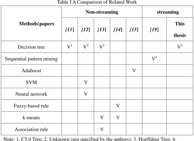
(18) analysis, and it has been widely applied to financial analysis. ARIMA was extended from autoregressive moving average (ARMA) [9]. However, ARIMA hardly recognizes nonlinear pattern. Hence, Pai and Lin proposed a hybrid method which integrated ARIMA model and support vector machine (SVM) to forecast stock price [10]. SVM is a data mining technique which is able to handle non-linear problem. By the empirical result, Pai and Lin thought that hybrid method improves prediction performance of each single model, and they found that simple combination of two best models (single ARIMA and single SVM) did not give the best performance.. 立. 政治大. 2.2 Non-Streaming Data Mining Techniques for Financial Data Analysis. ‧ 國. 學. In this section, we briefly review related work which predict stock or futures by their. ‧. transactions and give a comparison of related work, as shown in Table I. In Table I, a column. sit. y. Nat. represents a paper related to the topic of this thesis and a row represents a data mining. io. er. technique. A cell of the table indicates that if the paper corresponding to a column uses the. al. v i n upper right corner indicates thatC thehpaper decision tree (and so do U e n g[11]c uses h i non-streaming n. method corresponding to a row. If yes then it is marked by “V”. For example, the cell in the. the papers [12] and [13]) and the second right cell in the second row indicates that the paper [13] uses sequential pattern mining. For decision tree, we listed various versions used in related work. According to Table I, we can see that the popular methods include decision tree, Support Vector Machine (SVM), and neural network.. 7.

(19) Table I A Comparison of Related Work Non-streaming. streaming. Methods\papers. This [11]. [12]. [13]. [14]. [15]. [19] thesis. V1. Decision tree. V2. V1. V3 V4. Sequential pattern mining Adaboost. V. SVM. 立. V. Fuzzy-based rule. 學. ‧ 國. Neural network. 政V 治大 V V. Association rule. V. V. ‧. k-means. Nat. n. al. er. io. sit. y. Note: 1. C5.0 Tree; 2. Unknown (not specified by the authors); 3. Hoeffding Tree; 4. ICspan, IAspam.. i n U. v. Data of stocks or futures are naturally streaming data. When we use data mining. Ch. engchi. techniques designed for non-streaming data, it is important to transform a data stream into a set of data samples by using a time frame. In [11], 5-minute time frame is selected for TAIEX Futures forecasting. The paper uses C5.0 decision tree with two models: One is trained for rising or waiting, and it is named rising model; the other is trained for falling or waiting, and it is named falling model. These two models can be used with majority vote. To use majority vote, it would need a decision matrix, as the one shown in Table II. The row of the table is the decision of rising model, and the column is the decision of falling model. The cell of table is the joint decision given by majority vote. 8.

(20) Table II Decision Matrix Used in Paper [11] Rising\Falling. Waiting. Falling. Waiting. Waiting. Falling. Rising. Rising. Waiting. Paper [12] compares methods for forecasting Taiwan IC stocks. It compares SVM, SVM with Genetic Algorithm (GA-SVM), decision tree, and Back-Propagation Network. 治政 (BPN). Differing from other papers, it trains a model by大 financial indexes of accounting rather 立 than the records of transactions. ‧ 國. 學. Paper [13] uses data mining techniques such as classification, clustering, and. ‧. association rule to forecast the trend of stocks in the future. It analyzes the financial account of a company, and in order to examine whether the stock of a company is worth to hold, it. y. Nat. er. io. sit. uses C5.0 decision tree to train models.. Paper [14] uses TSK fuzzy model for forecasting rather than classifying the TAIEX.. n. al. Ch. i n U. v. Combining clustering method, TSK fuzzy model is better than BPN and multiple regression. engchi. analysis for forecasting TAIEX in the paper. The data types in the paper are technical indexes which are statistical or calculated information of transactions. Because there are many technical indexes, factor selection is a problem discussed in the paper. Using the groups of data clustered by K-means, the paper sets up simplified fuzzy rules and trains the parameters. Paper [15] designs a TAIEX Futures intra-day trading system, using Adaptive Boosting (Adaboost). The data source is based on technical indexes of TAIEX and the size of time frame used in the paper is 1 minute. The paper uses several methods combined with Adaboost to train models. 9.

(21) 2.3 Data Streaming Mining Techniques for Financial Data Analysis 2.3.1 Concept Drift Analysis Concept drift is a problem that the old static model can’t deal with new coming instances, and it often occurs in long term mining. So concept drift may exist not only in data stream mining but non-streaming data mining. However, concept drift forms its problem in common when processing data stream mining.. 政治大 Futures, which is traded by Sydney Futures Exchange and based on All Ordinaries Index, and 立 Harries and Horn used general decision tree algorithms to classify Share Price Index. ‧ 國. 學. they proposed a strategy that dealt with concept drift by classifying only new data instances that are similar to those used in training [16].. ‧. In paper [17], Pratt and Tschapek proposed Brushed Parallel Histogram for visualizing. sit. y. Nat. concept drift [17]. They used 500 Standard and Poor’s listed stocks during 2002 and concluded. io. er. that “a machine learning assumption of stationary would be unsupported by the data and that. al. v i n C h and Black discussed In paper [18], Marrs, Hickey e n g c h i U the impact of latency on online n. static market prediction models may be fragile in the face of drift” [17].. classification when learning with concept drift. Latency corresponds to the duration of the recovery from concept drift. Moreover, they proposed an online learning model for data streams, and they proposed an online learning algorithm, which is based on the model, to evaluate the impact of latency. Furthermore, they showed that different types of latency have different impacts on the recovering accuracy.. 2.3.2 Data Stream Mining Techniques Paper [19] discusses sequential pattern miming techniques. It uses five ordinal labels as. 10.

(22) patterns of the change of the stock price: falling, few falling, unchanged, few rising and rising. The inputs in the paper are multiple data streams consisting of the five types of patterns from various stocks. The paper uses two sequential pattern mining techniques, namely ICspan and IAspam, which can discover common sequential patterns from multiple inputs. However, ICspan and IAspam do not follow requirements for data streams. Using non-streaming data mining methods on streaming data will have to face the problem of concept drift, which will decrease the accuracy as time passes. It is necessary to adjust the. 政治大. built model appropriately. In this thesis, we apply data stream mining techniques on TAIEX. 立. Futures data with MOA [2], which offers classification and clustering algorithms for data. ‧ 國. 學. streams and also evaluation strategies to help its users appropriately validate the built models. In paper [20], Sun and Li proposed an expert system to predict financial distress and used. ‧. instance selection for handling concept drift, including full memory window, no memory. y. Nat. sit. window, fixed window size, adaptive window size, and batch selection. Sun and Li evaluated. n. al. er. io. the system by financial statements of companies from Chinese Stock Exchange (CSE) and. i n U. v. recognized the company being in financial distress if it was specially treated by CSE. They. Ch. engchi. reported that some methods performed better than did others that only learn stationary models. Moreover, they stated that full memory and no memory windowing methods were usually not good at dealing with concept drift but good at detecting concept drift and the type of concept drift. However, Sun and Li did not indicate what types of concept drift exist or how to decide the types of concept drift. In paper [21], the author proposed On-Line Information Network (OLIN), an online classification system. OLIN deals with concept drift by adjusting the window size of training data and the number of coming instances between two model re-constructions.. 11.

(23) CHAPTER 3 DATA STREAM MINING 3.1 Introduction to Data Stream Mining. 政治大. Generally speaking, data mining problems could be divided into three categories,. 立. namely classification, clustering, and association rule. Classification is the problem whose goal. ‧ 國. 學. is to develop a model that can automatically classify coming instances into target classes. The model was trained by a given set of training instances, and a training instance contains values. ‧. for various attributes and is attached with a correct class label. If the number of classes in the. y. Nat. sit. data is 2, e.g. positive and negative, we call the problem a binary-class, or simply binary,. n. al. er. io. classification problem. We call it multiple-class classification problem if the number of classes. i n U. v. is larger than 2. Clustering is defined as the problem whose goal is to develop a model that can. Ch. engchi. partition the whole data set into various subsets or groups. The differences between these two problems include 1) classification needs to learn a model but clustering does not and 2) classification needs pre-specified class labels but clustering does not. Non-streaming data mining algorithms, such as C4.5 [22], ID3 [23], Repeated Incremental Pruning to Produce Error Reduction (RIPPER) [24], K-Nearest Neighbors (KNN) [25], Support Vector Machine (SVM) [26] and Adaptive Boosting (AdaBoost) [27], these algorithms store all instances in memory for training. Sometimes, these algorithms must be reconstructed when updating a built model with new instances. Some algorithms could be used in time series analysis. However, when processing an online task which usually includes 12.

(24) a series (rather than a set) of instances, non-streaming data mining algorithm will. require. more and more memory and time in order to store and process more and more instances. Moreover, an online task may need to update a model. Otherwise, using an old model to classify new instances may significantly decrease the classification performance. Data stream mining algorithms are designed to perform incremental learning, i.e. they can update models without reconstructing models. Furthermore, they do not store and keep all instances in memory all the time. These algorithms read instances into memory, update. 政治大. corresponding statistics, and then remove the instances from memory. Hence, these. 立. algorithms use a limited amount of memory and use less time because they do not need to. ‧ 國. 學. reconstruct models.. In summary, data stream mining takes streaming data as input, and streaming data. ‧. should be analyzed in a reasonable amount of time and by using a limited amount of memory.. y. Nat. er. io. sit. 3.2 Concept Drift. al. v i n underlying data distribution, andC thehtarget depends on hidden context. It assumes that e nconcept gchi U n. Concept drift is an important issue for data stream mining. Concept presents the. all the data samples are fetched from a true underlying data distribution in the real world. When hidden context changes, the distribution of data samples will also change, and the target classes of data may also change. If the concept keeps the same, the distribution is stationary. When the underlying data distribution changed, it is called concept drift [28]. Concept drift has an impact on data analysis. The impact is amplified under online learning. Concept drift causes significant decreasing of accuracy. When the target concept changes, the old model may make wrong decisions for instances that are similar to instances which the old model is built on but with different class labels. Hence, updating is necessary 13.

(25) when concept drift occurs. There are four types of concept drift, as shown in Figure 1. Every row of figure shows a kind of types of concept drift. The distribution of color of an object in a row stands for the main concept. Different color distribution in a row means that concept changed by time. For example, the first row of Figure 1 shows sudden concept drift. Color distribution of 3rd object and 4th object are different, so they are different concept data. This process is called concept drift and because the concept changes suddenly, so this type is sudden.. 立. 政治大. ‧. ‧ 國. 學. n. er. io. sit. y. Nat. al. Ch. engchi. i n U. v. Figure 1. The four types of concept drift (reproduced from [29]) Note: The distribution of color of each data graph means a concept.. Sudden concept drift means that a concept jumps to another concept suddenly. Gradual concept drift and incremental concept drift mean that a concept move to another concept step by step. The difference between them is that incremental concept drift transfers to another. 14.

(26) concept directly. Reoccurring concept drift means that concept drift repeatedly appears in different points in time. Bifet et al. categorized the strategies used to handle different types of concept drift into four categories [29], as listed below. . Detector method: It uses variable-length windows and uses a new model when the corresponding detector is triggered. This method is suitable for dealing with sudden concept drift.. . 政治大. Forgetting method: It uses fixed-length windows and only processes data. 立. contained in a window, or it uses strategy that gives higher weights to new. ‧ 國. 學. instances. This method is suitable for dealing with sudden concept drift. . Contextual method: It uses dynamic integration or meta-learning strategy, and it. ‧. makes a decision by referring to results of sub-classifiers of an ensemble. This. y. Nat. n. al. er. Dynamic ensemble method: It uses adaptive fusion rules, and it makes decisions. io. . sit. method is suitable for dealing with reoccurring concept drift.. i n U. v. by weighted voting. This method is suitable for dealing with gradual and. Ch. incremental concept drift.. engchi. 3.3 MOA: A Data Stream Mining Tool Massive Online Analysis, MOA, is proposed by Bifet et al [2]. It is based on Waikato Environment for Knowledge Analysis, WEKA [3], and written in Java (an object-oriented and cross-platform programming language), and it supports a Graphical User Interface (GUI) and a command line interface. MOA offers a large set of functions to control the data mining process for data streams. For evaluation, MOA offers Prequential Evaluation, which tests each instances first and then trains a model using them; and it also offers Periodic Held Out Test, which tests 15.

(27) instances by a (static) trained model and outputs results for the evaluation period. For controlling data, MOA includes artificial data generation functions and, of course, it supports the use of data provided by users.. 3.4 Data Stream Mining Algorithms In this section, we introduce some data stream mining algorithms provided by MOA.. 3.3.1 Naïve Bayes. 治政 Naïve Bayes is one of the most popular algorithms 大in the field of data mining [30], and 立 it could be used in data stream mining. A Naïve Bayes classifier assumes that attributes are ‧ 國. 學. conditional independent. When classifying a given instance, it chooses the class label. ‧. corresponding to the highest probability. This model needs only statistical information so that there is no need to store all instances.. sit. y. Nat. io. n. al. er. 3.3.2 Hoeffding Tree. i n U. v. Hoeffding Tree [31] is a tree-base classification algorithm for data stream. The central. Ch. engchi. part of the algorithm is that splitting a node by choosing an attribute value such that the grade of the best attribute value is better than the one of the second when difference of the two grades is more than the Hoeffding bound. The grading function is information gain. With Hoeffding bound, the algorithm can match the requirements of data stream mining.. 3.3.3 Hoeffding Adaptive Tree There is another version of Hoeffding Tree used in this thesis -- Hoeffding Adaptive Tree [32][33], which is for adaptive parameter-free learning from evolving data streams. A data stream is an ordered sequence and the order is sensitive to time. In data stream miming, there 16.

(28) are three central problems to be solved and they are listed below: . What to remember (i.e. keep in memory)?. . When to upgrade the built model?. . How to upgrade the built model?. The above problems will be dealt with the following functions: . Window to remember recent samples.. . Methods for detect the change of data distribution.. . Methods for updating estimations for statistics of the input.. 政治大. 立. These three functions suggest a system to contain three modules: estimator, memory, and. ‧ 國. 學. change detector. Hoeffding Adaptive Tree is from Hoeffding Window Tree [32] which uses a window for Hoeffding tree. When change detector issues an alarm on a node of a tree, the. ‧. algorithm will create a new alternative Hoeffding Tree for the node, and it replaces the original. y. Nat. sit. sub-tree on the node with the alternative tree if the accuracy of the alternative tree is higher.. n. al. er. io. However, deciding the optimal size of the window requires sufficient background knowledge.. i n U. v. Hoeffding Adaptive Tree places instances of estimators of frequency statistics at every node. Ch. engchi. instead of setting the window size for Hoeffding Window Tree. Consequently, Hoeffding Adaptive Tree will evolve, and it needs no parameters for window size.. 3.3.4 Drift Detection Method In paper [34], Gama et al. proposed Drift Detection Method (DDM) to detect concept drift, and the method works in the following way: It calculates the minimum error rate of the model, denoted as 𝑝𝑚𝑚𝑚 , and the standard deviation, denoted as 𝑠𝑚𝑚𝑚 . Given a parameter α, for. the i-th data instance, DDM is at the warning level if 𝑝𝑖 + 𝑠𝑖 > 𝑝𝑚𝑚𝑚 + 2𝛼 ∗ 𝑠𝑚𝑚𝑚 . DDM is at. the drift level if 𝑝𝑖 + 𝑠𝑖 > 𝑝𝑚𝑚𝑚 + 3𝛼 ∗ 𝑠𝑚𝑚𝑚 . When DDM is at the warning level, it trains a new 17.

(29) classification model by using new data instances, and it replaces the old model with the new one if it moves to the drift level. DDM can handle sudden concept drift.. 3.3.5 Early Drift Detection Method In paper [35], Baena-García et al. proposed Early Drift Detection Method (EDDM) as an enhancement of DDM. EDDM is able to detect the presence of gradual concept drift. It works similarly to DDM but, instead of the error rate, EDDM considers the interval between two. 政治大 probability that concept drift occurs. 立. errors (i.e. incorrect classifications or predictions). The smaller is the interval, the higher is the. ‧ 國. 學. 3.3.6 Accuracy Weighted Ensemble. ‧. An ensemble is a group of sub-classifiers that provide collective intelligence by voting or other way, and evolving ensembles can be used to deal with concept drift. For example, we can. y. Nat. er. io. sit. use a chunk of data instances whose size is constant to train a sub-classifier. After training a number of sub-classifiers, we only use top-K best sub-classifiers to vote for overall. n. al. Ch. i n U. v. classifications. Every sub-classifier has its own weight calculated using the mean square error. engchi. rate, and its weight is updated when a new chunk comes. However, a new chunk of data instances will not be used to re-train the existing sub-classifiers, so these sub-classifiers may not be able to know that the underlying data distribution has changed. Accuracy Weighted Ensemble (AWE) [36] is one of the implementations for the above strategy. AWE uses a chunk under a given size to train a corresponding sub-classifier and calculates its weights by the distance between two minimum mean square errors for evaluation and expectation. The trained sub-classifier is static and will not be updated by a new chunk.. 18.

(30) 3.3.7 Accuracy Update Ensemble Accuracy Updated Ensemble (AUE) [37] improved AWE by updating sub-classifiers whenever their weights are larger than a threshold for the coming of every new chunk. Moreover, AUE uses a different way to calculate weights of sub-classifiers. AWE and AUE require an important parameter -- chunk size. However, the best chunk size should be evaluated beforehand so that AWE and AUE are not so easy to be applied to online tasks. Moreover, the best chunk size perhaps is not fixed but changes as time passes. Hence, in this thesis we propose. 治政 a method that can automatically adjust the chunk size. 大立. ‧. ‧ 國. 學. n. er. io. sit. y. Nat. al. Ch. engchi. 19. i n U. v.

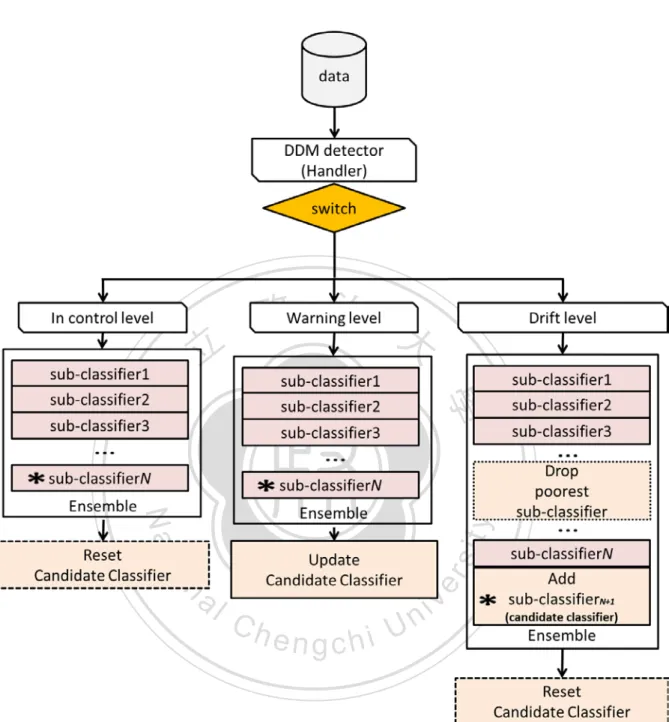
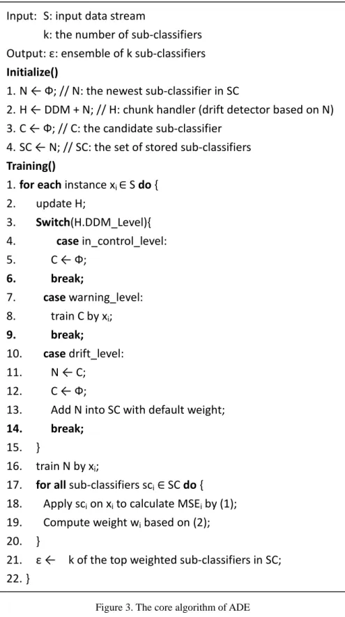
(31) CHAPTER 4 ADAPTIVE DRIFT ENSEMBLE In our experiments, we found that DDM can significantly improve accuracy no matter. 政治大 in the TAIEX Futures data. In the work presented in this chapter, our goal is to investigate the 立. what algorithm we used to build a single classifier. We concluded that there exists concept drift. ‧ 國. 學. types of concept drift existing in the TAIEX Futures data. We propose an ensemble based method, which contains static sub-classifiers that sufficiently reflect the corresponding. ‧. concepts. By observing changes of relative weights of sub-classifiers, we discover that a. y. sit. io. er. Futures data.. Nat. concept occurs repeatedly. In the other words, reoccurring concept drift exists in the TAIEX. al. v i n C hcore algorithm of U different drift detection levels. The e n g c h i ADE, presented in Figure 3, works as n. Figure 2 presents the flowchart of Adaptive Drift Ensemble (ADE), giving details for. follows: Initially, it resets or initializes the newest or current sub-classifier and employs DDM. In training, for each coming instance, it updates the DDM detector (handler) and determines the current level, which could be the control level, warning level, or drift level. ADE uses the coming instance to update the DDM detector, which is the current sub-classifier (marked by asterisk in Figure 2) with DDM. The next step depends on the level suggested by the DDM detector. If the DDM detector suggests the control level, ADE uses the new data instance to update the current sub-classifier and resets the candidate classifier. If the DDM detector suggests the warning level, it updates the candidate classifier. If the DDM detector suggests the 20.

(32) drift level, ADE adds the candidate classifier to the ensemble and sets it as the current sub-classifier. Then ADE trains the current sub-classifier by using the coming instance, and it updates weights of sub-classifiers in the ensemble by Equations (1) and (2), which are from AUE. Finally, if the number of sub-classifiers exceeds the limit, ADE drops the one that performs the worst, and it returns top k sub-classifiers according to their weights. 𝑀𝑆𝐸𝑚 =. 1 ∑ �1 |𝑥𝑖 | (𝑥,𝑐)∈𝑥𝑖. 1. 2. − 𝑓𝑐𝑚 (𝑥)� , 𝑀𝑆𝐸𝑟 = ∑𝑐 𝑝(𝑐)(1 − 𝑝(𝑐))2. 𝑤𝑚 = (𝑀𝑆𝐸 +𝜖) 𝑖. 立. 政治大. ‧ 國. x: an instance of the chunk. ‧. c: a chunk. (2). 學. i: the order in the series of instances of the chunk. y. Nat. w: weight of sub-model. n. er. io. al. sit. ϵ: a value which is limited to 0. Ch. engchi. 21. i n U. (1). v.

(33) 立. 政治大. ‧. ‧ 國. 學. n. er. io. sit. y. Nat. al. Ch. engchi. i n U. v. Figure 2. The flowchart of the handler (DDM detector) of ADE. 22.

(34) Input: S: input data stream k: the number of sub-classifiers Output: ε: ensemble of k sub-classifiers Initialize() 1. N ← Ф; // N: the newest sub-classifier in SC 2. H ← DDM + N; // H: chunk handler (drift detector based on N) 3. C ← Ф; // C: the candidate sub-classifier 4. SC ← N; // SC: the set of stored sub-classifiers Training() 1. for each instance xi ∈ S do { 2. update H; 3. Switch(H.DDM_Level){ 4. case in_control_level: 5. C ← Ф; 6. break; 7. case warning_level: 8. train C by xi; 9. break; 10. case drift_level: 11. N ← C; 12. C ← Ф; 13. Add N into SC with default weight; 14. break; 15. } 16. train N by xi; 17. for all sub-classifiers sci ∈ SC do { 18. Apply sci on xi to calculate MSEi by (1);. 立. 政治大. ‧. ‧ 國. 學. n. er. io. sit. y. Nat. al. Ch. engchi. i n U. v. 19. Compute weight wi based on (2); 20. } 21. ε ← k of the top weighted sub-classifiers in SC; 22. } Figure 3. The core algorithm of ADE. 23.

(35) In order to set the chunk size of each sub-classifier adaptively and vary the number of data instances given to every sub-classifier for training, we use DDM as the base handler to calculate and adjust the chunk size. We put into a chunk the data instances collected before the drift level is triggered, and we use the chunk to train a sub-classifier. We use DDM because, according to our experimental results (in 5.2.2 and 5.2.3), EDDM is less stable than DDM. Although we use DDM, any concept drift detector would work as the base handler. EDDM was proposed to mainly handle gradual concept drift, and DDM was proposed to. 政治大. mainly handle sudden concept drift [35]. ADE could be built upon any concept drift detector.. 立. AUE trains a new sub-classifier with instances of a chunk and then adds it to an ensemble. ‧ 國. 學. if and only if the chunk is full. Before a chunk is full, the coming instances do not contribute to training but only to updating weights of sub-classifiers. As a result, AUE can only vote for a. ‧. new coming instance by using old sub-classifiers. AUE has a delayed reaction for concept drift.. y. Nat. sit. Such a condition is related to latency learning. According to the paper [18], we know that. n. al. er. io. latency causes slow recovery when concept drift occurs. To address this problem, ADE not only. i n U. v. updates weights but also trains the current sub-classifier by using every coming instance immediately.. Ch. engchi. A chunk of instances is used to train a sub-classifier in AWE and AUE, so it is important to determinate the chunk size in advance. However, the best chunk size may not constantly be the same. We use a handler in an ensemble to determine the chunk size for two reasons: One is that each sub-classifier can represent the corresponding concept, and the other is that the handler can adjust the chunk size automatically. The size is the difference in terms of the number of data instances between two drift levels that occur. In summary, we improve AUE from three aspects. First, we use a single classifier, which is based on the newest sub-classifier of ensemble, with DDM to determine the chunk size. 24.

(36) Second, we keep old sub-classifiers without updating them. Third, we update current sub-classifier (the newest one) for every new data instance instead of waiting until the chunk is full (when the drift level occurs).. 立. 政治大. ‧. ‧ 國. 學. n. er. io. sit. y. Nat. al. Ch. engchi. 25. i n U. v.

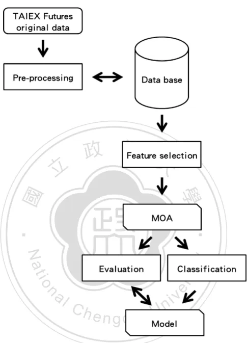
(37) CHAPTER 5 EXPERIMENTS 5.1 Setup. 政治大. The following includes preparation for experiment and result of applying data stream. 立. mining techniques on prediction of TAIEX Futures. We observed the results and discovered. ‧ 國. 學. that concept drift existed in TAIEX Futures market. The next chapter will discuss concept drifts more detailed.. ‧. We describe in detail the experiments whose goal is to evaluate the performance of the. y. Nat. n. al. er. io. experiments.. sit. algorithms mentioned earlier on the TAIEX Futures data. Figure 4 presents the procedure for. Ch. engchi. 26. i n U. v.

(38) 立. 政治大. ‧. ‧ 國. 學. n. er. io. sit. y. Nat. al. Ch. engchi. i n U. v. Figure 4. The procedure for experiments The transactions of TAIEX Futures were used as input data. In order to filter structure format, we stored the semi-structure transactions into database. Before using data stream mining tool, we selected a subset of features by heuristic. We conduct experiments by using the toolkit MOA [2], which is based on WEKA [3]. MOA offers a rich set of functions for data stream mining. MOA offers Prequential Evaluation that tests instances first and then uses them to train a model. 27.

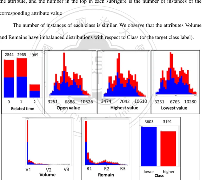
(39) For baseline experiment, TAIEX Futures data used in experiments, downloaded from Taiwan Stock Exchange Corporation web, includes transaction between January 1st in 2000 and December 31th in 2011, and the size of the time frame is set to 1 day. In order to train a model that can be used in the future, we remove all absolute timestamps and instead use relative timestamps, because absolute timestamps will not occur in the future. Labeling also becomes a problem since we do not have real settlement values for futures. So, we label each record with a closest value. Furthermore, to avoid confusion, we remove. 政治大. instances having 0 on the volume attribute.. 立. The attributes of data are listed below: Related Time: The number of months from the trading date to the due date.. . Open Value: The opening price of a trading day.. . Close Value: The closing price of a trading day.. . Highest and Lowest Value: The highest and lowest price traded in a trading day.. . Volume: How many transactions of a trading day.. . Settlement Value: The settlement price of a trading day.. . Remains: How many remaining contracts in a trading day.. . Last Buy: The last price to buy at close time in a trading day.. . Last Sell: The last price to sell at close time in a trading day.. . Trading Time: In the format of Year/Month/Day.. . Class: Higher or lower, compared to the closing price of the final settlement day. ‧. ‧ 國. 學. . n. er. io. sit. y. Nat. al. Ch. engchi. i n U. v. with the close price of a trading day. Currently we select attributes by heuristics, and using some feature selection algorithms or statistical approaches will be part of our future work. Furthermore, we remove attributes that are directly related to the class label. For example, we use Close Value in the settlement day to 28.

(40) tag the class label, so we remove it in the experiments. We also select attributes through experiments. Consequently, after testing some subsets of these attributes, we decide to use only Relative Timestamps, Open Value, Highest Value, Lowest Value, Volume, Remains, and Class. The distributions of attributes are shown in Figure 5. Each subfigure in Figure 5 corresponds to an attribute. In the bottom is the attribute name. The x-axis is the set of values of the attribute, and the number in the top in each subfigure is the number of instances of the corresponding attribute value. 政治大. The number of instances of each class is similar. We observe that the attributes Volume. 立. and Remains have imbalanced distributions with respect to Class (or the target class label).. ‧. ‧ 國. 學. n. er. io. sit. y. Nat. al. Ch. engchi. i n U. v. Figure 5. Distribution of each attributes. Note: V1 = 1-6409, V2 = 134589-140998, V3 = 275587-281996, R1 = 4-3677, R2 = 36743-40417, and R3 = 77156-80830.. 29.

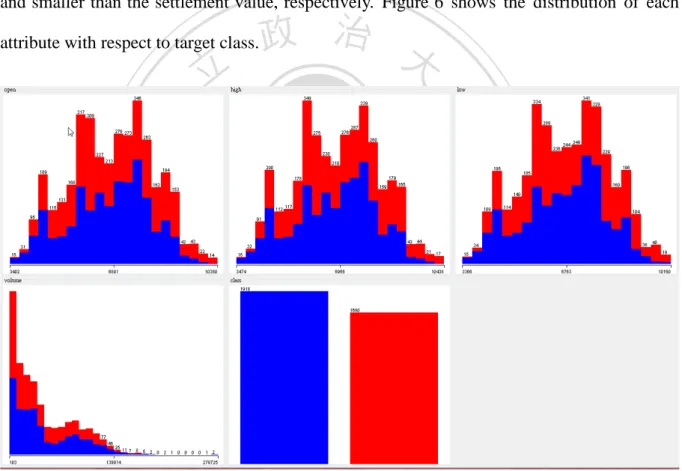
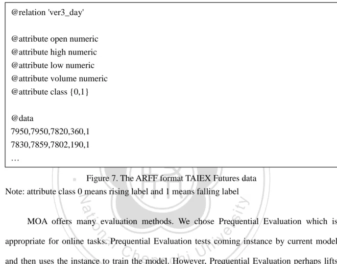
(41) For other experiments, in order to get more detailed granularity of time frame and more coverage of time duration of trading, we used only Open Value, Highest Value, Lowest Value, Volume and Class. The TAIEX Futures data used in experiments include transactions recorded in the time period starting from July 22nd, 1998 to October 31st, 2012. We remove all absolute timestamps in order to train classification models that can be used in different time frames. For every data instance, we set the class label as positive and negative when Close Value is larger and smaller than the settlement value, respectively. Figure 6 shows the distribution of each attribute with respect to target class.. 立. 政治大. ‧. ‧ 國. 學. n. er. io. sit. y. Nat. al. Ch. engchi. i n U. v. Figure 6. Distribution of each attribute Note: From left to right on the up side is Open Value, Highest Value and Lowest Value; from left to right on the down side is Volume and Class.. MOA accept many kinds of data format. We generated ARFF file as input after pre-processing. ARFF format is CSV file which attaches attribute information on the head of 30.

(42) file. Except for target class and Related time, all attributes are set as numerical type. For example, our data is shown as Figure 7. @relation 'ver3_day' @attribute open numeric @attribute high numeric @attribute low numeric @attribute volume numeric @attribute class {0,1}. 立. ‧. ‧ 國. 學. @data 7950,7950,7820,360,1 7830,7859,7802,190,1 …. 政治大. sit. y. Nat. Figure 7. The ARFF format TAIEX Futures data Note: attribute class 0 means rising label and 1 means falling label. n. al. er. io. MOA offers many evaluation methods. We chose Prequential Evaluation which is. i n U. v. appropriate for online tasks. Prequential Evaluation tests coming instance by current model. Ch. engchi. and then uses the instance to train the model. However, Prequential Evaluation perhaps lifts accuracy in our case, because it tests instances immediately. In fact, the instances are labeled only after the final settlement day in the real world. Hence, Prequential Evaluation ignored the latency which is about 20 instances at most in our case.. 5.2 Results 5.2.1 Baseline In the experiment, we classify instances with the default settings. For Hoeffding Tree, the parameters settings include 95% confidence, information gain and 200 instances for grace 31.

(43) period. Additionally, 30 instances ignored for DDM. We mainly use Hoeffding tree (HT) [31] for evaluation and use Naïve Bayes (NB) as the control group. One of the reasons that we consider Naïve Bayes is that it is one of the most popular algorithms in the field of data mining [30] and it could be used in data stream mining. Furthermore, another major reason of using Naïve Bayes as the control group is that there are many references, such as [38][39][40][41], where Naïve Bayes is used in finance data mining. Nevertheless, using other algorithms as the control group will be part of our future work.. 政治大. We used prequential evaluation which uses the coming instance to test model and then. 立. to train the model. When model classifies an instance correctly, it was recorded as positive for. ‧ 國. 學. accuracy. The figures were painted by Microsoft Excel, and each point on figure stands for average of 173 instances. We present experimental results in Figure 8 and Figure 9, each of. ‧. which uses accuracy in percentage as the y-axis and timestamps as the x-axis. It is shown in. y. Nat. sit. Figure 8 that the three algorithms achieve the average accuracy higher than 50%. We also could. n. al. er. io. find that Hoeffding Tree and Hoeffding Adaptive Tree do not perform worse than Naïve Bayes.. i n U. v. If stability of the built model is the concern, Hoeffding Tree or Hoeffding Adaptive Tree would. Ch. engchi. be a better choice. Accuracy decreased at beginning for almost experiments. We think the reason is that empty model guesses a static class, and TAIEX fell during the time, but model guessed the wrong class.. 32.

(44) Hoeffding Tree. Hoeffding Adaptive Tree. Naïve Bayes. 90 80 70 60. 2011/7/1. 2011/1/1. 2010/7/1. 2010/1/1. 2009/7/1. 2009/1/1. 2008/1/1. 2007/7/1. 2007/1/1. 2006/7/1. 2006/1/1. 2005/7/1. 2005/1/1. 2004/7/1. 2003/7/1. 2003/1/1. 2002/1/1. 2001/7/1. 2002/7/1. Figure 8. Algorithms without DDM. ‧. ‧ 國. 2001/1/1. 2000/7/1. 立. 政治大. 學. 2000/1/1. 30. 2004/1/1. 40. 2008/7/1. 50. Note: The y-axis starts from 30.. y. Nat. er. io. sit. From Figure 8, we can have the following findings: Prior to 2002, Hoeffding Tree and Hoeffding Adaptive Tree perform equally well and better than does Naïve Bayes, and for each. n. al. Ch. i n U. v. of the three algorithms the accuracy decreases as time passes. Between late 2002 and early 2004,. engchi. the accuracy of Naïve Bayes increases as time passes and performs better than do the other two algorithms. Between late 2004 and mid-2006, all the three algorithms exhibited a trend of increasing accuracy, and Hoeffding Adaptive Tree performs the best among the three (and this demonstrates the “adaptive” feature of the algorithm). Between mid-2006 and mid-2008, the accuracy given by Naïve Bayes drops rapidly (and it goes back to its mid-2006 level in mid-2009), while the other two algorithms perform similarly and significantly better than does Naïve Bayes. Between late 2008 and mid-2009, the accuracy given by Hoeffding Adaptive Tree decreases while the other two algorithms show a trend of increasing accuracy. After mid-2009,. 33.

(45) Hoeffding Adaptive Tree shows a trend of increasing accuracy until mid-2010, while Hoeffding Tree shows a similar trend but Naïve Bayes shows a trend of decreasing accuracy. After mid-2010, all the three algorithms show a trend of decreasing accuracy, but after mid-2011, the accuracy given by Naïve Bayes increases as time passes. As shown in Figure 9, the accuracy given by Hoeffding Adaptive Tree with DDM is not as good as the accuracy given by others, because there are other estimators in Hoeffding Adaptive Tree. DDM uses a type II estimator [32], and Hoeffding Adaptive Tree uses a type IV. 政治大. estimator. Thus, when we compare Hoeffding Adaptive Tree in Figure 8 with other algorithms. 立. with DDM in Figure 9, we can observe that using a type IV estimator is not always better than. ‧ 國. 學. using a type II estimator.. ‧. Hoeffding Tree with DDM. sit. io. 80. er. 85. al. n. 75. Naïve Bayes with DDM. y. Nat. 90. Hoeffding Adaptive Tree with DDM. Ch. 70 65. engchi. i n U. v. 2011/7/1. 2011/1/1. 2010/7/1. 2010/1/1. 2009/7/1. 2009/1/1. 2008/7/1. 2008/1/1. 2007/7/1. 2007/1/1. 2006/7/1. 2006/1/1. 2005/7/1. 2005/1/1. 2004/7/1. 2004/1/1. 2003/7/1. 2003/1/1. 2002/7/1. 2002/1/1. 2001/7/1. 2001/1/1. 2000/7/1. 2000/1/1. 60. Figure 9. Algorithms with DDM Note: the y-axis starts from 60.. We did another experiment by using data which is only during current settlement month instead of tree trading months (we can trade different settlement month of futures in a day). 34.

(46) Figure 10 shows result of different algorithms. Hoeffding Tree performed almost as well as Naïve Bayes because Hoeffding Tree uses Naïve Bayes to classify instance on the leave. Hoeffding Adaptive Tree performed worse than others, though Hoeffding Adaptive Tree contains an adaptive window for concept drift. On average, Hoeffding Tree gives accuracy at 58.08, Hoeffding Adaptive Tree gives 56.81, and Naïve Bayes gives 58.21. For standard deviation, Hoeffding Tree gives 5.65, Hoeffding Adaptive Tree gives 7.01 and Naïve Bayes gives 5.84. Hoeffding Tree. 立. 85. Hoeffding Adaptive Tree. sit. 2011/7/1. 2011/1/1. 2010/7/1. engchi. v. 2010/1/1. 2006/7/1. 2006/1/1. 2005/7/1. 2005/1/1. 2004/7/1. 2004/1/1. 2003/7/1. 2003/1/1. 2002/7/1. 2002/1/1. 2001/7/1. 2001/1/1. 2000/7/1. 2000/1/1. Ch. i n U. 2009/7/1. er. al. n. 40. 2007/7/1. io. 45. 2007/1/1. 50. y. Nat. 55. 2009/1/1. 60. 2008/7/1. 65. 2008/1/1. 70. ‧. ‧ 國. 75. Naïve Bayes. 學. 80. 政治大. Figure 10. Baseline Note: Only current settlement month data, the y-axis starts from 40. Figure 11 shows result using DDM and data set as above. Algorithms with DDM performed better than Algorithms without DDM did. Hoeffding Tree with DDM performed worse than others. On average, Hoeffding Tree with DDM give accuracy at 71.39, Hoeffding Adaptive Tree with DDM gives 73.53 and Naïve Bayes with DDM gives 72.24. For standard deviation, Hoeffding Tree with DDM gives 3.87, Hoeffding Adaptive Tree gives 1.76 and 35.

(47) Naïve Bayes gives 1.75. Hoeffding Tree with DDM. Hoeffding Adaptive Tree with DDM. Naïve Bayes with DDM. 85 80 75 70. 2011/7/1. 2011/1/1. 2010/7/1. 2010/1/1. 2009/7/1. 2009/1/1. 2008/7/1. 2008/1/1. 2007/7/1. 2007/1/1. 2006/7/1. 2006/1/1. 2005/7/1. 2005/1/1. 2004/7/1. 2003/7/1. 2003/1/1. 2002/1/1. 2001/7/1. 2002/7/1. Figure 11. Algorithms with DDM. ‧. ‧ 國. 2001/1/1. 2000/7/1. 立. 學. 2000/1/1. 60. 2004/1/1. 政治大. 65. sit. y. Nat. Note: Only current settlement month data, the y-axis starts from 60.. io. n. al. er. 5.2.2 Drift Detection Method. i n U. v. We used different data set from the base experiment. For more detailed observation of. Ch. engchi. impact of DDM, we used data which is only during current settlement month and without Remains attribute which was used in base experiment. Figure 12 shows the result of DDM with different classification algorithms. Although we removed Remains attribute, there is no significant difference of average accuracy of DDM between two different subset of attribute and different coverage of time. On average, Hoeffding Tree with DDM gives accuracy at 71.39%, Hoeffding Adaptive Tree with DDM gives 73.53% and Naïve Bayes with DDM gives 72.24. For standard deviation of accuracy, Hoeffding Tree with DDM gives 6.09, Hoeffding Adaptive Tree with DDM give 5.66 and Naïve Bayes with DDM gives 7.34.. 36.

(48) 100. Hoeffding Tree with DDM. Hoeffding Adaptive Tree with DDM. Naïve Bayes with DDM. 95 90 85 80 75. 2012/8/1. 2012/1/1. 2011/6/1. 2010/11/1. 2010/4/1. 2009/9/1. 2009/2/1. 2008/7/1. 2007/5/1. 2006/10/1. 2006/3/1. 2005/8/1. 2005/1/1. 2004/6/1. 2003/11/1. 2002/9/1. 2002/2/1. 2001/7/1. 2000/12/1. 2000/5/1. ‧ 國. 1999/10/1. 1999/3/1. 立. 學. 1998/8/1. 60. 政治大. 2003/4/1. 65. 2007/12/1. 70. Figure 12. Algorithms with DDM. ‧. Note: Without Remains attribute 1998/7-2012/10, the y-axis starts from 60.. y. Nat. er. io. sit. 5.2.3 Early Drift Detection Method. We made experiment by Early Drift Detection Method which is provided by MOA. The. n. al. Ch. i n U. v. result was shown as Figure 13. We found the trends of result of DDM and EDDM are similar,. engchi. but EDDM made less shacking of accuracy, in other words, EDDM performed much stably. On average, Hoeffding Tree with EDDM gives accuracy at 72.45, Hoeffding Adaptive Tree with EDDM gives 72.89 and Naïve Bayes with EDDM gives 71.63. For standard deviation, Hoeffding Tree with EDDM gives 4.54, Hoeffding Adaptive Tree with EDDM gives 4.31 and Naïve Bayes with EDDM gives 5.00.. 37.

(49) 100. Hoeffding Tree with EDDM. Hoeffding Adaptive Tree with EDDM. Naïve Bayes with EDDM. 95 90 85 80 75 70. 2012/8/1. 2012/1/1. 2011/6/1. 2010/11/1. 2010/4/1. 2009/9/1. 2009/2/1. 2007/12/1. 2007/5/1. 2006/10/1. 2006/3/1. 2005/8/1. 2005/1/1. 2004/6/1. 政治大 2003/11/1. 2003/4/1. 2002/9/1. 2002/2/1. 2001/7/1. 2000/12/1. 立. 學. ‧ 國. 2000/5/1. 1999/10/1. 1999/3/1. 1998/8/1. 60. 2008/7/1. 65. Figure 13. Algorithms with EDDM. Note: Without Remains attribute 1998/7-2012/10, the y-axis starts from 60.. ‧. 5.2.4 Accuracy Weighted Ensemble. sit. y. Nat. io. er. AWE is evolving ensemble method. We used it for this experiment. Hoeffding Tree and. al. v i n C h Hoeffding TreeUwith AWE gives accuracy at 58.61, 14 shows result of AWE. On average, engchi n. Hoeffding Adaptive Tree performed a little better than Naïve Bayes when using AWE. Figure. Hoeffding Adaptive Tree with AWE gives 59.94 and Naïve Bayes with AWE gives 57.31. For standard deviation, Hoeffding Tree with AWE gives 6.96, Hoeffding Adaptive Tree with AWE gives 6.6 and Naïve Bayes with AWE gives 6.66.. 38.

(50) AWE Hoeffding Tree. AWE Hoeffding Adaptive Tree. AWE Naïve Bayes. 75 70 65 60 55. 2012/8/1. 2012/1/1. 2011/6/1. 2010/11/1. 2010/4/1. 2009/9/1. 2009/2/1. 2008/7/1. 2007/12/1. 2007/5/1. 2006/10/1. 2006/3/1. 2005/8/1. 2005/1/1. 2004/6/1. 2003/11/1. 2002/9/1. 2002/2/1. 2000/12/1. 2001/7/1. Figure 14. Algorithms with AWE. ‧. ‧ 國. 2000/5/1. 1999/10/1. 1999/3/1. 立. 學. 1998/8/1. 45. 2003/4/1. 政治大. 50. sit. y. Nat. Note: Without Remains attribute 1998/7-2012/10, the y-axis starts from 45.. io. n. al. er. 5.2.5 Accuracy Update Ensemble. i n U. v. AUE was improved from AWE, and AUE updates old sub-classifiers by new coming. Ch. engchi. instances. However, AUE performed little worse than AWE. Figure 15 shows result of AUE. On average, Hoeffding Tree with AUE gives accuracy at 57.87, Hoeffding Adaptive Tree with AUE gives 59.28 and Naïve Bayes with AUE gives 56.80. For standard deviation, Hoeffding Tree with AUE gives 6.99, Hoeffding Adaptive Tree with AUE gives 7.06 and Naïve Bayes with AUE gives 6.67.. 39.

(51) AUE Hoeffding Tree. 75. AUE Hoeffding Adaptive Tree. AUE Naïve Bayes. 70 65 60 55. 2012/8/1. 2012/1/1. 2011/6/1. 2010/11/1. 2010/4/1. 2009/9/1. 2009/2/1. 2008/7/1. 2007/12/1. 2007/5/1. 2006/10/1. 2006/3/1. 2005/8/1. 2005/1/1. 2004/6/1. 2003/4/1. 2001/7/1. 2000/12/1. 2002/2/1. Figure 15. Algorithms with AUE. ‧. ‧ 國. 2000/5/1. 1999/10/1. 1999/3/1. 1998/8/1. 學. 2002/9/1. 立. 45. 2003/11/1. 政治大. 50. sit. y. Nat. Note: Without Remains attribute 1998/7-2012/10, the y-axis starts from 45.. io. n. al. er. 5.2.6 Adaptive Drift Ensemble. i n U. v. For ADE, in experiments we use k=10 (the default value), i.e. there can be at most 10. Ch. engchi. active sub-classifiers in an ensemble. We transfer an absolute weight into a relative weight that is normalized from 0 to 1. We make an assumption that if the classification performance (e.g. accuracy) of a classifier is better than that of another then the classifier is able to reflect the current concept with a higher probability. Hence, when the relative weight of a sub-classifier is high, it indicates that the current concept (i.e. the underlying data distribution) is similar to, or the same as, the one that was used to train the sub-classifier. In the beginning, ADE trains a sub-classifier and adds a new sub-classifier to an ensemble when it is at the drift level. If the number of sub-classifiers is larger than 10 (as we use k=10), the sub-classifier that performs the worst will be dropped. 40.

(52) The total number of instances in the TAIEX Futures data is 3,598. We define the lifespan of a sub-classifier as the number of instances that it covers (or on which it is active). On average, a sub-classifier covers 1,043 instances when NB is used, and a sub-classifier covers 946 instances when HT is used. The standard deviation is 698 for NB and it is 732 for HT. Figure 16 shows the result of ADE. Hoeffding Adaptive Tree with ADE got bigger amplitude than others. On average, Hoeffding Tree with ADE gives 64.65 at accuracy, Hoeffding Adaptive Tree with ADE gives 64.65 and Naïve Bayes with ADE gives 63.29. For. 政治大. standard deviation, Hoeffding Tree with ADE gives 5.8, Hoeffding Adaptive Tree gives 7.5. 立. and Naïve Bayes with ADE gives 6.06.. ‧ 國. 學. ADE Hoeffding Tree. 75. n. al. er. io. 65. sit. y. Nat. 70. ADE Naïve Bayes. ‧. 80. ADE Hoeffding Adaptive Tree. 60. Ch. 55. engchi. i n U. v. Figure 16. Result of Adaptive Drift Ensemble Note: The y-axis starts from 50.. 41. 2012/8/1. 2012/1/1. 2011/6/1. 2010/11/1. 2010/4/1. 2009/9/1. 2009/2/1. 2008/7/1. 2007/12/1. 2007/5/1. 2006/10/1. 2006/3/1. 2005/8/1. 2005/1/1. 2004/6/1. 2003/11/1. 2003/4/1. 2002/9/1. 2002/2/1. 2001/7/1. 2000/12/1. 2000/5/1. 1999/10/1. 1999/3/1. 1998/8/1. 50.

(53) CHPATER 6 DISCUSSIONS 6.1 Impact of Concept Drift 6.1.1 Existence. 立. 政治大. We used classification algorithms with and without DDM which is drift detector for. ‧ 國. 學. experiments. The difference of results can be referred as impact of DDM. DDM is able to. ‧. handle concept drift which bring significant decreasing of accuracy [34]. We can say concept drift exists if algorithms with DDM perform better than algorithms without DDM at accuracy,. y. Nat. impact of concept drift is decreasing of accuracy.. n. al. Ch. er. io. sit. because the only impact is DDM which was designed for dealing with concept drift and the. i n U. v. The following is fetched from result of base experiment, comparing Figure 8 with. engchi. Figure 9; we observe that algorithms with DDM usually perform better than do those without DDM. Moreover, we can see from Figure 17 that the accuracy Hoeffding Tree with DDM is consistently higher than that of Hoeffding Tree without DDM. Similarly, we can see from Figure 18 that the accuracy of Naïve Bayes with DDM is consistently higher than that of Naïve Bayes without DDM. We think Hoeffding Adaptive Tree which contains a drift detector is not appropriate to combine with DDM which is another drift detector, so we did not give a comparison here. Therefore, we can accept that assumption that concept drift exists in the TAIEX Futures data.. 42.