合作式放大傳遞多輸入多輸出中繼系統之線性與非線性傳收機設計

(1)

國立交通大學

電機工程學系

博士論文

合作式放大傳遞多輸入多輸出中繼系統之

線性與非線性傳收機設計

Linear and Nonlinear Transceiver Designs in

Amplify-and-Forward MIMO Relay Systems

研究生：曾凡碩

指導教授：吳文榕

(2)

合作式放大傳遞多輸入多輸出中繼系統之線性與

非線性傳收機設計

Linear and Nonlinear Transceiver Designs in

Amplify-and-Forward MIMO Relay Systems

研究生：曾凡碩

Student:

Fan-Shuo

Tseng

指導教授：吳文榕博士 Advisor:

Dr.

Wen-Rong

Wu

國立交通大學

電機工程學系

博士論文

A Dissertation

Submitted to Institute of Communication Engineering

College of Electrical Engineering

National Chiao Tung University

in Partial Fulfillment of the Requirements

for the Degree of Doctor of Philosophy

in

Electrical Engineering

Hsinchu, Taiwan

(3)

合作式放大傳遞多輸入多輸出中繼系統

之線性與非線性傳收機設計

研究生: 曾凡碩指導教授: 吳文榕博士

國立交通大學

電機工程學系博士班

摘要

三節點放大傳遞多輸入多輸出中繼系統之傳收機設計包含兩種通訊鏈結 - 直接鏈結(direct link)與中繼鏈結(relay link)，及兩種前置編碼器 – 來源端前置編碼 (source precoder)與中繼端前置編碼(relay precoder)。在這種系統中，大部分的傳收機設計都只設計中繼前置編碼器，有些設計甚至只考量中繼鏈結以簡化最佳化過程。在本論文中，我們提出新穎的線性與非線性傳收機設計，其中來源端前置編碼與中繼端前置編碼是根據直接鏈結與中繼鏈結的通道資訊，合併最佳化設計。在本論文所探討的傳收機中，中繼端前置編碼為線性，傳送端前置編碼與接收機可為線性或非線性。具體而言，我們考量四種傳收機設計，第一種為線性來源端前置編碼、線性中繼端前置編碼與最小均方錯誤(minimum mean-squared error)接收機。第二種考量非線性來源端前置編碼、線性中繼端前置編碼與最小均方錯誤接收機之傳收設計，第三種為線性來源端前置編碼、線性中繼端前置編碼與非線性 QR 干擾消除接收機(successive-interference-cancellation)傳收設計，最

(4)

後一種為線性來源端前置編碼、線性中繼端前置編碼與非線性最小均方錯誤干擾消除接收機傳收設計。在所有考量的傳收機設計中，不管是線性或非線性，困難點在於其最佳化的成本函數為來源端前置編碼與中繼端前置編碼的非線性函數，並且為非凹曲線最佳化(convex optimization)，為了克服這個設計上的困難，我們提出不同以往的前置編碼結構與設計方法，使得原本的傳收機設計可轉換為凹曲線最佳化問題，因此可推導出解析解。最後，本論文進一步探討以服務品質 (quality-of-service)觀點的線性來源端前置編碼、線性中繼端前置編碼與線性最小均方錯誤接收機之傳收設計，並延伸前述所提及之設計方式，提出此問題的解析解，由模擬結果得知，相較於其他現有方法，所提出的傳收機架構有較好的效能表現。

(5)

Linear and Nonlinear Transceiver Designs

in Amplify-and-Forward MIMO Relay

Systems

Student: Fan-Shuo Tseng Advisor: Dr. Wen-Rong Wu

Institute of Communication Engineering

National Chiao Tung University

Abstract

The transceiver design in three-node amplify-and-forward (AF) multiple-input multiple-output (MIMO) relay systems involve two links, the direct and relay links, and two precoders, the source and relay precoders. Most existing methods only consider the design with a relay precoder, and some even ignore the direct link. In this dissertation, we propose new linear/nonlinear transceiver design methods taking the direct and relay links into account, and jointly optimizing the source and relay precoders. In our designs, the relay precoder is linear, and the source precoder and the receiver can be linear or nonlinear. Specifically, four scenarios are considered. The first is the design with a linear source precoder and a liner minimum-mean-square-error (MMSE) receiver, the second a nonlinear Tomlinson-Harashima source precoder and a linear MMSE receiver, the third a linear source precoder and a nonlinear QR successive-interference-cancelation (QR-SIC)

(6)

receiver, and the fourth a linear source precoder and a nonlinear MMSE-SIC receiver. All the designs, either the linear or nonlinear precoded systems, are difficult since the cost functions to be optimized are highly nonlinear functions of the source and relay precoders. Yet, the corresponding optimization problems are not convex. To overcome the difficulties, we propose new precoder architectures and methods such that the design problems can be translated into scalar-valued and convex optimization problems. And, the closed-form solutions can be obtained by the corresponding Karush-Kuhn Tucker (KKT) conditions. Finally, we consider the precoders design with quality-of-service (QoS) constraints. In the scenario, the linear precoder is used at the source and the MMSE receiver at the destination. Again, this problem is difficult and the optimization problem is not convex. We then extend the method proposed for the systems mentioned above to derive a closed-form solution. Simulation results show that the performance of the proposed transceiver design methods is significantly better than that of existing methods.

(7)

Acknowledgements

During the Ph.D. program, I would like to show my gratitude to many people. First, I would like to thank my advisor, Prof. Wen-Rong Wu, for his kindly guidance. He spends a lot of time in discussing the problems I encounter in my research, providing valuable suggestions, and teaching me how to write technical papers. In addition to academic research, he provides lots of resources in improving our English proficiency. Under his enthusiastic instruction, I learned not only how to do a research but also learned the optimistic study attitude. At this moment, I have to say Prof. Wu is the key person whom I am most grateful to in my studying life.

Second, I am grateful to all the members in Prof. Wu’s lab. for their valuable discussion and help in academic research including Fang Lee, Chao-Yuan Hsu, Hung-Dau Hsieh, Chun-Tao Lin, and so on. Especially, I would like to thank Chao-Yuan Hsu for his encouragement and help during the period of the Ph.D. program. Also, I would like to thank all my friends who ever encourage or help me, especially Shih-Wei Wang and Sin-Syun Li.

Finally, I would like to show my deep gratitude to my family, especially my best-loved wife, Kai-Wen Liang, and parents, Chien-Li Tseng and Jin-Ping Hung, for their support and encouragement in the Ph.D. program period.

(8)

(9)

List of Tables

2.1 Complexity of linear source and relay precoders (MMSE receiver). . . 23

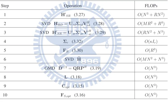
3.1 Computational Complexity of THP source and linear relay precoders (MMSE receiver). . . 43

3.2 Proposed water-filling algorithm solving (3.32) . . . 44

4.1 Computational Complexity of linear source and relay precoders (QR-SIC re-ceiver). . . 57

5.1 Complexity of linear source and relay precoders (MMSE-SIC receiver). . . 74

5.2 Source and relay precoders in the proposed nonlinear transceivers. . . 75

5.3 Optimizations of the source and relay precoders in the proposed nonlinear transceivers. 76

(14)

(15)

List of Figures

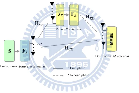
2.1 Linear source and relay precoded AF MIMO relay system with MMSE receiver. 24

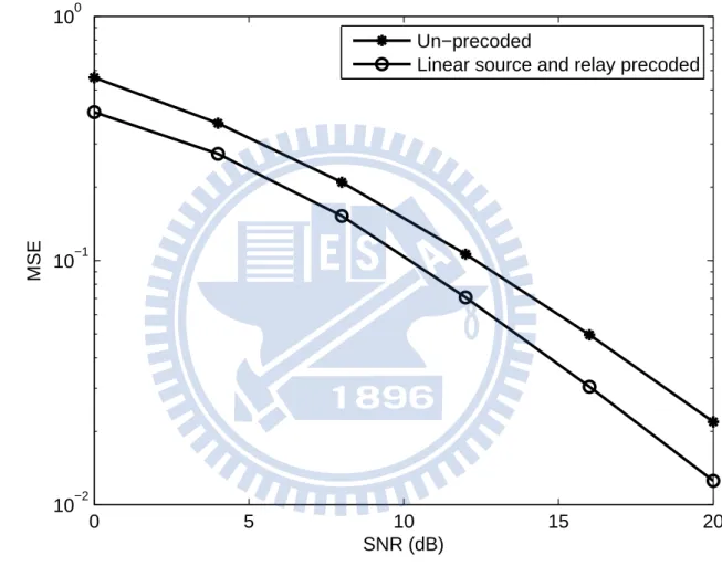
2.2 MSE performance comparison for un-precoded and linear source and relay pre-coded AF SISO-OFDM cooperative systems. . . 25

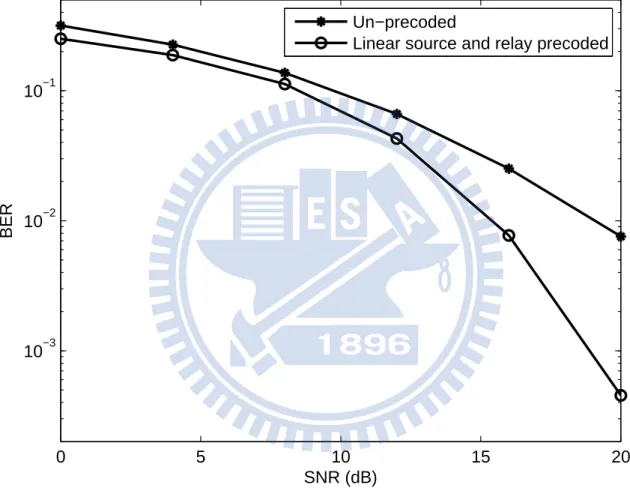
2.3 BER performance comparison for un-precoded and linear source and relay pre-coded AF SISO-OFDM cooperative systems. . . 26

2.4 MSE performance comparison for existing un-precoded/precoded and linear source and relay precoded AF two-hop MIMO relay systems. . . 27

2.5 BER performance comparison for existing un-precoded/precoded and linear source and relay precoded AF two-hop MIMO relay systems. . . 28

2.6 BER performance comparison for antenna selection [45] and linear source and relay precoded AF two-hop MIMO relay systems (L = 1 and N = R = M = 4). 29

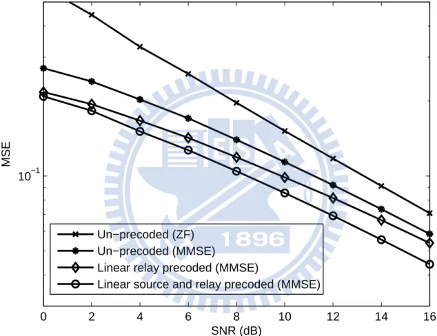
2.7 MSE performance comparison for existing un-precoded/precoded and linear source and relay precoded AF MIMO relay systems. . . 30

2.8 BER performance comparison for existing un-precoded/precoded and linear source and relay precoded AF MIMO relay systems. . . 31

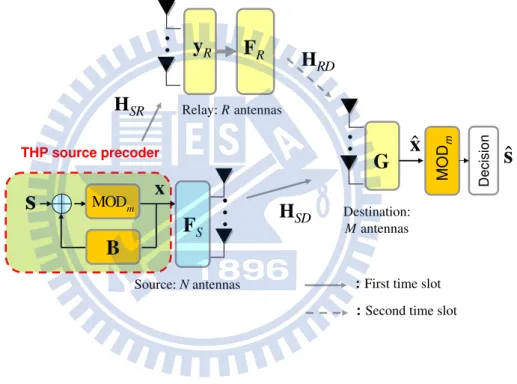
3.1 THP source and linear relay precoded AF MIMO relay system with MMSE receiver. . . 45

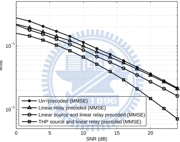
3.2 MSE performance comparison for existing precoded systems and THP source and linear relay precoded system with MMSE receiver. . . 46

(16)

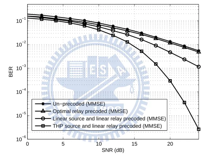
3.3 BER performance comparison for existing precoded systems and THP source and linear relay precoded system with MMSE receiver. . . 47

4.1 Linear source and relay precoded AF MIMO relay system with QR-SIC receiver. 61

4.2 BER performance comparison for linear source and relay precoded system with QR-SIC receiver and existing precoded systems (L = N = R = M = 4, SNRsr=SNRrd = 15 dB). . . . 62

4.3 BER performance comparison for linear source and relay precoded system with QR-SIC receiver and existing precoded systems (L = N = R = M = 4, SNRsr=15, SNRrd=0 dB). . . . 63

4.4 BER performance comparison for un-precoded, GMD source precoded, and linear source and relay precoded systems with ML receiver at the destination (L = N = R = M = 2, SNRsr=SNRrd=10 dB). . . . 64

4.5 BER performance comparison for linear source and relay precoded system with QR-SIC receiver and un-precoded systems (L = N = 4, R = M = 2 and 4-QAM is used for un-precoded systems; N = 4, L = R = M = 2 and 16-4-QAM is used for linear source and relay precoded system with QR-SIC receiver). . . 65

5.1 BLER performance comparison for un-precoded and precoded systems (16QAM,

N = R = M = 4, SNRsr=20, SNRsd=5 dB). . . . 79

5.2 BER performance comparison for un-precoded and precoded systems (16QAM,

5.3 BLER performance comparison for un-precoded and precoded systems (4-QAM,

5.4 BER performance comparison for un-precoded and precoded systems (4-QAM,

(17)

5.6 BER performance comparison for un-precoded and precoded systems (16QAM,

N = R = M = 4, SNRsd=5, SNRrd=20 dB). . . . 84

N = R = M = 2, SNRsd=5, SNRrd=20 dB). . . . 85

5.8 BLER performance comparison for un-precoded and precoded systems with imperfect CSIs (16QAM, N = R = M = 2, SNRsd=5, SNRsr=25 dB,

SNRrd=20 dB). . . . 86

6.1 Power consumption for proposed joint precoders method in two-hop MIMO relay system with σ2

sr = 0.0316 and σrd2 = 0.3162. . . . 103

6.2 Resultant MSE versus QoS with σ2

sr= 0.0316 and σ2rd= 0.3162. . . . 104

6.3 Power consumption for proposed joint precoders method in two-hop MIMO relay system with σ2

sr = 0.3162 and σrd2 = 0.0316. . . . 105

sr= 0.3162 and σ2rd= 0.0316. . . . 106

6.5 Resultant MSE performance of proposed precoders method in two-hop MIMO relay system with (ρ1, ρ2, ρ3, ρ4) = (0.008, 0.009, 0.01, 0.011). . . . 107

6.6 Power consumption for proposed joint precoders method in MIMO relay system with σ2

sr= 1, σ2rd= 1 and σsd2 = 0.1. . . . 108

sr= 1, σ2rd= 1 and σsd2 = 0.1 . . . . 109

6.8 Resultant MSE performance of proposed precoders method in MIMO relay sys-tem with (ρ1, ρ2, ρ3, ρ4) = (0.008, 0.009, 0.01, 0.011). . . . 110

(18)

(19)

Chapter 1 Introduction

D

Iversity is a commonly used technique to overcome the multipath channel fading effect in wireless communications. Existing diversity schemes include time diversity, frequency diversity, and spatial diversity. Among these schemes, the spatial diversity is particularly at-tractive. This is because it can combine with the other two diversity techniques with no time or bandwidth expansion [1]- [3]. The conventional way to obtain the spatial diversity is the use of multiple transmit or multiple receive antennas. When both multiple transmit and receive antennas are used, the system is referred to as a multiple-input multiple-output (MIMO) sys-tem [1]- [21]. The MIMO syssys-tem has been widely studied in the literature since it can enhance the diversity or spectral efficiency in an efficient way, [5]- [21]. However, due to shadowing, multipath fading, interference, and distance-dependent path losses, the link quality between the source and the destination in a wireless network may not be always good enough for reliable communication. The fundamentally linking problem greatly affects the transmission in wireless systems.

Recently, cooperative communication has been garnered great interest. In cooperative sys-tems, relays at some strong shadowing areas are deployed such that the signal from the source can be transmitted to the destination by the source-to-destination link (direct link) and the source-relay-destination links (relay links). With the additional relay links, the channel

(20)

qual-ity can be effectively improved, and the spatial diversqual-ity is implemented in a distributed way, referred to as distributed spatial diversity [22]- [49]. Various relay protocols have been proposed including amplify-and-forward (AF), decode-and-forward (DF), and compress-and-forward (CF) [22] [37]- [38]. In AF, the relays receive the signal from the source and retransmit it to the desti-nation with signal amplification only. Such a system is also called a non-regenerate cooperative system [41]- [43], [45]. In DF, the relays decode the received signals, re-encode the informa-tion bits, and then retransmit the resultant signals to the destinainforma-tion. The system is also called a regenerative cooperative system. One problem associated with the DF is that the decision errors can occur in the relays. The CF is a compromise structure between AF and DF where the received signals at the relays are estimated and compressed, and then re-transmitted to the des-tination. It is simple to see that the DF protocol requires a higher computational complexity and a larger processing delay at the relay nodes. In this dissertation, we only consider the AF-based cooperative system.

Recently, the MIMO technique was introduced to cooperative systems as a means for fur-ther performance enhancement. With the multiple antennas equipped at each node, a MIMO relay system is constructed [39]- [46]. Capacity bounds for a single-relay MIMO channel was first addressed in [39]. Similar to conventional MIMO systems, the precoding operation can be conducted in a MIMO relay system. For the MIMO relay systems, the relay precoder with AF protocol was first designed in [41]- [42] to enhance overall channel capacity. In most of those approaches, only the relay link is considered. It was shown that the capacity can be further increased if the direct link is taken into account [42]. Apart from the capacity, the link quality is another criterion has been considered. As well known, the precoder design is a transceiver de-sign problem which means a specific precoder is dede-signed for a specific receiver. In [43]- [44], a relay precoder was designed for a minimum mean-square error (MMSE) receiver. Precoding in multiple-relay MIMO systems was investigated in [44]. Note that the above works all address the spatial multiplexing scenario. Recently, the design for the transmission of a single data stream, referred to as beamforming, was also considered. For example, [46] derived the

(21)

op-timum source and relay beamformers using a maximum signal-to-noise-ratio (SNR) criterion. In the work, the optimum solution was derived for the relay-link-only system. In addition to beamforming, antenna selection in MIMO relay systems was also studied. With the MMSE cri-terion, an optimum selection scheme was developed in [45]. In this approach, only one antenna is selected at the source and the relay, respectively, for signal transmission.

As mentioned, in the precoders design for spatial multiplexing AF MIMO relay systems, the existing works only consider the precoder at the relay. Also, the direct link is frequently ignored [41]- [44]. In this dissertation, we consider the transceiver designs in three-node AF MIMO relay systems taking the direct and relay links into consideration, and jointly optimizing the source and relay precoders. Since the relay only amplifies its receive signal, a linear precoder is used in our study. We first consider the linear transceiver design where the linear precoder is used at the source and the MMSE receiver at the destination. The MMSE criterion is also used in [43]- [44]; however, only the relay precoder at the relay link is considered. With our formulation, it is found that the MMSE is a complicated function of precoding matrices, and a direct minimization is almost not possible to conduct. To overcome the difficulty, we pose some structural constraints on the precoders so as to diagonalize the MSE matrix in the cost function. With the precoders, we can then derive an MSE upper bound. Minimization with this upper bound, instead of the original MMSE, then becomes feasible. The proposed precoders can finally be computed via an iterative water-filling technique. Note that the MSE criterion to minimize is the total MSE of the multiplexed signal streams. With the specially designed structure, the proposed precoders can make the individual MSEs of all signal streams equal, indicating that the bit-error-rate (BER) of the proposed precoded system will be the minimal among all precoded systems with the same minimum total MSE [8].

To enhance the performance of the precoded system, we then use the nonlinear Tomlinson-Harashima precoder (THP) at the source and a MMSE receiver at the destination. As that in the linearly precoded MMSE system, the cost function is a highly nonlinear function of the source and relay precoders. Since the nonlinear THP is involved, the optimization problem

(22)

becomes more difficult. Even with the numerical method [51], finding the optimum solution is not a simple task. To overcome the problem, we propose to cascade a unitary precoder with the THP. The unitary precoder can not only simplify the optimization problem but also improve the MMSE performance. With the specially designed unitary precoder at the source, the primal decomposition approach [51], decomposing the original optimization problem into a master and a subproblem optimization problems, can be applied. The optimum source precoder in the subproblem can thus be derived as a function of the relay precoder. The problem is then similar to the precoding design in conventional MIMO systems [16] and the solution is readily obtained. The focus then becomes how to solve the master problem, in which the cost function is a function of the relay precoder only. Due to the nonlinear cost function, the relay precoder in the master optimization cannot be solved. We then propose an relay precoder structure and translate the relay optimization problem into a standard scalar-valued concave optimization problem. Using the Karush-Kuhn-Tucker (KKT) conditions, we then obtain a closed-form solution for the relay and source precoders.

An alternative to enhance system performance is to use a nonlinear receiver at the desti-nation. We then consider the system with a linear precoder at the source and a nonlinear QR successive-interference-cancelation (QR-SIC) or the MMSE-SIC receiver at the destination. In the transceiver design, the most desirable criterion to minimize is the BER. However, it is gen-erally acknowledged that a design minimizing BER is difficult to obtain. As an alternative, in this dissertation we propose to use the block-error-rate (BLER) instead of the BER as the de-sign criterion. For a MIMO system with a QR-SIC receiver, the precoder which can minimize the BLER has been solved by the geometric mean decomposition (GMD) technique [6],[7]. We then extend its use in AF MIMO relay systems to design the source and relay precoders, jointly. Although the AF MIMO relay system can be formulated as a general MIMO system and the GMD criterion can be easily applied, the cost function is a highly nonlinear function of the source and relay precoders. A direct optimization of such a function turns out to be infeasible. Fortunately, the GMD method allows us to express the source precoder as the

(23)

func-tion of the relay precoder. As a result, the two-precoder design problem can be reduced to a single-precoder problem. Similar to the approach used in the THP precoded system, we ap-ply the primal decomposition to translate the problem to a standard scalar convex optimization problem. The closed-form solutions for the source and relay precoders can then be obtained. It is noted here that GMD can also maximize a lower bound of channel’s free distance [12]. As known, the free distance is the metric used in the maximum likelihood detector (MLD). So, it is expected that the proposed precoders can also improve the performance of the MLD1_{. As well}

known, a precoded MIMO system with the MMSE-SIC receiver outperforms that with QR-SIC receiver. We can assert that the same result can be obtained for MIMO relay systems. For MIMO systems, the precoder with the MMSE-SIC receiver can be solved by the uniform chan-nel decomposition (UCD) method. However, the UCD is not directly applicable in AF MIMO relay systems. We show that if the source precoder is constrained to be unitary, the problem can be easily overcome. Using the UCD, we can jointly design the source and relay precoders such that the signal-to-interference-plus-noise ratio (SINR) for each layer is equal and maximized. As a result, the BLER can be minimized.

So far, all precoded systems we described are designed to improve the link performance [41]- [46]. The constraints posed on the designs are the source and relay power. In many ap-plications, however, quality-of-service (QoS) may be more critical. For instance, a multimedia system providing high quality video service may require constraints on BER and processing delay. Precoded AF MIMO relay systems with QoS constraints have been investigated in the literature [48]- [49]. In [48], the precoders were designed to asymptotically satisfy the QoS constraints. In such a system, the direct link was ignored and only the relay precoders were considered. Alternatively, [49] addresses the similar problem in the multi-user scenario in which each user is equipped with one antenna and the direct link was ignored. As far as we

1_{The GMD method is asymptotically optimal for high SNR [11], in terms of both channel throughput and}

BER performance. The optimal design here means that the precoder design does not need tradeoffs between the throughput and BER

(24)

known, the joint source and relay precoders design in the AF MIMO relay system satisfying QoS constraints has not been studied before 2_{. In the last part of this dissertation, we aim to}

study the problem. As that in the previous parts, we take the both the source and relay precoders into consideration. We use a linear precoder at the source and a linear MMSE receiver at the destination. Since there is a one-to-one mapping between the BER and the MSE, we use the MSEs of signal streams as our QoS constraints. Similar to previous cases, the optimum solution here is difficult to derive. To overcome the problem, we first consider the two-hop system and propose the precoder structures that can simplify the design problem and lead to a closed-form solution. In general MIMO relay systems, the problem becomes much more involved. The pre-coder structures, however, enable us to derive an MSE upper bound. Using the upper bound as the constraint function, we can translate the original matrix-valued optimization problem into a standard scalar-valued optimization problem. A solution can then be solved by the primal de-composition [51] and corresponding KKT conditions. From the solution, we further provide a sufficient condition to determine if the system is proper to be operated in the cooperative mode or not.

This dissertation is organized as follows. In Chapter 2, we consider the system with a linear precoder at the source, a liner precoder at the relay, and an MMSE transceiver at the destination. In Chapter 3, we consider the same system except that the linear precoder at the source is replaced by the THP. In Chapter 4, we consider the system with a linear precoder at the source, a linear precoder at the relay, and a nonlinear QR-SIC receiver at the destination. In Chapter 5, we consider the same system as that in Chapter 4 except that the QR-SIC receiver is replaced by the MMSE-SIC receiver. In Chapter 6, we consider a precoded system with QoS constraints. The linear precoders are used at the source and the relay, and the MMSE receiver is adopted at the destination. Finally, we draw conclusions in Chapter 7.

2_{Note that the relay precoder in [48] is designed to asymptotically satisfy its QoS constraints. The multi-user}

system in [49] only uses one antenna for each user, and thus the equalization is not required at the receiver. The cooperative systems are basically different from those we consider.

(25)

Chapter 2 Joint MMSE Transceiver Design with

Linear Source and Relay Precoders

In this chapter, we consider a precoded AF MIMO relay system in which linear precoders are used at the source and the relay, and an MMSE receiver at the destination. In Section 2.1, we build the system model and derive the MMSE solution. It is found that the design problem is essentially an optimization problem, and the cost function, the MSE, is a complicated function of the source and the relay precoders. In Section 2.2, we propose a new method to solve the problem. The main idea of our method is to pose a structural constraint on the precoders so as to diagonalize the MSE matrix in the cost function. With the precoders, we can then derive an MSE upper bound. Minimization with this upper bound, instead of the original MSE, is much simpler. The proposed precoders can finally be computed via an iterative water-filling technique. In Section 2.3, we give some application examples demonstrating the effectiveness of the proposed method.

(26)

§ 2.1 System Model and Problem Formulation

§ 2.1.1 MMSE Receier with Linear Source and Relay Precoders

We consider a typical three-node half-duplex cooperative AF MIMO relay system where mul-tiple antennas are placed at each node. Under this scenario, signals can be transmitted from the source to the destination, and from the source to the relay and then to the destination. To avoid the interference between the direct and relay links, we consider the time-division-duplexing scheme [41]- [44] used in a typical two-phase transmission mentioned above (See Fig. 2.1).

Let N, R, and M denote the number of antennas at the source, the relay, and the destination, and assume that all channels are flat-fading. For the first phase, the received signals at the destination and the relay can be expressed as

y_D,1= HSDFSs + nD,1 (2.1)

and

yR= HSRFSs + nR, (2.2)

respectively, where s ∈ CL×1 _{is the transmitted signal vector with L being the number of the}

substreams, FS ∈ CN ×L is the precoding matrix at the source, HSR ∈ CR×N and HSD ∈

CM ×N _{are the channel matrices corresponding to the source-to-relay and source-to-destination}

channels, respectively; nD,1 ∈ CM ×1is the first-phase received noise vector at the destination,

and nR∈ CR×1is the received noise vector at the relay. Here, we assume that L ≤ min{N, M }

to provide sufficient degrees of freedom for signal detection.

In the second phase of the transmission, the relay retransmits the received signal with an-other precoding matrix. Thus, the received signals at the destination can be expressed as

yD,2= HRDFRyR+ nD,2 = HRDFRHSRFSs + (HRDFRnR+ nD,2) , (2.3)

where FR∈ CR×Ris the precoding matrix at the relay, HRD ∈ CM ×Ris the channel matrix

(27)

noise vector at the destination. Here, we assume that each element in nD,1 has a zero-mean

circularly symmetric Gaussian distribution, and all the elements are independent identically distributed (i.i.d.). The same assumption is applied for nD,2 and nR. As a result, the received

signal vectors yD,1and yD,2for the two phases can be combined into a single vector, denoted

as yD ∈ C2M ×1. Consequently, we have yD :=   yD,1 yD,2   = HFSs + n, (2.4) where H =   HSD HRDFRHSR   , and n =   nD,1 HRDFRnR+ nD,2   . (2.5)

Here, H is the equivalent channel matrix with rank (H) = N, and n is the equivalent noise vector at the destination. It is noteworthy that the noise received at the relay is amplified by the relay precoder and the relay-to-destination channel. Also, the equivalent channel matrix in (2.4) is a function of the relay precoder FR. This is quite different from the scenario considered

in conventional MIMO systems. The precoders design problem actually is a joint transceiver design problem. In other words, the optimum precoders not only depends on the channels, but also the receiver. Similar to previous works, we will consider the linear MMSE receiver in our design [43], [44].

§ 2.1.2 MMSE Receiver and Related MSE Matrix

Let RnD,1 = E[nD,1n H D,1] = σn,d2 IM, RnD,2 = E[nD,2n H D,2] = σn,d2 IM, and RR = E[nRnHR] = σ2

n,rIR, where σn,d2 and σn,r2 are the noise variances at the destination and the relay, respectively.

Also, the elements of the transmitted symbols are i.i.d. with zero-mean and a covariance matrix Rs = σ2sIL, where σs2 is the transmitted symbol power.

Using the setting, we can have the covariance matrix of the equivalent noise vector as Rn = E £ nnH¤ =   σ2n,dIM 0 0 σ2 n,rHRDFRFHRHHRD + σn,d2 IM   . (2.6)

(28)

Let G be the equalization matrix in the receiver. Then, the MSE for recovering s, denoted as J, is given by

J = E©kGy_D − sk2ª_. _(2.7)

Minimization of (2.7) leads to the optimal equalization matrix [7] as Gopt = σ2sFHSHH ¡ σ2 sHFSFHSHH + Rn ¢₋₁ , (2.8)

Substituting (2.8) into (2.7) and invoking the matrix inversion lemma [50], we can then have the MMSE, denoted by Jmin, as

Jmin = tr {E} , (2.9) where E =¡σ−2 s IL+ ES + ER ¢₋₁ . (2.10) In (2.10), ES = σ−2_n,dFHSHHSDHSDFS (2.11) and ER = FHSHHSRFHRHHRD ¡ σ2 n,rHRDFRFHRHHRD+ σ2n,dIM ¢₋₁ HRDFRHSRFS. (2.12)

As we can see from (2.10), the MMSE is a function of FS and FR. It is also simple to see that

ESaccounts for the MMSE contributed in the direct link and ERfor that in the relay link. If we

ignore the direct link and only consider the relay precoder, the problem will be degenerated to the case considered in [43].

§ 2.1.3 Problem Formulation

As shown in (2.9), the MMSE is a function of the two precoding matrices, FS and FR. Our

(29)

optimization problem can then be formulated as below. min FS,FR tr{E} = L X i=1 E(i,i) s.t. E =   σ−2s IL+ σ−2n,dFHSHHSDHSDFS | {z } :=ES + FH SHHSRFHRHHRD ¡ σ2 n,rHRDFRFHRHHRD+ σ2n,dIM ¢₋₁ HRDFRHSRFS | {z } :=ER    −1 tr©E£FRyRyHRFHR ¤ª = tr©FR ¡ σ2 n,rIR+ σs2HSRFSFHSHHSR ¢ FH R ª ≤ PR,T tr©FSE £ ssH¤_FH S ª = σ2 str © FSFHS ª ≤ PS,T. (2.13)

The inequalities in (2.13) indicate that the precoders have to satisfy the transmit power con-straints both at the source and the relay where PS,T and PR,T denote the maximal available

transmit power at the source and the relay, respectively.

From (2.13), we can readily find that (2.13) is not a convex optimization. Also, the cost function involves a series of matrix multiplications and inversions, it is a complicated and non-linear function of FS and FR. The cost function may have many local minimums, and the

optimal solution, even with numerical methods [51], is difficult to derive. We will propose a method, described below, to solve these problems.

§ 2.2 Joint Source/Relay Precoders Design

As mentioned above, the optimum solution for (2.13) is difficult to derive. In this subsection, we then propose a method to seek for a suboptimum solution. One difficulty in (2.13) is that the number of unknown parameters in FR and FS can be large. The first idea of our approach

is to use a constrained precoder structure such that the number of unknowns can be effectively reduced. The other difficulty in (2.13) is that the formulae are too complicated to work with.

(30)

Our second idea is to derive an MMSE upper bound having a simple expression, and conduct minimization with this upper bound. Even though the cost function can be simplified dramati-cally with the proposed method, a closed-form solution is still difficult to obtain. We then use an iterative water-filling method to solve the problem.

§ 2.2.1 Proposed Method

When the direct link is ignored and only a relay precoder is considered, the optimum MMSE precoder can be analytically obtained through a MSE matrix diagonalization procedure [43]. Motivated by this fact, we propose to conduct a similar matrix diagonalization in our design. Indeed, if the error matrix E in (2.13) can be diagonalized, the trace operation can be easily conducted, and the whole problem can be greatly simplified. To do that, we firstly consider the following singular value decomposition (SVD) for the channel matrices in all links:

HSD = UsdΣsdVsdH; (2.14)

HSR = UsrΣsrVHsr; (2.15)

HRD = UrdΣrdVHrd, (2.16)

where Usd ∈ CM ×M, Usr ∈ CR×R, and Urd ∈ CM ×M are the left singular matrices of HSD,

HSR, and HRD, respectively; Σsd ∈ RM ×N, Σsr ∈ RR×N, and Σrd ∈ RM ×R, are diagonal

singular-value matrices of HSD, HSR, and HRD, respectively; VsdH ∈ CN ×N, VHsr ∈ CN ×N,

and VH

rd ∈ CR×Rare the right singular matrices of HSD, HSR, and HRD, respectively.

Observing (2.13), we will readily find that a complete diagonalization of E will be difficult. We then first consider the diagonalization of¡σ2

n,rHRDFRFHR HHRD + σn,d2 IM

¢₋₁

using FRso

that the inverse operation can be easily tackled. Such an approach, though suboptimal, will considerably simplify our derivation. It also allows us to derive an MSE upper bound, and then obtain a scalar-valued optimization problem. With the SVD in (2.16), an immediate choice for FRto diagonalize ¡ σ2 n,rHRDFRFHRHHRD+ σn,d2 IM ¢ is FR= VrdΣrUr, (2.17)

(31)

where Σr ∈ RR×R is a diagonal matrix and Ur ∈ CR×R is a unitary matrix to be determined. With (2.17), we have ¡ σ2 n,rHRDFRFHRHHRD+ σ2r,dIM ¢−1 = Urd ¡ σ2 n,rΣrdΣ2rΣHrd+ σ2r,dIM ¢−1 UH rd. (2.18) To further diagonalize FH SHHSRFHRHHRD ¡ σ2 n,rHRDFRFHRHHRD+ σn,d2 IM ¢₋₁ HRDFRHSRFS, we can select Ur = UHsr, (2.19) and FS = VsrΣsUs, (2.20)

where Σs∈ RN ×Lis a diagonal matrix and Us ∈ CL×Lis an unitary matrix yet to be specified.

From (2.17) and (2.19), we have

FR = VrdΣrUHsr. (2.21)

After some manipulations, we can obtain the MSE in (2.13) as

tr{E} = tr n³ σ_s−2IL+ UHs ΣsHΣHsrΣHr ΣHrd ¡ σ2_n,rΣrdΣ2rΣHrd+ σ2n,dIM ¢₋₁ ΣrdΣrΣsrΣsUs+ σ−2_n,dUH_s ΣH_s VHΣH_sdΣsdVΣsUs ¢₋₁o = tr        σs−2IL+ ΣHs ΣHsrΣHr ΣHrd ¡ σ2 n,rΣrdΣ2rΣHrd+ σn,d2 IM ¢₋₁ ΣrdΣrΣsrΣs | {z } :=ER + σ−2_n,dΣH_s VHΣH_sdΣsdVΣs | {z } :=ES    −1     (2.22) where V = VH_sdVsr (2.23)

is a constant matrix related to the channels. Note that the inclusion of the unitary matrix Us

(32)

we can make the diagonal components of E equal. It has been shown that under a fixed MSE, i.e., tr{E} , the receiver that make the MSEs of the MIMO components equal has the lowest BER performance [8]. From (2.22), we now have some observations in order. First, we see that (2.22) is obtained with the constrained structure of the precoding matrices specified in (2.21) and (2.20). The minimum MSE obtained with the precoders can serve as an upper bound of the true minimum MSE. Second, the unknown matrices become Σrand Σs, which are diagonal and

the whole problem is easier to handle. Finally, the matrix EScannot be diagonalized. However,

starting from (2.22) and exploiting the diagonal nature of ER, we can further derive an MSE

upper bound and use it to diagonalize ES.

To proceed, let us use the matrix inverse lemma to rewrite (2.22) as:

tr(E) = tr      ¡σ−2 s IL+ ER ¢ | {z } :=A +ΣH s ¡ σ−2 n,dVHΣHsdΣsdV ¢ | {z } :=B Σs    −1   = tr¡A−1¢_{− tr}³_A−1_ΣH s ¡ B−1_{+ Σ} sA−1ΣHs ¢−1 ΣsA−1 ´ . (2.24)

It is note here that to make sure the inverse of B exists, B should be positive definite. To achieve that, we assume N ≤ M. Based on (2.24), the desired MSE upper bound can be obtained by the aid of the next lemma.

Lemma 2.1: Let D1 and D2 be diagonal matrices, with the diagonal entries of D2 being

positive. Then for any positive definite matrix X, we have

tr¡DH 1 (X + D2)−1D1 ¢ ≥ tr¡DH 1 (diag(X) + D2)−1D1 ¢ , (2.25)

where diag(X) is obtained from X by setting its off-diagonal entries to zero. The equality in (2.25) holds if X is diagonal.

Proof: See Appendix A.1.

By the lemma, it follows that

tr ³ A−1_ΣH s ¡ B−1_{+ Σ} sA−1ΣHs ¢−1 ΣsA−1 ´ ≥ tr ³ A−1_ΣH s ¡ diag¡B−1¢_{+ Σ} sA−1ΣHs ¢−1 ΣsA−1 ´ . (2.26)

(33)

Using (2.24) and (2.26), we can have the following key result. tr(E) ≤ tr¡A−1¢_{− tr}³_A−1_ΣH s ¡ diag¡B−1¢_{+ Σ} sA−1ΣHs ¢₋₁ ΣsA−1 ´ = L X i=1 1 σ−2 s + σ2

s,iσ2r,iσ2sr,iσ2rd,i

σ2

n,rσ2r,iσrd,i2 +σ2n,d + σ

2

s,i(B−1(i, i))

−1. (2.27)

Compared with the original MSE function (2.13), the upper bound in (2.27) admits a much simpler form and is analytically tractable. Hence, we propose to design the precoder by mini-mizing the upper bound in (2.27). For convenience, let ps,i= σs,i2 and pr,i = σ2r,iin (2.27). The

optimization can finally be formulated as: min

ps,i,pr,i,i=1,··· ,L

L X i=1 1 σ−2 s +

ps,ipr,iσ2sr,iσrd,i2

σ2

n,rpr,iσ2rd,i+σn,d2 + ps,i(B

−1_{(i, i))}−1 s.t. tr©Σr ¡ σ2 n,rIR+ σ2sΣsrΣsΣHs ΣHsr ¢ ΣH r ª = L X i=1 pr,i ¡ σ2 n,r+ σs2ps,iσsr,i2 ¢ ≤ PR,T σ2 str{ΣsΣHs } = σs2 L X i=1

ps,i ≤ PS,T, ps,i ≥ 0, pr,i ≥ 0, ∀i. (2.28)

It is simple to see that the problem in (2.28) is not a convex optimization problem either, and the optimum solution is still difficult to find. However, note that if one of pr,iand ps,iis given,

(2.28) will become a convex optimization problem. This suggests a method, referred to as the iterative water-filling method [17], [52], [53], to find a suboptimum solution. For a given ps,i,

the optimum pr,ican be expressed as (See Appendix A.2):

pr,i =

"

µrσn,d√ps,iσsr,iσrd,i

¡

σ2

sps,iσsr,i2 + σ2n,r

¢_−1/2

− σ2

n,d(σs−2+ ps,i(B−1(i, i))−1)

σ2

rd,i

¡

σ2

n,r(σs−2+ ps,i(B−1(i, i))−1) + ps,iσ2sr,i

¢

#+

,

(2.29)

where [y]+ _{= max[0, y], and µ}

r is the water level chosen to satisfy the power constraint at the

relay, i.e.,PL_i=1pr,i

¡

σ2

n,r+ σs2ps,iσsr,i2

¢

= PR,T . With pr,i = σ2r,i in (2.29), the relay precoder

can be obtained by (2.21). For a given pr,i, the optimum ps,ican be expressed as

ps,i= " µs √ βi − σs−2(σ2n,d+ pr,iσ2n,rσ2rd,i) ¡ (B−1_{(i, i))}−1_(σ2

n,d+ pr,iσn,r2 σrd,i2 ) + pr,iσsr,i2 σ2rd,i

¢ #₊

(34)

where µsis the water level chosen to meet the power constraint at the source, i.e., P_L i=1ps,i = PS,T, and βi = ¡ σ2 n,d+ pr,iσn,r2 σ2rd,i ¢ ¡ (B−1_{(i, i))}−1¡_σ2 n,d+ pr,iσ2n,rσ2rd,i ¢

+ pr,iσ2sr,iσrd,i2

¢

. (2.31)

Thus, we can use (2.29) and (2.30) to solve pr,iand ps,iiteratively. To determine the Us, we first

substitute (2.29) and (2.30) into (2.21) and (2.20), respectively, and express the error matrix in (2.10) as E = ³ σ_s−2IL+ UHs EU˜ s ´₋₁ (2.32) where ˜ E = ΣH_s ΣH_srΣH_r ΣH_rd¡σ2_n,rΣrdΣ2rΣHrd+ σ2n,dIM ¢₋₁ ΣrdΣrΣsrΣs+ σ_n,d−2ΣH_s VHΣH_sdΣsdVΣs. (2.33)

Our task now is to design Us such that (2.32) has equal diagonal MSE values. To do that, we

consider the following eigen-decomposition ˜

E = V_E˜D_E˜V_EH˜ (2.34)

where V_E˜ ∈ CL×Lis a matrix with the eigenvectors of ˜E as its columns, and D_E˜ ∈ RL×Lis a

diagonal matrix with the eigenvalues of ˜E as its diagonal components. Therefore, if we let

Us = V_E˜FL, (2.35)

where FLis the L-points DFT matrix, (2.32) can be re-expressed as

E = FH L ¡ σ2 sIL+ D_E˜ ¢₋₁ FL (2.36)

which reveals that E is a circulant matrix with equal diagonal elements. It is simple to check the unitary property that UsUHs = UHs Us= IL.

The proposed scheme mainly involves the operations of the SVD in (2.14)-(2.16), (2.34) and the inversion of the matrix B in (2.27). The computational complexity of the proposed scheme, measured in terms of floating-point operations (FLOPs), is summarized in Table 2.1.

(35)

§ 2.2.2 Special Case: Cooperative Beamforming

In this subsection, we consider the cooperative beamforming in a two-hop cooperative system. This is a special case of our precoding problem in which L = 1 and the direct link is not consid-ered (i.e., HSD = 0).

For a given source beamforming vector fS, the optimal relay precoder can be derived by [43]

FR = VrdΣrUHsr, (2.37)

where Σr = diag{σr,1, · · · , σr,R} with σr,1 ≥ · · · ≥ σr,R.

Let fS = √αsvS ∈ CN ×1 where vS is an unit vector and fS satisfies the transmit power

constraint, i.e., σ2

sαskvSk2 ≤ PS,T. Substituting the beamformer and (2.37) into (2.9) with

HSD = 0, we have Jmin = tr ½³ σ−2 s + fSHVsrΣHsrΣHr ΣHrd ¡ σ2 n,dIM + σ2n,rΣrdΣrΣHr ΣHrd ¢₋₁ ΣrdΣrΣsrVHsrfS ´₋₁¾ = tr        σ−2s + αsv_{| {z }}HSVsr :=wH sr ΣH srΣHr ΣHrd ¡ σ2 n,dIM + σ2n,rΣrdΣrΣHr ΣHrd ¢₋₁ ΣrdΣrΣsrV_{| {z }}srHvS :=wsr   −1   = 1 σ−2 s + αs P_min{N,M,R} i=1 |wsr,i|2 σ2

r,iσ2sr,iσ2rd,i

σ2

n,d+σ2n,rσr,i2 σ2rd,i

(2.38)

where wsr = VHsrvS = [wsr,1, · · · , wsr,N]T and kwsrk2 = 1, Σsr, Σrd, Σrare diagonal matrices

(36)

be formulated as

min

αs,wsr,i,σr,i,∀i

1 σ−2 s + αs P_min{N,M,R} i=1 |wsr,i|2 σ2

r,iσ2sr,iσrd,i2

σ2 n,d+σn,r2 σ2r,iσrd,i2 s.t. σ2 skfSk2 = σs2αskvSk2 ≤ PS,T N X i=1 |wsr,i|2 = 1 tr©Σr ¡ σ_n,r2 IR+ σ2sΣsrVHsrfSfSHVsrΣHsr ¢ ΣH_r ª ≤ PR,T. (2.39)

Theorem 2.1: The optimal beamforming vector denoted by f∗

Sand the optimal relay precoder

denoted by F∗ Rfor (2.39) are q PS,T σ2 s Vsr(:, 1) and r PR,T (σ2 n,r+PS,Tσ2sr,1) Vrd(:, 1)[Usr(:, 1)]H, where

Vrd(:, i) and Usr(:, i) denote the ith column of Vrdand Usr, respectively.

Proof: We first derive the optimal wsrfor given αsand σr,i, i = 1, · · · , R. From (2.39), it

is simple to see that the optimal wsrcan be derived by the following equivalent problem

max wsr min{N,M,R}_X i=1 |wsr,i|2 σ2

r,iσsr,i2 σrd,i2

σ2 n,d+ σn,r2 σr,i2 σrd,i2 N X i=1 |wsr,i| = 1. (2.40)

From (2.40), it is obvious that optimum wsr is [1, 0, · · · , 0]T. This can be easily checked by

σ2

r,iσ2sr,iσ2rd,i

σ2 n,d+ σ2n,rσr,i2 σ2rd,i ≥ σ 2 r,jσsr,j2 σ2rd,j σ2 n,d+ σ2n,rσ2r,jσrd,j2 , i ≥ j. (2.41)

The solution implies that the optimum vS, denoted by v∗S, is

(37)

As a result, the design problem can therefore be expressed as max αs,σr,i,∀i αs σ2 r,1σsr,12 σrd,12 σ2 n,d+ σn,r2 σr,12 σrd,12 s.t. 0 ≤ αs≤ PS,T σ2 s tr©Σr ¡ σ2 n,rIR+ αsσs2ΣsrVHsrvSvSHVsrΣHsr ¢ ΣH r ª = Ã σ2 n,r R X i=1 σ2 r,i ! + αsσs2σr,12 σsr,12 ≤ PR,T. (2.43)

Taking a close look at (2.43), we first find that the cost function is only related to αs and σr,12 .

Then, we can have the following observation:

αs σ2 r,1σsr,12 σrd,12 σ2 n,d+ σn,r2 σr,12 σrd,12 is monotonous in σ2 r,1 and αs. (2.44)

From (2.44) and (2.43), we can rewrite the power constraint for the relay as

σ2 r,1 ¡ σ2 n,r + α2sσ2sσsr,12 ¢ ≤ PR,T, (2.45)

and consequently have the following relationship

σ2 r,1 ≤ PR,T ¡ σ2 n,r+ α2sσs2σsr,12 ¢. (2.46)

It is noteworthy that (2.45) also implies that the optimal Σr, denoted by Σ∗r, is

Σ∗_r =         σr,1 0 · · · 0 0 σr,2 . .. ... ... ... ... 0 0 · · · 0 σr,R         =         σr,1 0 · · · 0 0 0 . .. ... ... ... ... 0 0 · · · 0 0         . (2.47)

Substituting (2.46) into the cost function in (2.43), we have

αs σ2 r,1σ2sr,1σ2rd,1 σ2 n,d+ σ2n,rσr,12 σrd,12 ≤ αsσ 2 sr,1σ2rd,1 σ2 n,d (σ2 n,r+αsσ2sσ2sr,1) PR,T + σ 2 n,rσ2rd,1 , (2.48)

(38)

where the upper bound of the cost function can be achieved if σ2 r,1 = PR,T ¡ σ2 n,r+ αsσs2σsr,12 ¢. (2.49)

Therefore, via (2.49), the problem can finally be expressed as the minimization of a function of

αsgiven by max αs σ2 sr,1σrd,12 αs σ2 n,dσ2sσ2sr,1 PR,T αs+ σ 2 n,rσ2rd,1+ σ2 n,dσ2n,r PR,T s.t. 0 ≤ αs≤ PS,T σ2 s . (2.50)

Since the cost function in (2.50) is monotonically increasing in αs, it is clear that the optimum

αs, denoted by α∗s, is

α∗_s = PS,T

σ2

s

. (2.51)

Combining (2.51) and (2.42), we finally obtain the optimum beamforming vector as: f∗ s = s PS,T σ2 s Vsr(:, 1). (2.52)

Substituting (2.51) into (2.49) and combining (2.47) and (2.37), we have the optimum relay

precoder as _s PR,T ¡ σ2 n,r+ PS,Tσsr,12 ¢Vrd(:, 1)[Usr(:, 1)]H. (2.53)

It is noteworthy that the result of Theorem 2.1 is the same as that in [46], in which the criterion for the beamformer design is the maximization of the received SNR. Here, we use the MMSE criterion and obtain the same solution.

§ 2.3 Applications

The proposed linear source and relay precoded scheme can be used in many scenarios. In this subsection, we conduct simulations to evaluate the performance of the linear source and relay precoded scheme in three different applications, namely a single-input-single-output (SISO)

(39)

orthogonal-frequency-division-multiplexing (OFDM), a two-hop MIMO relay system (where only the relay link is considered), and a general MIMO relay system. Assume that all channel state information (CSI) of all the links are available at all nodes, and perfect synchronization can be achieved. For the first case, the channel is assumed to be frequency-selective-fading, and for the rest of the cases, the channel is assumed to be flat fading. Also, the modulation scheme is QPSK.

§ 2.3.1 SISO OFDM Relay System

Assume that the cyclic prefix (CP) length is longer than the overall channel delay spread such that inter-symbol interference will not occur. Also, the channel is assumed to be quasi-static, meaning that its response remains constant during each OFDM symbol. Note that each node only has one antenna. As a result, the equivalent frequency domain channel matrices of all links are diagonal. The linear source and relay precoders in (2.20) and (2.21), therefore, become FS = FHLΣsFLand FR= Σrwhere the relay precoder becomes a subcarrier power allocation

(PA) problem. Let hsr(l), hrd(l), and hsd(l) be the channel impulse responses for the

source-to-relay, relay-to-destination, and source-to-destination channels, respectively. The channel taps,

hsr(l), hrd(l), and hsd(l), 0 ≤ l ≤ 5, are generated from i.i.d. complex Gaussian random

ª

= 1. Also, let N = 64 and the total available powers at the source and the relay be equal, and SNRsr, SNRrdand SNRsdbe defined as the received SNR at the

source-to-relay, relay-to-destination, and source-to-destination links. Here, we let SNRsr = SNRrd=

SNRsd = SNR. Fig. 2.2 and Fig. 2.3 show the MSE and BER comparisons for the un-precoded

and linear source and relay precoded systems, respectively. As shown in the figures, the linear source and relay precoded system significantly outperforms the un-precoded system. This is because the linear source and relay system considers all the link resources and allocates the power properly.

(40)

§ 2.3.2 Two-Hop MIMO Relay System

In this scenario, the channel condition in the direct link is poor such that the destination only receives the signal from the relay link. Here, we first consider the case that N = R = M = L = 4. Let the elements of each channel matrix be i.i.d. complex Gaussian random variables with zero mean and unity variance. Let SNRsr and SNRrddenote, respectively, the SNR per receive

antenna of the source-to-relay and relay-to-destination links. Here, we set SNRsr = 20 dB and

vary SNRrd. Fig. 2.4 and Fig. 2.5 show the MSE and the BER comparisons, respectively for

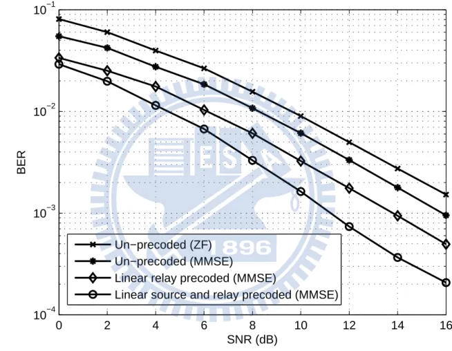
(a) an un-precoded system with ZF receiver, (b) an un-precoded system with MMSE receiver, (c) the optimal relay precoder with MMSE receiver [43], and (d) the linear source and relay precoded system. From those figures we can see that the linear source and relay precoded system outperforms not only the un-precoded system, but also the relay precoded system in [43]. This is because the linear source and relay precoded system incorporates the additional source precoder such that the performance can be enhanced even the direct link is not considered.

We also report the simulation result for cooperative beamforming, i.e., L = 1. As discussed in Theorem 2.1, our design for this case is optimal. We let N = R = M = 4 and SNRsr = 5

dB. Fig. 2.6 shows the BER comparison for the antennas selection method in [45] and the

linear source and relay precoded method. From the figure, we can see that the linear source and relay precoded method is superior to the antenna selection. This is expected since our design here is optimal.

§ 2.3.3 General MIMO Relay Channel

In this scenario, we consider a symmetric MIMO relay system, i.e., N = M = R = L = 4. As the previous case, each element of the channel matrices is assumed to be i.i.d. complex Gaussian random variables with zero mean and same variance. We let SNRsr, SNRrd be the

same as those defined in Section 2.3.2, and SNRsd as the SNR per receive antenna for the

(41)

Table 2.1: Complexity of linear source and relay precoders (MMSE receiver). Operation FLOPs

SVD, (2.14)-(2.16) (14MN2_{+ 8N}3_{) + (14RN}2_{+ 8N}3_{) + (14MR}2_{+ 8R}3₎

B−1_{, (2.24)} _2MN2_{+ 2MN + 2N}3 _{+ 13/4N}2_{+ N}2 ps,iand pr,i, (2.29)-(2.30) (21LIr+ 14LIs)Ii

˜

E, (2.33) 14L + 10M + 4NL + 2L2_N

SVD of ˜E, (2.34) 22L3

US, (2.35) 2L3

FSand FR, (2.20)-(2.21) (2NL + 2NL2) + (2R2+ 2R3)

N: number of transmit antennas R: number of relay antennas M: number of receive antennas

L: number of transmitted symbol streams Ir: number of iteration for computing pr,i

Is: number of iteration for computing ps,i

Ii: number of iteration of the water-filling process

2.7 and Fig. 2.8 show the MSE and BER comparisons, respectively, for the linear source and relay precoded system and other systems described in Section 2.3.2. Note that the optimal relay precoder in [43] only considers the two-hop relay system. For fair comparison, we include the direct link at the destination when implementing the MMSE receiver. As expected, the linear source and relay precoded method outperforms all other systems.

(42)

SR

H

#

Source: N antennas M M S E

#

Relay: R antennas Destination: M antennas SD

H

RD

H

: First phase : Second phase

F

S

s

y

R

F

R Nsubstreams

(43)

0 5 10 15 20 10−2 10−1 100 SNR (dB) MSE Un−precoded

Linear source and relay precoded

Figure 2.2: MSE performance comparison for un-precoded and linear source and relay precoded AF SISO-OFDM cooperative systems.

(44)

0 5 10 15 20 10−3 10−2 10−1 SNR (dB) BER Un−precoded

Figure 2.3: BER performance comparison for un-precoded and linear source and relay precoded AF SISO-OFDM cooperative systems.

(45)

0 5 10 15 20 25 10−1 100 SNR (dB) MSE Un−precoded (MMSE)

Linear relay precoded (MMSE)

Linear source and relay precoded (MMSE)

Figure 2.4: MSE performance comparison for existing un-precoded/precoded and linear source and relay precoded AF two-hop MIMO relay systems.

(46)

0 5 10 15 20 25 10−3 10−2 10−1 100 SNR (dB) BER Un−precoded (ZF) Un−precoded (MMSE)

Figure 2.5: BER performance comparison for existing un-precoded/precoded and linear source and relay precoded AF two-hop MIMO relay systems.

(47)

−2 −1 0 1 2 3 4 5 6 10−4 10−3 10−2 10−1 SNR (dB) BER Antenna selection

Figure 2.6: BER performance comparison for antenna selection [45] and linear source and relay precoded AF two-hop MIMO relay systems (L = 1 and N = R = M = 4).

(48)

0 2 4 6 8 10 12 14 16 10−1 SNR (dB) MSE Un−precoded (ZF) Un−precoded (MMSE)

Figure 2.7: MSE performance comparison for existing un-precoded/precoded and linear source and relay precoded AF MIMO relay systems.

(49)

0 2 4 6 8 10 12 14 16 10−4 10−3 10−2 10−1 SNR (dB) BER Un−precoded (ZF) Un−precoded (MMSE)

Figure 2.8: BER performance comparison for existing un-precoded/precoded and linear source and relay precoded AF MIMO relay systems.

(50)

(51)

Chapter 3 Joint MMSE Transceiver Design with

Tomlinson-Harashima Source and Linear

Relay Precoders

In this chapter, we address the problem of the MMSE transceiver design with a nonlinear THP. In Section 3.1, we first formulate the precoded system model in which a THP cascaded with a linear precoder are used at the source, a linear precoder at the relay, and the MMSE receiver at the destination. As that in the previous section, we found that the MSE is a complicated function of the source and the relay precoders, and the corresponding optimization is difficult to conduct. In Section 3.2, we then propose a new method to overcome the problem. The main idea is to use the primal decomposition such that the two-precoder design problem can be translated into a single-relay precoder problem. With the proposed method, the optimization problem can be further expressed as a convex optimization problem, and the closed-form solution can be obtained by KKT conditions. Finally, we evaluate the performance of the proposed method in Section 3.3.

(52)

§ 3.1 System Model and Problem Formulation

§ 3.1.1 MMSE Receiver with Tomlinson-Harashima Source and Linear Relay

Precoders

We consider the precoded three-node AF MIMO relay precoding system as shown in Fig. 3.1, where we include two precoders - a THP source precoder and a linear relay precoder FR, and a

linear MMSE receiver, G, is applied at the destination. Here, we also consider the general two-phase transmission protocol [41]- [45]. In the first two-phase, the source signal s ∈ CN ×1_{is fed into}

the nonlinear THP in which a successive cancellation operation characterized by a backward squared matrix B and a modulo operation MODm(·). The source signals s = [s1, · · · , sN]T are

modulated by m-QAM where the real and image parts of skas the set {±1, · · · , ±(

√

m − 1)}.

The feedback matrix B has a lower triangular structure and the diagonal elements are all zeros. The modulo operation acts over the real and image parts of the inputs, respectively, is expressed as follows: MODm(x) = x − 2 √ mbx + √ m 2√m c. (3.1)

It is clear that the transmitted signal x is bounded between −√m and √m. With B and the

operation in (3.1), the elements of x can be recursively expressed as [16]

xk= sk− k−1

X

l=1

B(k, l)xl+ ek (3.2)

where xk is the kth elements of vector x and B(k, l) is the (k, l) element of matrix B; e =

[e1, . . . , eN]T denotes the errors of the modulo operation (the difference of the input and the

output). From (3.2), we can reformulate the transmitted signal x after THP with the following matrix form

x = C−1_v _(3.3)

where C = B + IN is a lower triangular with ones in its diagonal, and v = s + e. The THP

合作式放大傳遞多輸入多輸出中繼系統之線性與非線性傳收機設計

國 立 交 通 大 學

電機工程學系

博 士 論 文

合作式放大傳遞多輸入多輸出中繼系統之

線性與非線性傳收機設計

Linear and Nonlinear Transceiver Designs in

Amplify-and-Forward MIMO Relay Systems

研 究 生：曾凡碩

指導教授：吳文榕

合作式放大傳遞多輸入多輸出中繼系統之線性與

非線性傳收機設計

Linear and Nonlinear Transceiver Designs in

Amplify-and-Forward MIMO Relay Systems

研究生：曾凡碩

Student:

Fan-Shuo

Tseng

指導教授：吳文榕 博士 Advisor:

Dr.

Wen-Rong

Wu

國立交通大學

電機工程學系

博士論文

A Dissertation

Submitted to Institute of Communication Engineering

College of Electrical Engineering

National Chiao Tung University

in Partial Fulfillment of the Requirements

for the Degree of Doctor of Philosophy

in

Electrical Engineering

Hsinchu, Taiwan

合作式放大傳遞多輸入多輸出中繼系統

之線性與非線性傳收機設計

研究生: 曾凡碩 指導教授: 吳文榕 博士

國立交通大學

電機工程學系博士班

摘要

Linear and Nonlinear Transceiver Designs

in Amplify-and-Forward MIMO Relay

Systems

Student: Fan-Shuo Tseng Advisor: Dr. Wen-Rong Wu

Institute of Communication Engineering

National Chiao Tung University

Abstract

Acknowledgements

Contents

List of Tables

List of Figures

Chapter 1

Introduction

D

Chapter 2

Joint MMSE Transceiver Design with

Linear Source and Relay Precoders

§ 2.1

System Model and Problem Formulation

§ 2.1.1

MMSE Receier with Linear Source and Relay Precoders

§ 2.1.2

MMSE Receiver and Related MSE Matrix

§ 2.1.3

Problem Formulation

§ 2.2

Joint Source/Relay Precoders Design

§ 2.2.1

Proposed Method

§ 2.2.2

Special Case: Cooperative Beamforming

§ 2.3

Applications

§ 2.3.1

SISO OFDM Relay System

§ 2.3.2

Two-Hop MIMO Relay System

§ 2.3.3

General MIMO Relay Channel

H

國立交通大學

博士論文

研究生：曾凡碩

指導教授：吳文榕博士 Advisor:

研究生: 曾凡碩指導教授: 吳文榕博士