時窗限制下的動態車輛路線問題之等待策略

行政院國家科學委員會專題研究計畫 成果報告

時窗限制下的動態車輛路線問題之等待策略

研究成果報告(精簡版)

計 畫 類 別 ： 個別型 計 畫 編 號 ： NSC 97-2221-E-009-119- 執 行 期 間 ： 97 年 08 月 01 日至 98 年 07 月 31 日 執 行 單 位 ： 國立交通大學運輸科技與管理學系（所） 計 畫 主 持 人 ： 黃家耀 報 告 附 件 ： 出席國際會議研究心得報告及發表論文 處 理 方 式 ： 本計畫可公開查詢

中 華 民 國 98 年 10 月 31 日

時窗限制下的動態車輛路線問題之等待策略

摘要 時窗限制下的車輛路線問題已經有廣泛的研究，問題主要為規劃車輛路線以滿足所有 含時間窗限制的需求點，而目標一般為最少車輛數與最少總行走距離。而近年由於電 子導航及通訊科技發展越趨成熟，幫助實時車輛指派與調度的可行性，而且得使在現 有路線上加入動態即時的需求變得可行。本研究之目的是要發展一套有效之等待策略 去求解動態的時窗限制下的車輛路線問題。等待策略意即把車輛安排在適當的地點等 待，使增加可以接受即時需求的可能性。透過幾何機率的方法，本研究發展出一套在 動態車輛路線問題可使用的最佳等待策略。 關鍵詞: 等待策略; 動態; 即時需求; 時窗限制下的車輛路線問題

Waiting Strategies for the Dynamic Vehicle Routing Problem with Time

Windows

Abstract

The Vehicle Routing Problem with Time Windows (VRPTW) is a well-known and classic problem in Logistic management and Operations research. The problem is to determine a set of routes for a fleet of vehicles visiting a number of known customers associated with time windows, and the objective is to minimize the number of vehicles required and the total travel time. The objective of this study is to develop an optimal strategy trying to maximize the probability of inserting new real-time requests in the existing route. This can be achieved by holding a vehicle at appropriate locations so as to exploit a larger region of service being able to reach at a limited slack time.

Some waiting strategies were proposed in a previous study (Yuen et al., 2009). In this study we developed a methodology to quantify the expected number of arrivals that a waiting strategy can insert. It is shown that the optimality of strategies should depend on more factors such as distances between locations, width to time windows and waiting times, and demand intensity.

Keyword: Waiting Strategies; Dynamic; Real-time request; Vehicle Routing Problem with Time Windows

INTRODUCTION AND BACKGROUND

The Vehicle Routing Problem with Time Windows (VRPTW) is a well-known and classic problem in Logistic management and Operations research. The problem is to determine a set of routes for a fleet of vehicles visiting a number of known customers associated with time windows, and the objective is to minimize the number of vehicles required and the total travel time. It is a combinatorial optimization problem and has been studied in numerous papers (see Cordeau et al, 2002). The dynamic vehicle routing with real-time requests has been becoming an important topic. In contrast to the static case in which known requests are preplanned before the day of operation, the dynamism of the problem are due to the time-dependent nature of the network travel time or real-time arrivals of customer requests, which are unknown beforehand. The characteristics of dynamic vehicle routing problems and early studies in this area were identified by Psaraftis (1995) and Gendreau and Potvin (1998).

In the dynamic problem, known requests with specified time windows are preplanned, while new customer requests are to be considered for possible insertion. A common approach to solve the problem for new customer arrivals are re-optimization. Re-optimization is a straight forward algorithm which repeats the static optimization algorithm each time the system is updated (e.g. on arrival of a new request) (see Gendreau et al., 1999). For the dynamic pickup and delivery problem with time windows, Mitrovic-Minic et al. (2004) proposed a double-horizon based heuristic which examine the benefit of updating frequency with short-term and long-term objectives.

Several recent papers contributed on the solution or computing methodology in increasing the demand acceptance rates, level of service, and/or reducing operating cost. Diana (2006) considered several characteristics of the information flow (including percentage of real-time requests, interval between call-in and requested pickup time, and length of the computational cycle time) in evaluating the effectiveness of how the input is revealed to the algorithm in dynamic. Coslovich et al. (2006) solved the routing of unexpected demands in the dial-a-ride problem, with a new two-phase insertion technique. In contrast, Branke et al. (2005) and Yuen et al. (2009) investigated the waiting strategies in the scheduling problem. In Yuen et al. (2009), a Modified Dynamic Wait (MDW) strategy was proposed to allocate the waiting times of a vehicle along the stops of a planned route, which can potentially increase the flexibility and reduce the operating cost in accepting future calls. Testing against the classic Drive First (DF) and Wait First (WF) strategies, MDW is shown to be superior in general. More robust algorithms and heuristics were developed by formulating the problem into shortest path problem (Fabri and Recht, 2006), artificial neural network (Fu, 1999) and fuzzy logic (Teodorovic and Radivojevic, 2000).

The above studies focused on the determination of customer sequence in routes. Another line of research to answer this question is to examine if it is possible to reduce the number of required vehicles and/or total distance travelled when a vehicle should wait at a location before moving to the next customers Yuen et al. (2009) investigated the dynamic dial-a-ride problem, and suggested a waiting strategy which holds a vehicle for possible future calls until the time (if no calls arrive) that it will arrive the next location and catch the earliest pickup time, in a just-in-time alike manner. It is shown to reduce the total distance by 5 to 7% in a simulation experiment.

More recently, Berbeglia et al. (2009) gave a review on the dynamic pickup and delivery problems and its variations. Some issues and recent new solution concepts are identified, such as vehicle diversion (Ichoua et al., 2000), degree of dynamism (Lund et al., 1996; Larson, 2000), anticipation of future requests (Ichoua et al., 2006; Tjokroamidjojo et al., 2006) with waiting and buffering strategy (Pureza and Laporte, 2008). For instance, a vehicle-waiting heuristics, which was proposed in Ichoua et al. (2006) for the dynamic vehicle routing and dispatching problem, investigated the value of knowledge of knowing the probabilistic arrivals of future demands. In their study, dummy customers are created representing forecasted requests, and the proposed strategy is used to decide for the vehicle to wait or not. Pureza and Laporte (2008) investigated a waiting strategy, which delays the assignment of vehicles to next destination, and a request buffering strategy, which postpones the assignment of non-urgent new requests to the next route planning. With numerical examples, it showed that request buffering improves the performances in the system with higher degree of dynamism.

MODEL FORMULATION AND SPECIFICATION

Vehicle trajectory

Three waiting strategies, namely, Drive First (DF), Wait first (WF) and Modified Dynamic Wait (MDW), were developed in Yuen et al. (2009) for the dynamic demand responsive transport services with time windows. Once the routes (i.e., the sequence of the stops) are determined, the allocation of waiting times at each stop can be calculated. The corresponding pseudo codes were given in Wong et al. (2009). In the VRPTW problem, given the time windows of each stop and the sequence of locations to visit, the vehicle trajectory by each of the strategies can be calculated with the procedure. In particular, Drive First and Wait First can be used as the earliest bound and latest bound of departure. Therefore, any trajectory above DF and below WF is feasible, and DF and WF forms the lower bound and upper bound of waiting at each location. As proposed in Wong et al. (2009), a Modified Dynamic Wait

(MDW) strategy suggests a feasible trajectory that can potentially saves number of vehicle and/or distance travelled.

The expected number of customer arrivals

The idea of the proposed dynamic waiting strategy tries to maximize the probability of accepting future calls. We would show and quantity this value in the following analysis. The probability of inserting an unknown request into an existing route can be analyzed with the method of geometric probability (see Larson and Odoni, 1981). For a case where a vehicle is moving from location i to i+1 after the service, with the travel time denoted as D and there is a slack time (i.e. waiting time) that enables the vehicle to detour and pickup a real-time request. As shown in Figure 1, if one adopts the DF strategy, the vehicle would spend the slack time at i+1, and therefore if it detours to a new customer from i+1 before the service can start, it has to move back to i+1 before moving on to i+1. The potential service region is a circle with the centre at location i+1, with a radius of S/2. On the other hand, with WF strategy, the vehicle would spend the slack time at i, and the service region is an ellipse, with locations i and i+1 as focal points, D as the distance between the two foci. Therefore the sum of distances from any point on the curve to the two foci is D+S.

Figure 1. Service Regions of Drive First and Wait First waiting strategies

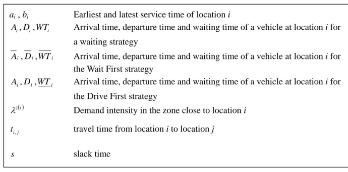
The size of the area implies how far a vehicle can go to pickup a new customer without violating the time windows planned requests. Then we can express the expected number of customers a vehicle can pickup based on a specific strategy. To facilitate the discussion, a list of the notations of variables and parameters are given in Table 1.

D = Direct travel time from location i to location j S = Slack time available for the vehicle to detour

(a) Service region for DF (b) Service region for WF

S/2 D i i+1 S/2 D i i+1

Table 1 Notations of input of customer requests

For the ellipse shown in Figure 2(a), it is easy to show that the semi-major axis is ⎟ ⎠ ⎞ ⎜ ⎝ ⎛ + 2 D S

and the semi-minor axis is _⎟⎟ ⎠ ⎞ ⎜ ⎜ ⎝ ⎛ + 2 4 2 SD S

, and the area is Ar

(

S,D

)

= _⎟⎟

⎠ ⎞ ⎜ ⎜ ⎝ ⎛ + ⎟ ⎠ ⎞ ⎜ ⎝ ⎛ + 2 4 2 2 SD S D S π .

The area is proportional to the possibility of accepting a new request at a particular time instance. As time goes by, the area covered is shrinking over time with the waiting, and the expected number of arrivals can be achieved by integrating the area, which is expressed as a function of waiting time.

Since [ai , bi] is the time windows of a location i, and [Di, A_i] is the latest feasible departure

time and earliest service time of a location i. Therefore, for any arbitrary waiting strategy, the following conditions should hold:

i i i A b

A ≤ ≤ ; a_i ≤D_i ≤Di

The expected number arrivals can be determined by the area covered multiplied by the duration of waiting and multiplied by the demand intensity.

Drive First strategy

The expected number arrival in the covered area at location i with the DF strategy, EA_iDF,

can be calculated by

(

_{D A t}

)

_λ ( )_{dω Ar}

(

_{D ω t}

)

_λ ( )_dω Ar EA D zi A i ii i z A WS A i i ii i i i i i

∫

∫

− + − = − , , DF , ,

ai , bi Earliest and latest service time of location i

i

A ,D ,_i WT _i Arrival time, departure time and waiting time of a vehicle at location i for a waiting strategy

i

A ,Di,WTi Arrival time, departure time and waiting time of a vehicle at location i for

the Wait First strategy

i

A ,D ,_i WT _i Arrival time, departure time and waiting time of a vehicle at location i for the Drive First strategy

( )i z

λ Demand intensity in the zone close to location i

j i

t, travel time from location i to location j

where the first term denotes the expected number of arrivals when the vehicle is on the way to location i, and the second term is the expected number of arrivals when the vehicle is waiting at location i. For more details, the first term is determined with the integration of the area covered with a slack

(

Di −A_i

)

during a period of WS before A , multiplied by _i λz( )i , the

demand intensity in the area (with the unit of number of arrivals per unit area per unit time). Here WS is a reasonable time width that a new request is considered by a route. Since the new request arrives when the vehicle is on the way to the location, the area covered is a fixed value over the integration. The second term is calculated by integrating the area from its arrival time

i

A to its departure time D . It can detour to a location and return with a before the latest _i

feasible departure time D . And the total expected number arrival with the DF strategy, i

DF EA , is calculated as

∑

= = n i i EA EA 0 DF DF .

Wait first strategy

The expected number arrival in the covered area at location i with the WF strategy, EA_iWF,

can be calculated by

(

_{A A t}

)

_λ ( )_{dω Ar}

(

_{A ω t}

)

_λ ( )_dω Ar EA D z i i A i ii i i z A WS A i i ii i i i i i 1 1 , 1 1 1 , 1 WF , , → + + ₊ → + − + +

∫

∫

− + − =

where the first term and second term, similar to the case of DF, denote the expected number of arrivals when the vehicle is on the way to location i and that when the vehicle is waiting at location i. The difference here is that the service is done once the vehicle arrives a location i, and therefore to pickup up a new request, say at location j, the vehicle can move from i to j to

i+1 without returning back to i. If a vehicle goes for a new request, it must return to i+1

before Ai+1. The demand intensity is considered for the region between i and i+1, and thus

approximated by ( ) ( ) ( ) ⎟ ⎟ ⎠ ⎞ ⎜ ⎜ ⎝ ⎛ ₊ = + + → 2 1 1 zi zi i i z λ λ

λ . And the total expected number arrival with the

WF strategy, EAWF, is calculated by

∑

= = n i i EA EA 0 WF WF .

Modified Dynamic Wait strategy

The case of modified dynamic wait can be determined in a similar way:

(

_{A A t}

)

_λ ( )_{dω Ar}

(

_{A ω t}

)

_λ ( )_dω Ar EA D z i i A i ii i i z A WS A i i ii i i i i i 1 1 , 1 1 1 , 1 MDW , , → + + ₊ → + − + +

∫

∫

− + − =

∑

= = n i i EA EA 0 MDW MDW

General Dynamic Wait strategy

The above cases have the properties that both A_i and D are earlier than or equal to _i a _i

(for DF) in which any detour must return to location i, or both A_i and D are later than or _i

equal to a (for WF and MDW) in which any detour must not return to location i. For a _i

general dynamic waiting strategy, it could happen that A_i <a_i <D_i, and the area covered would be different if a request arrive before the earliest service time a or after _i a . _i

(

)

( )

(

)

( )

(

)

( )

(

)

( )

(

)

( ) i i i i z D A i ii i i z A WS A i i ii i i i i z D a i ii i z a A i ii i z A WS A i i ii i a A if d t A Ar d t A A Ar a A if d t A Ar d t D Ar d t A D Ar EA i i i i i i i i i i > − + − ≤ − + − + − = + → + + + → − + + + → + + −

∫

∫

∫

∫

∫

, , , , , 1 1 , 1 1 1 , 1 1 1 , 1 , , GDW ω λ ω ω λ ω λ ω ω λ ω ω λ

∑

= = n i i EA EA 0 GDW GDW

The above equations measure the ability to insert an additional customer. The above example only shows the idea with two stops and no subsequence customers after i+1, and therefore it seems WF is more attractive than DF with its larger service area covered. As shown in Yuen et al. (2009), it is only true when there are not many demands. The actual calculation will be more complicated if we consider more than 2 stops and take the time windows into consideration. One reason is that D is sometimes constrained by i b_i+1 or b_i+2 but not b . _i

For a route with several stops, there is a slack for each of the stops because of the time windows. This slack may be reserved to the subsequence stops if the length of the time window of the next stop is wide enough. If this slack cannot be reserved because of the narrow time window of the next stop, the value of the slack is zero. With the Drive First and Wait First strategies which can determine the lower and upper envelopes of waiting at a particular location, we can analyze the maximum serve region of detouring to pickup a future request based on the distance between the stops and the slack times.

NUMERICAL EXPERIMENTALS

With the above derived equations, it can be proved that there is no single waiting strategies dominate in all situations. We show that in a numerical experiment with three scenarios: tight schedule, loose schedule, and loose schedule with scatter demand locations. The results are shown in Table 2 with demand intensity set to be 0.01 across the whole study area.

Under a tight schedule, with WF it has a higher chance of inserting a new request than with DF. MDW and GDW are identical to WF, which is optimal in this case. For the case of loose schedule, DF is some what better than WF, but it can be significant improved with the proposed MDW. However, MDW, with W(MDW)={0.5, 4, 2, 5, 1, 0}, is not an optimal strategy in this scenario, as one can use a general waiting time strategy and allocate the waiting time from location 0 to location 1, such that and W(GDW)= {0, 4.5, 2, 5, 1, 0}. Looking into the details of the calculation, it is because of the short distance between 0 and 1 (t_0,1=0.5) and the large value of D (with 1 Di−A_i = 7-0.5 = 6.5). Therefore, spending a

waiting time at location 0 can make a very small benefit with the detour, but there is a larger service radius with waiting at location 1.

The third scenario shows a loose schedule with cluster locations, in which we modified the scenario 2 with the distances between locations to be 1 time unit. It models the situation of cluster locations, as compared to the time window width of 2 time unit. In this case, DF is superior to WF and MDW. It is a surprising finding, as previous studies demonstrated that MDW should be better than DF. However, one would argue that the measuring criteria used here, i.e. expected arrivals (EA), and may not be useful if the routes are quite empty. It would then be interested to know the opportunity cost of inserting a new request, i.e. the reduction of EA. If a new feasible call arrives, what is the probability of taking another call if the current new request is rejected (or inserted to another route)? This is worth further investigation. Furthermore in the example, it is showed that a GDW can be derived that is superior to DF and MDW. It reemphasizes that the optimality of a waiting strategy should also take into account the clustering of request locations, total length of waiting times (tightness of schedule), and demand intensity.

CONCLUSIONS AND SELF EVALUATION

In this research we have establish a methodology to quantify the performance of a waiting strategy for the dynamic vehicle routing problem with time windows. It is found that the optimality of a waiting strategy should depend on clustering of request locations and tightness of the schedule, and therefore the previous proposed strategy derived from only the time windows and sequence of locations may not be optimal. This research opened an avenue to look at the problem of waiting strategies with geometric probability rather than simulation. To derive an exact optimal strategy, it is worth to further investigate the opportunity cost of inserting a new request and also the probability of taking another call if the current new request is rejected.

0 5 10 15 20 25 0 1 2 3 4 5 6 Locations Tim e [ai bi] DF WF MDW GDW

Figure 1. Trajectories of a vehicle using the three waiting strategies (Scenario 3)

Table 2. Allocation of waiting times in different scenarios

Locations (i) 0 1 2 3 4 5 Scenario 1: A tight schedule ai 0 1 3 5 10 15 bi 0 3 5 7 10 15 t(i,i+1) 0.5 3 3 3 3 Wi (DF) 0 0.5 0 0 0 2 EA (DF) 0.0219 Wi (WF) 0.5 0 0 0 2 0 EA (WF) 0.7184 Wi (MDW) 0.5 0 0 0 2 0 EA (MDW) 0.7184 Wi (GDW) 0.5 0 0 0 2 0 EA(G DW) 0.7184 Scenario 2: A loose schedule

ai 0 1 7 11 18 21 bi 0 3 9 13 18 21 t(i,i+1) 0.5 2 2 2 2 Wi (DF) 0 0.5 4 2 5 1 EA (DF) 2.4781 Wi (WF) 2.5 4 2 3 1 0 EA (WF) 2.4187 Wi (MDW) 0.5 4 2 5 1 0 EA (MDW) 4.5972 Wi (GDW) 0 4.5 2 5 1 0 EA(G DW) 4.7096 Scenario 3: A loose schedule with c luster locations

ai 0 1 7 11 18 21 bi 0 3 9 13 18 21 t(i,i+1) 0.5 1 1 1 1 Wi (DF) 0 0.5 5 3 6 2 EA (DF) 5.2051 Wi (WF) 2.5 5 3 4 2 0 EA (WF) 1.936 Wi (MDW) 0.5 5 3 6 2 0 EA (MDW) 3.9321 Wi (GDW) 0 0.5 5 3 8 0 EA(G DW) 5.3247

References

Berbeglia, G., Cordeau,J.F. and Laporte, G., 2009. Invited review: Dynamic pickup and delivery problems. European Journal of Operational Research. In press.

Branke, J., Middendorf, M., Noeth, G. and Dessouky, M., (2005) Waiting strategies for dynamic vehicle routing. Transportation Science, 39, 298–312.

Cordeau, J.-F., Desaulniers, G., Desrosiers, J., Solomon, M.M., Soumis, F. (2002) VRP with time windows. In P. Toth and D. Vigo (eds.): The vehicle routing problem, SIAM monographs on discrete mathematics and applications, Vol. 9, Philadelphia, 157-193.

Coslovich, L., Pesenti, R., Ukovich, W., 2006. A two-phase insertion technique of unexpected customers for a dynamic dial-a-ride problem. European Journal of Operational

Research 175, 1605 – 1615.

Diana, M., 2006. The importance of information flows temporal attributes for the efficient scheduling of dynamic demand responsive transport services, Journal of Advanced

Transportation 40, 23-46.

Fabri, A., Recht, P., 2006. On dynamic pickup and delivery vehicle routing with several time windows and waiting times, Transportation Research part B 40, 335-350.

Fu, L., 1999. On-line and off-line routing and scheduling of dial-a-ride paratransit vehicles,

Computer-aided Civil and Infrastructure Engineering 14, 309-319.

Gendreau, M., F. Guertin, J.-Y. Potvin, E. Taillard. (1999) Parallel tabu search for real-time vehicle routing and dispatching. Transportation Science, 33, 381–390.

Gendreau, M., Potvin, J.-Y. (1998) Dynamic vehicle routing and dispatching. In Fleet

Management and Logistics (T. Crainic, G. Laporte, eds.). Kluwer, London, UK,

115–126.

Ichoua, S, M. Gendreau and J-Y. Potvin (2000) Diversion issues in real-time vehicle dispatching. Transportation Science, 34, 426-438.

Ichoua, S., Gendreau, M., Potvin, J.-Y., 2006. Exploiting knowledge about future demands for real-time vehicle dispatching. Transportation Science 40, 211–225.

Larsen, A., 2000. The dynamic routing problem. Ph. D. dissertation, Technical University of Denmark, Kongens, Lyngby, Denmark.

Larson, R.C. and Odoni, A.R. (1981) Urban Operations Research, Prentice-Hall.

Mitrovic-Minic, S., Krishnamurti, R. and Laporte, G., (2004) Double-horizon based heuristics for the dynamic pickup and delivery problem with time windows. Transportation

Research Part B, 38, 669 – 685.

Psaraftis, H.N. (1995) Dynamic vehicle routing: Status and prospects. Annals of Operations Research, 61, 143–164.

Pureza, V., Laporte, G., 2008. Waiting and buffering strategies for the dynamic pickup and delivery problem with time windows. INFOR 46, 165–175.

Teodorovic, D., Radivojevic, G., 2000. A fuzzy logic approach to dynamic dial-a-ride problem,

Fuzzy Sets and Systems 116, 23-33.

Tjokroamidjojo, D., Kutanoglu, E., Taylor, G.D., 2006. Quantifying the value of advance load information in truckload trucking. Transportation Research part E 42, 340–357.

Wong, K.I., Yuen, C.W. and Han, Anthony F. (2009) On Dynamic Demand Responsive Transport Services with Degree of Dynamism. (Submitted)

Yuen, C.W., Wong, K.I. and Han, Anthony F. (2009) Waiting strategies for the dynamic dial-a-ride problem. International Journal of Environment and Sustainable

出席國際學術會議心得報告

計畫編號 NSC 97-2221-E-009-119 計畫名稱 時窗限制下的動態車輛路線問題之等待策略 出國人員姓名 服務機關及職稱 黃家耀 助理教授, 國立交通大學, 運輸科技與管理學系 會議時間地點 20-22 July 2009, Hong Kong

會議名稱 The Eleventh International Conference on Advanced Systems for Public

Transport (CASPT)

發表論文題目 Reliability-based stochastic transit assignment with capacity constraints

With the sponsorship of the National Science Council, I have attended the Eleventh

International Conference on Advanced Systems for Public Transport (CASPT) this year. The

main focus of the conference is to serve as a forum for the researchers and practitioners to discuss on the public transport planning and operations. The paper was presented in the conference, and I was also asked to chair a session.

A copy of the abstract is attached for reference.

Publication:

1. Szeto, W.Y., Solayappan, Muthu and Wong, K.I. (2009) Reliability-based stochastic transit assignment with capacity constraints. In Proceedings of the Eleventh International

RELIABILITY-BASED STOCHASTIC TRANSIT ASSIGNMENT WITH CAPACITY CONSTRAINTS

W.Y. SZETOa, Muthu SOLAYAPPANb, K. I. WONGc

a

Department of Civil Engineering, National University of Singapore, 1, Engineering Drive 2, Singapore 117576, Fax: +65-67791635, E-mail: [email protected]

b

Department of Civil Engineering, National University of Singapore, 1, Engineering Drive 2, Singapore 117576, Fax: +65-67791635, E-mail: [email protected]

c

Department of Transportation Technology & Management, National Chiao Tung University, 1001 Ta Hsueh Road, Hsinchu, 30010, TAIWAN, Fax: +886-(0)3-5720844,

E-mail: [email protected]

ABSTRACT

This paper proposes a Linear Complementarity Problem (LCP) formulation for risk-taking stochastic transit assignment problem with capacity constraints. A route-based linear programming (LP) reformulation of the LCP formulation is also proposed. A new solution method based on the column generation technique is developed to solve the proposed LP. The solution method utilizes the k-shortest path algorithm, revised simplex method and sorting algorithm to solve the LP and guarantees finite convergence. Numerical results are reported for an example transit network based on Singapore’s bus network. Based on the results obtained, the proposed approach is also compared with the congestion cost function approach implicitly capturing stochastic capacity. Sensitivity analysis of parameters involved is also discussed in detail.