網路控制系統之時間延遲補償設計

(1)

國

立

交

通

大

學

電控工程研究所

博

士

論

文

網路控制系統之時間延遲補償設計

Networked Control Systems Design with the

Time Delay Compensation

研究生：賴建良

(2)

網路控制系統之時間延遲補償設計

研究生

:

賴建良指導教授

:

徐保羅博士

國立交通大學

電控工程研究所

摘要

近年來隨著網路的興起，即時的網路控制成為一種趨勢，在工業上的應用也越來越多，其可以很便利達成系統性的維護。然而，將控制系統網路化之後，也帶來了幾個缺點，例如：在共享的有限網路資源，隨著使用者數目的增減而造成變化極大的時間延遲，此問題輕則明顯降低系統效能，重則使整個系統產生不穩定的情形。根據網路協定、節點數和軟硬體條件，網路的時間延遲特性可能是固定或是有界的，甚至是隨機和不可預測的。因此，針對處理實際網路的重大的時間延遲變化，本論文提出兩種網路控制系統(NCS)之時間延遲補償的方法。第一個方法是發展即時的時間延遲估測，透過量測實際網路環境中兩個節點封包往返的時間(RTT)，可估測網路控制系統的時間延遲，並應用於三個方面：（1）發展適應性史密斯預估控制，可針對重大的時間延遲變化作處理；（2）強健性的網路控制系統設計，可對付具有局部時間延遲變化與外部干擾的 NCS；及（3）多重取樣週期的設計，可針對無線網路的壅塞問題作解決。上述所提之方法均已成功地實現於一交流伺服馬達的遠端控制系統。此外，第二個解決時間延遲的方法，是提出時間延遲完全補償策略(PDC)，能有效處理網路所引起時間延遲的影響，既不需要系統的模型也不用已知時間

(3)

延遲的資訊。網路控制系統能等效為原來的閉迴路系統串接一單純的時間延遲。因此，當引用 PDC 在設計網路控制系統時，不需考慮對網路時間延遲的影響，只需將所設計的控制系統直接實現於網路上即可。最後，實驗結果透過十五公里的 Internet 網路連線，進一步證明 SISO 和 MIMO 控制系統，都可經由所提出的 PDC 直接施行網路化，在實際網路環境保持其系統閉迴路的特性。

關鍵詞：網路控制系統、網路時間延遲、即時時間延遲估測、多重取樣週期的設計、時間延遲完全補償、網路化

(4)

Networked Control Systems Design with the

Time Delay Compensation

Student : Chien-Liang Lai Advisor : Dr. Pau-Lo Hsu

Institute of Electrical and Control Engineering

National Chiao Tung University

ABSTRACT

Real-time network control applications have increasingly gained attentions due to the rapid development of data communication network technologies. Network systems can be conveniently and systematically maintained in industrial applications. The networked control system (NCS), which simply interconnects all sensors, actuators, and controllers through the network, is promising in the future development of industrial technologies with low integration cost. However, NCS also leads to unavoidable problems in time delays that seriously degrade control performance and stability. The characteristics of network-induced delays may be in constant, bounded, random, or unpredictable natures depending on the network protocols, nodes, software, and hardware. In this study, there are two approaches proposed for NCS design under significantly varied time delays. In the first approach, on-line estimation of the delay time is developed by processing the on-line measurement of the round-trip time (RTT) between two nodes in real network environments. Three related controllers are thus developed: (1) the adaptive Smith predictor control scheme for significantly varied time delay, (2) the robust NCS design for bounded variation of time delay and disturbance, and (3) the multi-rate design under the condition of wireless network congestion.

The second approach is proposed as the model-free perfect delay compensation (PDC) scheme. This scheme effectively deals with network-induced delays requiring

(5)

neither the delay time information nor the plant model. NCS with PDC is thus simply equivalent to the original closed-loop system with an additional pure time delay and it is designed without concerning the network. Therefore, the well-designed controller can be directly implemented on a network and its stability can be guaranteed without being affected by the varied time delay. The proposed approaches have been successfully applied to remote control systems under significantly time-varying delay to control an AC servo motor. Provided experimental results have further proven that both SISO and MIMO systems can be directly implemented in networking systems by including the proposed PDC to maintain its original feedback-loop characteristics.

Keywords: Networked control system (NCS), network-induced delay, on-line delay estimation, multi-rate sampling, perfect delay compensation (PDC), MIMO NCS, direct networking

(6)

Acknowledgment

本論文得以順利完成，首先要感謝指導教授徐保羅博士在課業與研究上孜孜不倦的教誨，以及為人處事和靈性的啟迪，使我獲益良多，在此由衷地表達我最誠摯的敬意與感謝；同時，還要感謝王伯群教授的協同指導，於研究上適時的建議與鼓勵，其溫文儒雅的學者風範，更是我學習的標竿。此外，也要感謝口試委員：鄧清政教授、林志民教授、蔡清池教授、連豊力教授及蕭得聖教授等師長於百忙之中撥冗審閱，斧正本論文，使其更加周延與完整。論文進行期間，還要感謝實驗室的學長與學弟們，在生活及研究上的相互幫助及砥礪。在這段時光中，隨著女兒的出生，有了特別的經歷，如半夜將襁褓中女兒放在胸前趕作業、女兒稍大淘氣地將程式多加幾個字母，讓程式編譯產生錯誤…等等，領受初為人父的酸甜苦辣，對生命也產生不同的看法。同時，也經歷有學弟求學過程中因病去世，也有人服役、就業及結婚，邁向人生不同的階段，藉由彼此生命中的交集，學習成長。由於曾經一起同甘共苦生活過的學長學弟們，人數眾多無法一一列舉，只能由衷地感激，感謝你們在這段期間帶給我最珍貴的回憶。此外，還要謝謝慧霖於事務上的協助。最後，謹將此論文獻給我最敬愛的父親賴華龍先生與母親范玉妹女士及家人，感謝你們使我得以在無虞的環境中專心求學，同時還要感謝妻子嬿瑜及其家人的支持與關心，更要謝謝可愛女兒育萱的貼心陪伴。因為有了大家的支持與關懷，我才能夠無後顧之憂，完成學位。再次地感謝求學過程中所有曾經幫助過我和默默祝福我的師長及朋友們，謝謝您們。

(7)

List of Figures

Fig. 2.1 The NCS block diagram ... 11 Fig. 2.2 The experimental setup ... 11 Fig. 2.3 The package transition diagram ... 12 Fig. 2.4 Measured Internet delays (a) NCTU Lab<->NCTU Lab and

(b) NCTU Lab<-> Hukuo ... 14 Fig. 2.5 The simplified block diagram of NCS ... 15 Fig. 2.6 The system with the Smith predictor (a) the original system and

(b) the equivalent system. ... 15 Fig. 2.7 The block diagram of the adaptive Smith predictor with a PI controller ... 16 Fig. 2.8 The CAN data frame in the proposed NCS for measuring RTT ... 17 Fig. 2.9 The illustrative example for the time-delay estimation: (a) the architecture of

the proposed RTT measurement, and (b) the four transmitted models for the RTT and the time delay estimation. ... 19 Fig. 2.10 The control structure with the adaptive Smith predictor ... 20 Fig. 2.11Experimental results for system identification ... 21 Fig. 2.12 Simulation results for (a) the PI controller, (b) the Smith predictor (tm=200 ms)

with PI controller, and (c) the adaptive Smith predictor with PI controller. ... 22 Fig. 2.13 Experimental results on Intranet (a) PI controller, (b) Smith predictor

(tm =5 ms), and (c) adaptive Smith predictor. ... 23

Fig. 2.14 Experimental results on Internet (15 Km) (a) PI controller, (b) Smith predictor (tm= 46 ms), and (c) adaptive Smith predictor. ... 24

Fig. 2.15 Experimental results for the adaptive Smith predictor (without the initial delay). .... 25 Fig. 2.16 Experimental results for the adaptive Smith predictor (with the initial delay). ... 25 Fig. 3.1 Measured time delay ... 28

(11)

Fig. 3.2 The time delay effect measured RTT at (a) 9:00 am, and (b) 12:00 pm ... 29

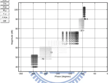
Fig. 3.3 Plant templates at certain frequencies ... 32

Fig. 3.4 Frequency responses with parameter variation ... 32

Fig. 3.5 The control structure with the adaptive Smith predictor ... 33

Fig. 3.6 The equivalent system by applying the Smith predictor ... 33

Fig. 3.7 Simulation sinusoidal responses of NCS for (a) PI controller, (b) PI + Smith predictor, and (c) PI + adaptive Smith predictor ... 35

Fig. 3.8 Responses of (a) PI and (b) QFT, both utilizing the adaptive Smith predictor (with 1J payload variation) ... 36

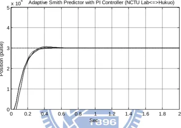
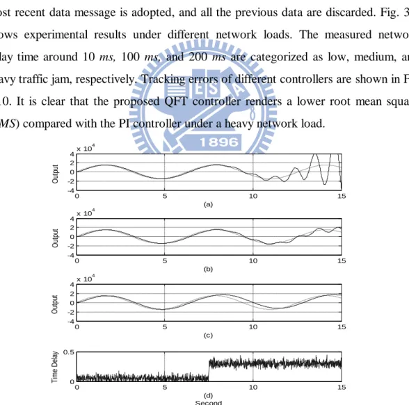
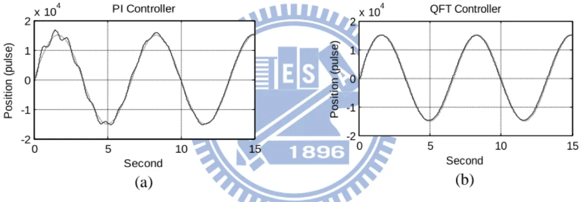
Fig. 3.9 Experimental results of the different controllers in heavy traffic load for (a) PI and (b) QFT ... 36

Fig. 3.10 Tracking errors of the different controllers in a high traffic load for (a) PI and (b) QFT ... 36

Fig. 3.11Tracking errors with the adaptive Smith predictor under the external disturbance (1J) in high traffic load with (a) PI and (b) QFT ... 37

Fig. 4.1 The block diagram of HNCS ... 40

Fig. 4.2 Experimental setup (a) experimental platform, (b) diagram of HNCS, and (c) the HNCS block diagram ... 41

Fig. 4.3 The diagram block of the gateway between wireless 802.11g and CAN ... 42

Fig. 4.4 The package transmission diagram ... 43

Fig. 4.5 Measurement of the delay time on CAN network (a) transmit time for a node-to-node and (b) the RTT between the gateway and the client ... 44

Fig. 4.6 Measurements of time delay in (a) a simple environment and (b) a complex environment... 45

(12)

Fig. 4.8 The HNCS performance with the bounded time-delay effect (1 s ~ 4.5 s) and

the unbounded time-delay effect (after 4.5 s) ... 47

Fig. 4.9 Nyquist plots with different time delay ... 48

Fig. 4.10 Structure of the multi-rate design method. ... 48

Fig. 4.11The frame of the CAN network in the proposed HNCS. ... 49

Fig. 4.12 Experimental results (a) the measured time delay and (b) the of switching the sampling time. ... 50

Fig. 4.13 The total switching times versus the window length. ... 52

Fig. 4.14 The responses of estimation results applying the median filter (window length N=5) ... 52

Fig. 4.15 The control structure of NCS with the adaptive Smith predictor ... 52

Fig. 4.16 Experimental results with the switching sampling time. ... 54

Fig. 4.17 Experimental results with a Smith Predictor and the switching sampling time. ... 55

Fig. 4.18 Experimental results with an adaptive Smith Predictor and the switching sampling time ... 55

Fig. 5.1 Block diagram of the general NCS ... 59

Fig. 5.2 The NCS with the adaptive Smith predictor... 60

Fig. 5.3 The block diagram of CDOB ... 62

Fig. 5.4 NCS with scattering transformation ... 63

Fig. 5.5 The scattering transformation ... 63

Fig. 5.6 (a) Butterfly element, (b) modified anti-butterfly element, and (c) modified butterfly element ... 65

Fig. 5.7 The control structure with PDC in the proposed NCS ... 65

(13)

Fig. 5.9 Simulation results of the NCS for (a) constant time delay (RTT = 400 ms)

with (b) scattering transformation and (c) PDC ... 69

Fig. 5.10(a) Time-varying delay, (b) NCS with scattering transformation, and (c) NCS with PDC. ... 70

Fig. 5.11The time-delay measurement in (a) Intranet and (b) Internet ... 72

Fig. 5.12Output response of the proposed NCS without PDC for a small time delay in Intranet ... 73

Fig. 5.13NCS without PDC for a large but constant time delay ... 73

Fig. 5.14NCS with PDC for a large but constant time delay ... 73

Fig. 5.15NCS with PDC in a varied time delay ... 74

Fig. 5.16Experimental platform with an 18 cm flexible beam driven ... 75

Fig. 5.17 (a) The Bode diagram of the flexible system, (b) the time response without vibration suppression, and (c) the time response with the notch filter. ... 76

Fig. 6.1 Block diagram of the general MIMO NCS………. 81

Fig. 6.2 The block diagram of the packet-based MIMO NCS………... 82

Fig. 6.3 (a) The control structure with PDC in the MIMO NCS and (b) Equivalent of the block diagram for MIMO NCS……… 83

Fig. 6.4 Step response without the network……….. 85

Fig. 6.5 Simulation results without PDC (a) RTT = 80 ms and (b) RTT = 120 ms………… 86

Fig. 6.6 Simulation result with PDC for the constant RTT = 120 ms……… 87

Fig. 6.7 Experimental setup………... 87

Fig. 6.8 Experimental results without PDC under a minor delay (varied from 6 to 52 ms, average 15.91 ms)……… 89

Fig. 6.9 Experimental results with PDC under a minor delay (varied from 14 to 107 ms, average 19.51 ms)……… 89

(14)

Fig. 6.10 Experimental results without PDC under a major delay (varied from 141 to 412 ms, average 219.17 ms)………..90 Fig. 6.11 Experimental results with PDC under a major delay (varied from 210

(15)

List of Tables

Table 1.1 Classification of current approached in NCS control design ... 3

Table 3.1 The averaged delay time for the Ethernet and CAN networks ... 29

Table 3.2 Comparison of tracking performance (without external disturbance) ... 37

Table 3.3 Comparison of tracking performance (with external disturbance) ... 38

Table 4.1 The averaged delay time of the hybrid networks in a simple environment (unit: ms） ... 45

Table 4.2 The averaged delay time of the hybrid networks in a complex environment (unit: ms ) ... 45

Table 4.3 The averaged delay time by switching the sampling time ... 51

Table 5.1 Comparison of control performance under different methods... 69

Table 5.2 Comparison of the four NCS approaches ... 71

(16)

Chapter 1 Introduction

Real-time network control applications are increasingly gaining attentions on account of the rapid development of network technologies with data communication through the Internet. Networked control systems (NCS) have become more popular because they can be easily maintained in industrial applications with a convenient and systematic manner. Their future applications are promising, encompassing a spectrum as wide as in space exploration, hazardous environments, factory automation, remote diagnostics and troubleshooting, remote mobile robots, aircraft, automobiles, manufacturing plant monitoring, nursing homes, and tele-operations, etc. However, network-induced time delay is unavoidable in NCS, and stability is still highly concerned in NCS design. Moreover, as the number of nodes increases when all sensors, actuators, and controllers are interconnected within a network, real-time NCS performance is seriously degraded by the time delay effect and becomes unstable due to the limited network bandwidth. Therefore, controllers obtained from general design without considering the network are not suitable for NCS implementation and have to be redesigned or modified to minimize the time delay effect which mainly causes the time delay and data dropout.

1.1 General review

Many researchers have been working on NCS during the past decades. The effect of integrated communication and control problems were discussed by Halevi and Ray (1988) and Liou and Ray (1991). Recent research topics and challenges in NCS have attracted attentions mainly on (1) control of networks in the protocol, (2) control over networks in the application layer, and (3) multi-agent systems (Tatikonda and Mitter, 2004; Baillieul and Antsaklis, 2007; Hespanha et al., 2007; Zampieri, 2008; Gupta and Chow, 2010). The main issues regarding NCS design can be categorized into two types: (a) the time delay and (b) the data dropout. Transmission control protocol (TCP) is a reliable stream delivery service that it guarantees transmission of a data stream sent

(17)

from one node to another node without duplication or data loss but TCP also plays the major role of network-induced delays.

NCS performance will be degraded if a lower sampling rate is adopted owing to the limited network bandwidth. On the other hand, a faster sampling rate is more desirable in the sampled-data system to improve its performance. However, it also increases the network load, which it in turn results in a longer transmission delay. Thus, finding a suitable sampling rate to tolerate the network-induced delay and to achieve desirable system performances are crucial in NCS design. Lian et al. (2002) identified several key components of the time delay in order to determine an acceptable working range of sampling periods for NCS design.

On the other hand, some approaches have been proposed to improve communication protocols and eliminate competition for the shared network medium. Although some approaches allow each node on the network to transmit and receive data according to a predetermined schedule, for example, redesigning the protocols enhances transmission technology and provides guaranteed quality of service (QoS)for real-time requirements (Soucek and Sauter, 2004; Grenier and Navet, 2008), consumers can only access network resources in the application layer of the open system interconnection (OSI) model, and these protocols are not easily modified according to users’ requirements to improve NCS performance in real applications.

Recent research about the time delay of NCS mainly focused on modeling, stability, and controller design. In modeling techniques, some methodologies have been developed such as the Markov chain (Nilsson, 1998), probability distribution (Lian et al., 2002), a communication model for TCP (Chen et al., 2007), and the Takagi–Sugeno (T–S) model in network-induced delays (Zhang et al., 2007). In stability analysis, a necessary and sufficient condition ensuring a stable NCS was presented with random delays in less than one sampling period only (Yue et al., 2004; Zhang et al., 2005; Dritsas and Tzes, 2009). An asymptotically stable problem with a certain time-bound varying delay is solved by using Lyapunov functions (Zhang et al., 2001; Zhivoglyadov and Middleton, 2003). The maximum allowable delay bound (MADB) was proposed for NCS stability analysis (Kim et al., 2003). Basically, the

(18)

induced network delay varies according to the network load, the scheduling policy, the number of nodes, and the different protocols. The network-induced time delay with time-varying characteristics makes modeling and stability analysis for NCS more difficult. Thus, studies in network delays mainly for the controller design are crucial in NCS design.

1.2 Model-based NCS control design

Many NCS controller design methods have been proposed to deal with network-induced delays. Most available approaches are based on the model-based design to alleviate the network time delay effect. Available approaches can be categorized as shown in Table 1.1. Among these NCS control design methods, only two methods are designed without information of the time delay. Classification of major approaches in NCS control design and details are discussed below.

Table 1.1 Classification of major approaches in NCS control design

Model-based NCS design

Time Delay Constraint Methods

Known delay

Constant delay time 1. Smith predictor (Peng et al., 2004) Time-varying delay <

sampling time

1. State feedback controller

(Tang et al., 2008) 2. H robust controller

(Gao and Chen, 2008)

Bounded time-varying delay > sampling time

1. Model predictor control (Zhao et al., 2009)

2. Gain scheduler middleware (Tipsuwan and Chow, 2004) 3. Switched system approach

(Xie et al., 2008) 4. Fuzzy controller (Lee et al., 2003) 5. Optimal controller (Li et al., 2009) Unknown delay Constant 1. CDOB

(Natori and Ohnishi, 2008) 2. Scattering transformation

(Matiakis et al., 2009) Time-varying delay 1. CDOB

(19)

(1) The known network-induced delay

The popular time delay compensation scheme, known as the Smith predictor, was also proposed to deal with a constant delay time for NCS (Peng et al., 2004). Robust control and state feedback are achieved with the general assumption that the varied delay is relatively small compared with its sampling time (Gao and Chen, 2008; Tang et al., 2008). If the delay is longer than one sampling period, it may result in difficulties in dealing with vacant sampling and message rejection in the real-time NCS. Thus, robust NCS design results are only suitable for NCS with a small time-varying delay only.

Different techniques for the bounded-delay cases were proposed such as predictive control, switched system, optimal design, and gain scheduler middleware (Zhao et al., 2009; Xie et al., 2008; Li et al., 2009; Tipsuwan and Chow, 2004). Model predictor control (MPC) was also proposed with a sequence of control signals to be sent to compensate for irregular communication error with a known limitation of time delay (Yang, 2007; Zhao et al., 2009). The switched system was proposed to study asymptotical stability for a large system with a known time delay model (Zhai et al., 2002; Xie et al., 2008). For estimating the distribution of time delay, the algorithm of the optimal stabilizing gain was used (Li et al., 2009). In real NCS implementation over the Internet, the time delay which usually varies depending on the number of user nodes and communication data loads is relatively large compared with the sampling time. Thus, the design and implementation of NCS become more complicated in real applications.

Tipsuwan and Chow (2004) proposed the use of a gain scheduler middleware (GSM) to adjust the NCS controller gain, maintain control performance, and stabilize the system with respect to the real-time network traffic conditions with the measured probing packet RTT. The GSM design adopting a known upper-bounded delay also avoids the high gain controller as well as the input saturation. However, most of the abovementioned research results are limited to the time delays in constant, less time-varying, or bounded natures, which are not true in real network environments. The time delay induced during the transmission over the communication network becomes more unpredictable because the network time delay significantly varies due to

(20)

the varied loads, scheduling, number of nodes, and protocols. The NCS design results generally obtained from a nominal model with a known delay time thus become invalid for real NCS applications.

(2) The unknown network-induced delay

Recently, the communication disturbance observer (CDOB) (Natori and Ohnishi, 2008) and the scattering transformation with a known system model (Matiakis et al., 2009) have been proposed to effectively compensate for unknown constant time delays in NCS. Although CDOB can be extensively applied to conditions with the time-varying delay, and undesirable performance with oscillation and noise are still present in the CDOB output in practice. On the other hand, the scattering transformation with a known system model is also not applicable to real NCS with varied time delays (Matiakis et al., 2009). Moreover, these newly developed NCS design approaches still require an accurate system model in the design procedure.

Network-induced time delays may be constant, bounded, stochastic, random, or unpredictable depending on the network protocol and hardware. Therefore, network-induced delays have different natures especially in a shared Internet with a huge number of network users at the same time. Although some methods have been proposed to eliminate the time delay effect from its closed control loop in NCS design, the design results obtained are usually based on a system model with known and bounded delay information. Therefore, those model-based methodologies are usually not applicable to real networks with significantly varied time delays.

1.3 Problem statement

Although many methods have been proposed to design controllers for NCS with network-induced delays in the past two decades, some critical issues still exist as follows:

(1) Network-induced delay is unpredictable, especially in a shared Internet with a huge number of user nodes.

(2) Network time delay significantly varies due to network loads, scheduling, number of nodes, and protocols.

(21)

(3) Most NCS control designs are based on the nominal system model. However, modeling error and disturbance exist in real environments.

(4) Owing to the limited bandwidth of wireless networks, wireless NCS easily becomes unstable because of transmission congestion.

(5) Implementing well-designed controllers directly on NCS with satisfactory stability without being bothered by the network-induced delay is desirable. (6) Since SISO NCS is a challenging task, designing a stable MIMO NCS is even

more difficult due to the significant degradation of phase lag as a result of network-induced time delay. In other words, traditional control design methods unavoidably face an intrinsic barrier in the MIMO NCS control design.

1.4 Proposed approach

In this dissertation, two approaches for NCS design are proposed. (1) The on-line delay estimator for NCS

The delay is estimated by processing the on-line measurement of the round-trip time (RTT) between two nodes in real network environments. Its applications can be applied to three aspects in this dissertation as follows:

(a) The adaptive Smith predictor control scheme is developed by directly applying the estimated time delay for varied network-induced time delay, particularly in commercial Internet.

(b) By considering the network-delay variation in the phase and the external disturbance in the gain, the robust control design of the quantitative feedback theory (QFT) is integrated with the adaptive Smith predictor to achieve the robust NCS design.

(c) In wireless NCS with serious network traffic jam, a multi-rate design method is obtained based on the on-line-measured RTT to switch the sampling time and to avoid the network traffic jam.

(2) The model-free perfect delay compensation (PDC) scheme

(22)

plant model. The NCS design results with the model-free PDC is equivalent to the closed-loop control system design with an additional pure time delay only. Thus, the NCS design is greatly simplified and is effective in both SISO and MIMO systems. In summary, the traditional control design results can be directly implemented on networking systems by including the proposed PDC scheme to maintain its original feedback-loop characteristics with an additional pure time delay.

1.5 Contributions

All analytical and experimental results of this dissertation lead to the following contributions:

(1) The on-line estimated time delay RTT is adopted in the adaptive Smith predictor to cope with the significantly varied network-induced delay. (2) The robust NCS design is proposed in real concerns to render better control

responses against the time delay variation and external disturbance.

(3) A multi-rate design method is proposed to avoid the network traffic jam with wireless communication and stabilize the NCS.

(4) The developed PDC in NCS efficiently deals with unknown and varied network-induced delays, even without the time delay or the system model. (5) With the proposed PDC elements, well-designed controllers can be directly

realized in NCS for both SISO and MIMO cases.

1.6 Contents overview

This dissertation is organized as follows: the on-line time delay estimation design is presented in Chapter 2. Chapter 3 introduces the robust NCS design with the implementation of RTT. Chapter 4 presents the RTT technique and multi-rate design applied to wireless NCS with unpredictable delay. In Chapter 5, the model-free PDC scheme is introduced for SISO control systems. Chapter 6 describes the proposed PDC for MIMO control systems. Finally, conclusions and recommendations for further research are provided in Chapter 7.

(23)

Chapter 2 On-line Time-delay Estimation Design

In real applications, a remote control system is generally an integration of a commercial network for message transmission and an industrial network to control the remote hardware through a communication gateway. As the delay in a commercial network Ethernet is significantly time varying depending on the number of end users, the delay is estimated in this study by processing the on-line measurement of RTT between the application layers of the remote node and the client node. This research proposes a remote NCS structure by implementing the on-line time delay estimator with an adaptive Smith predictor because the induced time delay in NCS degrades its stability and performance. The adaptive Smith predictor scheme is developed by directly applying the estimated time delay to deal with network-induced delays. NCS is thus simplified as the desirable closed-loop system with an additional pure time delay.

To prove the feasibility of the proposed remote control system, the developed design has been applied to an AC 400 W servo motor tested in 15 Km distance. Experimental results indicate that significantly improved stability and motion accuracy can be reliably achieved by applying the proposed approach.

2.1 Introduction

Due to the rapid development of data communication network technologies in the Internet, real-time network control applications have increasingly gained attentions. These applications include tele-operations, remote mobile robots, and factory automation, which are organized by wiring connections among control system devices through network resources. The popularity of network control applications is obvious because they can be conveniently and systematically maintained in an industry (Kaplan, 2001). NCS is one of the newly developed technologies in modern industrial applications. It has potential applications by simply interconnecting all sensors, actuators, and controllers through networks (Lian et al., 2001). The introduction of network technologies provides easy maintenance and expandability for control system

(24)

collision. Network scheduling has been studied to cope with these problems. Another concern is that NCS performance may become unstable because network delay is stochastic in nature and it is difficult to directly apply linear delay-time system analysis. The total network-induced delay, both in the controller and the actuator, may present a bound or random format depending on the network protocols, which may seriously degrade NCS performance.

Recently, the use of NCS to deal with band-limited channels, time delays, and packet loss has been widely studied mainly for the improvement of communication protocols and controller design (Baillieul and Antsaklis, 2007; Hespanha et al., 2007; Zampieri, 2008). With proper communication protocols, the enhancement of transmission technology provides guaranteed quality of service (QoS) for real-time applications (Grenier and Navet, 2008). A sufficient condition ensuring robust stability of NCS was presented by Chen et al. (2007). Tatikonda et al. (2004) formulated a linear discrete-time control problem with a noiseless digital communication link, and provided the role of information patterns and control policy knowledge. Zai et al. (2002) used an average dwell time for discrete switched systems to obtain conditions where the stability of NCS is guaranteed. Network-induced delay is one of the most important issues of NCS. Different methodologies have been proposed to deal with the delay effect within the process control loop. Considering both known and constant process delays with noise, a minimum variance control law (Jain and Lakshminarayanan, 2005) and a step-by-step tuning procedure (Goradia et al., 2005) were developed separately to obtain achievable PI performance for linear SISO time delay processes. Furthermore, extension of the abovementioned approaches was then developed to the MIMO system (Jain and Lakshminarayanan, 2007). A solution of the minimum variance control law for linear time-variant processes has been derived in a transfer function form (Huang, 2002). Lian et al. (2002) identified several components of the time delay of network protocols and control dynamics and they determined an acceptable working range of the sampling period in NCS. The feedback gain of a memoryless controller and the maximum allowable delay can be derived by solving a set of linear matrix inequalities (Yue et al. 2004). A design method of time-delayed control systems based on the concept of network disturbance and communication

(25)

disturbance observer (CDOB) without the knowledge of the delay-time model was also proposed (Natori and Ohnishi, 2008).

Most of the abovementioned research results are limited to constant delays or less time-varying delays, which are not true in real network environments. In this research, time-based time delay analysis of NCS is provided to explain how it affects network systems. By applying the proposed adaptive Smith predictor based on the on-line time delay estimation, satisfactory control performance of NCS can be obtained even as the time delay increases significantly over integrated commercial and industrial networks. The proposed NCS has been applied to a remote control system for an AC 400 W servo motor tested in 15 Km distance to verify the proposed design.

2.2 NCS and time-delay measurement

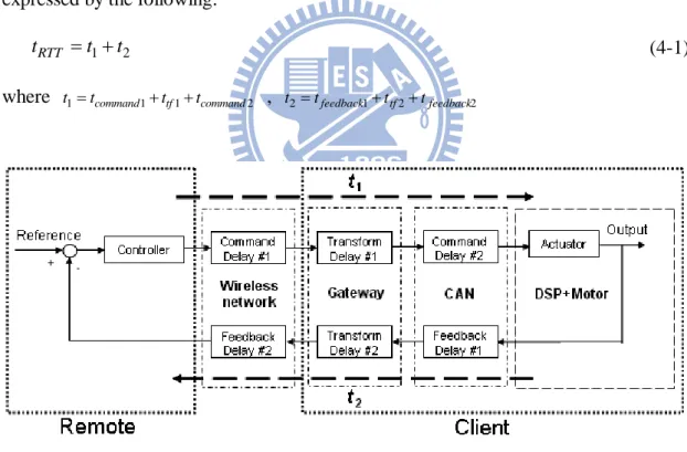
The general NCS in the closed-loop model is shown in Fig. 2.1, where t and ₁ t ₂

are the time delays induced in the network structure for the controller-to-actuator direction and the sensor-to-controller direction, respectively. Basically, the induced network delay varies according to the network load, scheduling policies, number of nodes, and different protocols. Network delay systems are also different from general linear time delay systems, where there is an assumption that the delay on the former is constant or bounded. NCS with time-varying characteristics makes modeling and design more difficult. The total time delay can be categorized into three classes based on the parts where they occur: (1) the client node, (2) the network channel, and (3) the remote node. Time delay at the client node is mainly in the preprocessing time, which is the sum of the computation, encoding, waiting, total queuing, and blocking time. Network time delay includes the total transmission time of a message and its propagation delay, which depends on the message size, data rate, and length of the network cable. Time delay at the remote node is mainly in the post-processing time, as shown in Fig. 2.1.

(26)

Fig. 2.1 The NCS block diagram

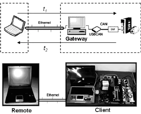
Fig. 2.2 The experimental setup

Figure 2.2 shows the structure of the present remote NCS which includes the controller in the remote node and the client for the remote-controlled device or plant. The client and the remote nodes communicate with each other from a distance through the Ethernet network. The client consists of two parts in the present experimental setup. The first part is the gateway. This is implemented in a computer with USBCAN, which is designed to communicate between the Ethernet network and the CAN bus. The second part is the local servo motor controller implemented on TI TMS320F2812 DSP with a speed-control mode. The data communication protocol adopts the TCP to construct the position loop for the remote control (Cheng et al., 2007). As shown in Fig. 2.2, the communication network can be modeled as the time

(27)

delay on the forward-command direction for actuators (t1) and on the feedback

direction for sensors (t2). Therefore, the network time delay includes both the total

transmission time of a message and the transformation time of the package from CAN to Ethernet data. The total time delay (RTT) can be expressed as tp = t1 + t2 (Fig. 2.2).

Fig. 2.3 The package transition diagram

These two protocols, Ethernet and CAN, cannot communicate with each other directly. Thus, message packages have to be processed through a gateway, as shown in Fig. 2.2. When data are transmitted to the remote node from the local hardware DSP, the type and the transmission data in a data frame should be set up in advance (Fig. 2.3). These data are then included into the CAN package and transmitted to the gateway through the CAN network, as indicated in step 1 of Fig. 2.3. After the gateway has received the package from the CAN network, the data of the CAN package will be included in the Ethernet package and the Ethernet network may thus transmit the package directly (step 2 in Fig. 2.3). When the remote node has received the package from the Ethernet network, part of the CAN package will be extracted from the Ethernet package and the data defined by users can be further obtained. In the end, the data frame will be analyzed and transmitted (step 3 of Fig. 2.3). By following the procedure (1) (2) (3), the message of the local DSP can be transmitted to a remote node. On the contrary, when data are transmitted to the remote node from the DSP, both transmission data in the data frame should be set up in the CAN package. The CAN message is then included in the Ethernet package and part of the data will be transmitted to the gateway through the Ethernet network (step 4 of Fig. 2.3). After the gateway receives the package from the Ethernet network, the data from the CAN

(28)

package will be extracted from the Ethernet package. The CAN network will be utilized to transmit this package to DSP (step 5 of Fig. 2.3). After DSP receives the package from the CAN network, the data frame in the CAN package will be extracted. This is step 6 in following the procedure (4) (5) (6) shown in Fig. 2.3.

The network time delay for the present experiments includes the following cases: (1) NCTU Laboratory NCTU Laboratory and (2) NCTU Laboratory Hukuo (the two places are 15 Km apart). The computer used for this network transmission has the following specifications: Intel® Pentium CPU 1.60 GHz, 496 MB of RAM, Realtek RTL8139/810x Family Fast Ethernet NIC Network Card, and Windows XP Professional Version 2002 OS with SP2. The local area network (LAN) is used with the time delay between the application layer of the client and remote nodes. In addition, the RTT measurement is crucial in obtaining accurate delay measurements periodically. Technically, the Windows Forms Timer component in the operating system is single threaded and is limited to an accuracy of 55 ms. A higher resolution performance counter of the DSP timer with an accuracy of 1 ms is used to measure network delay between the remote and the client nodes. We measured the time delay from two different clients within the NCTU Laboratory, and from two different clients located each in the NCTU Laboratory and Hukuo, separately, as shown in Fig. 2.4 (a) and (b). The delay time in the integrated Ethernet and the CAN Bus within a 20 ms sampling period was measured, as shown in Fig. 2.4. Only a very small time delay (around 3–15

ms) was recorded because the transmission speed of the intranet was at 100 Mbps and

there was only a relatively short route within the NCTU Laboratory. From the NCTU Laboratory to Hukuo, the delay time increases because the transmission procedure takes more routes and switches. Experimental results as shown in Fig. 2.4 indicate that the application environment greatly affects the induced delay time in NCS. Moreover, as distance increases, the delay time of a network increases as more nodes are involved.

(29)

0 2 4 6 8 10 12 14 16 18 20 0 2 4 6 8 10 12 14 16 18 20 Sec. Ti m e D e la y ( m s )

(NCTU Lab<=>NCTU Lab)

(a) 0 2 4 6 8 10 12 14 16 18 20 0 20 40 60 80 100 120 140 160 180 200 Sec. Ti m e D e la y ( m s ) (NCTU Lab<=>Hukuo) (b)

Fig. 2.4 Measured Internet delays (a) NCTU Lab - NCTU Lab and (b) NCTU Lab - Hukuo

2.3 Adaptive Smith predictor

The communication network can be modeled as the time delay on the forward-command direction for the actuator and on the feedback direction for the sensor as shown below:

(30)

Fig. 2.5 The simplified block diagram of NCS

In Fig. 2.5, t1 is the command delay time, t2 is the feedback delay time, and Gc(s) is the controller. Gp(s) denotes the transfer function of the real plant model without the delay time. The transfer function from input r to output y is obtained as follows:

s t P C s t P C s t t P C s t P C p e s G s G e s G s G e s G s G e s G s G s R s Y          ) ( ) ( 1 ) ( ) ( ) ( ) ( 1 ) ( ) ( ) ( ) ( 1 2 1 1 ) ( (2-1) where tp = t1 + t2.

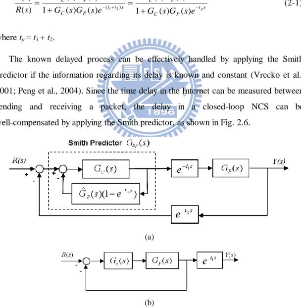
The known delayed process can be effectively handled by applying the Smith predictor if the information regarding its delay is known and constant (Vrecko et al., 2001; Peng et al., 2004). Since the time delay in the Internet can be measured between sending and receiving a packet, the delay in a closed-loop NCS can be well-compensated by applying the Smith predictor, as shown in Fig. 2.6.

(a)

(b)

Fig. 2.6 The system with the Smith predictor (a) the original system and (b) the equivalent system

(31)

Fig. 2.7 The block diagram of the adaptive Smith predictor with a PI controller

The nominal delay time and system model adopted for the Smith predictor is tm and

ˆ ( )_p

G s , respectively. In ideal conditions, Gˆ ( )_p s G_p( )s and tm= tp, the block diagram in Fig. 2.6(a) can be simplified into Fig. 2.6(b) with an additional pure time delay term applied for the Smith predictor. In this study, the delay time is estimated from the real-time measured RTT for the Smith predictor. To cope with significant variation in the delay time due to network transmission, an adaptive method is proposed for the present remote control systems with the integration of the Smith predictor, the PI controller, and the real-time delay estimation, as shown in Fig. 2.7.

2.3.1 On-line estimation of the delay time

A method for estimating the delay time within the Internet for the NCS

architecture with a combination of the time-driven and event-driven processes is proposed in this section. The designed control algorithm is realized on the present network by integrating both the Ethernet and the CAN bus with a serial data communications bus in-between. Technically, the standard CAN bus transmits only 8 bytes per frame. However, the minimum data length to realize the proposed RTT measurement is 9 bytes. A programming method wherein messages will be divided into two parts and each part will be sent at each half sampling period through the CAN network is proposed here, as shown in Fig. 2.8.

(32)

Fig. 2.8 The CAN data frame in the proposed NCS for measuring RTT

To illustrate the estimation of the induced network time delay from the measurement of RTT, the NCS transmission is shown in Fig. 2.9. At the beginning of the sampling period, the clock-driven sensor node transmits the sampling data to the controller node. By assuming the sensor-to-controller delay as t2 for this setup, the

event-driven controller node uses the sensor data to compute the control signal and then transmits it to the actuator node. By assuming the controller-to-actuator delay as

t1, the time-driven transmission is applied. The measurement of RTT is adopted due to its easy implementation and the fact that no clock synchronization is required because all computations are operated in the same device. The RTT measurement is crucial in providing accurate delay measurements periodically. A higher resolution performance counter of the DSP timer is used to measure the network delay between the remote and client nodes, as shown in Fig. 2.5. A real-time method for estimating the delay time in the Internet is proposed with all measurements for counters, indices, and delays denoted as

 Sc : sending counter

 Rc : receiving counter

 N : number of packets

 i : index of a sequence number, i 1, 2, . . . , .N

 t i_p[ ] : round-trip delay measurement of the i-th packet, using counter and i1,2, . .. ,N.

t i_p[ ]S i_c[ ]R i_c[ ]

An example of message transmission based on a 20 ms sampling time is shown in Fig. 2.9(b). If the time delay is less than one sampling time, its effect on control performance is one-sample delay. Moreover, the first frame is in normal transmission. The second frame is sent 20 ms later and a packet is received at 68 ms. The corresponding RTT is 48 ms. There is no data frame received at the sampling times of

(33)

40 and 60 ms. This phenomenon is called vacant sampling (Halevi and Ray, 1998). Two data messages (2 and 3) arrive in the same sampling period. However, only the most recent data message is used while the other data are discarded. This is referred as message rejection (Halevi and Ray, 1998; Chow and Tipsuwan, 2001). For messages 4–8, all data arrive sequentially at each sampling point, although the exact receiving time varies slightly. This occurrence is similar to delayed transmission. In summary, the delay time of NCS can be modeled using four phenomena: normal transmission, vacant sampling, message rejection, and delayed transmission. The time delay tm adopted for the adaptive Smith predictor is estimated from the measured RTT (tp) with the following rules:

(1) Normal transmission:

When the time delay is less than one sampling period, its delay effect is negligible and the measured RTT is directly adopted as tm.

(2) Vacant sampling:

When the data message is not received before occurrence of the next sampling period, the previous measured RTT added with one sampling period is recognized as the current estimation of the delay time tm.

(3) Message rejection:

When more than two data messages arrive at the same sampling period, only the most recently measured RTT is adopted as tm and all the previous measured data are discarded.

(4) Delayed transmission:

The continuously measured RTT is the estimated time delay and is directly adopted for the time delay compensation.

(34)

(b)

Fig. 2.9 The illustrative example for the time-delay estimation: (a) the architecture of the proposed RTT measurement, and (b) the four transmitted models for the RTT and the time delay estimation

2.3.2 Adaptive Smith predictor design

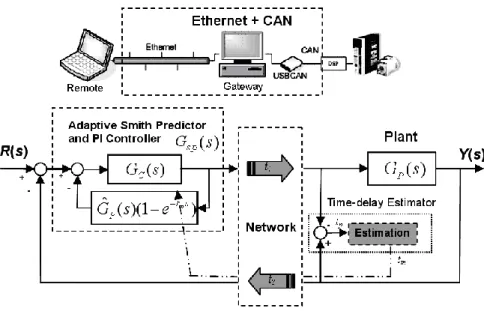
Fig. 2.10 shows the block diagram of the network control system with a time delay estimator. The total time of the command delay time and the feedback delay time is tp. The Smith predictor is proposed as a control structure to compensate for the delay time in NCS (Vrecko et al., 2001; Peng et al., 2004). As shown in Fig. 2.10, Gˆ sp( ) is

the nominal model of the system without the delay time. The transfer function for the system with the adaptive Smith predictor is expressed as follows:

1 1 2 1 ( ) ( ) ( ) ( ) ˆ ( ) 1 ( )(1 ) ( ) ( ) ( ) ( ) ( ) ˆ ˆ 1 ( ) ( ) ( ) ( ) ( ) ( ) m p m t s c P t s t t s P c c P t s c P t s t s c P c P c P G s G s e Y s R s G s e G s G s G s e G s G s e G s G s G s G s e G s G s e                (2-3)

In Fig. 10, the part of Gsp( )s with the dotted line is the Smith predictor. Its transfer function is simplified as follows:

( ) G (s) ˆ 1 (1 m ) ( ) ( ) c sp _{t s} P c G s e G s G s    (2-4)

(35)

When Gˆ_p(s)G_p(s) and t_m t_p, then the Eq. (2.3) simply becomes 1 ( ) ( ) ( ) ( ) 1 ( ) ( ) c p t s c p G s G s Y s e R s G s G s    (2-5)

Equation (2-5) shows that the transfer function when combined with the delay time and the system model transforms to two simple parts as the adaptive Smith predictor is adopted. The first part is the transfer function of the system without time delay, while the other is pure time delay. The equivalent block diagram of Eq. (2-5) is also shown in Fig. 2.6(b). Here, the system presents the same closed-loop system but only with the pure command (forward) delay time as t1. In this case, the adaptive Smith predictor is

applied because the network delay is significant and the nominal value of the delay time is adopted directly from the estimated value tm from the measured RTT.

Fig. 2.10 The control structure with the adaptive Smith predictor

2.4 Experimental results

The experimental setup was implemented to verify the effect of time delay induced by the network. To apply a remote control system on an AC 400W servo motor, both the proposed adaptive Smith predictor control method and the on-line time delay estimation algorithm were implemented efficiently on the DSP micro-controller. The position control loop is located on the remote/client site. Due to the high encoder gain of 10000 P/R, coefficients of the PI controller are tuned as

0001 . 0  p K andK_i 0.00000001.

(36)

0 0.1 0.2 0.3 0.4 0.5 0.6 0.7 0.8 0.9 1 -200 0 200 400 600 800 1000 1200 Time (sec.) S pe ed ( rp m /m in ))

Command Actual output response Estimated Model respone

Fig. 2.11 Experimental results for system identification

The system identification result of the speed-control loop from the pseudo-random binary signal (PRBS) response for the present AC permanent magnet synchronous motor is shown in Fig. 2.11. The open positional loop is identified as

) 1 019 . 0 0001 . 0 ( ) 221 . 3 058 . 0 ( 10 ) ( ₂ 4     s s s s s GP

Different controllers were tested as follows: (1) the PI controller only, (2) the Smith predictor with the PI controller designed with a fixed delay time, and (3) the adaptive Smith predictor with the PI controller. For the client, the sampling time of the experiments was 20 ms with a square-wave command. The upper/lower commands of 30,000/15,000 pulses were provided. As the delay time increases (Fig. 2.12(d)), simulation results indicate that the control performance of the proposed adaptive Smith predictor presents the best performance compared with the PI controller and the Smith predictor. Experiments were also set up with different sites to test the proposed design. The delay time within the NCTU Laboratory is much smaller than the sampling time. Hence, the effect of time delay is negligible as shown in Fig. 2.13(d). Experimental results indicate that the control performance for different controllers is similar if the delay is small (Fig. 2.13).

(37)

0 5 10 15 0 1 2 3 4 5x 10 4 _{PI Controller} Sec. P o s it io n ( p u ls e ) (a) 0 5 10 15 0 1 2 3 4 5x 10

4 _{Classical Smith Predictor with PI Controller}

Sec. P o s it io n ( p u ls e ) (b) 0 5 10 15 0 1 2 3 4 5x 10

4 _{Adaptive Smith Predictor with PI Controller}

P o s it io n ( p u ls e ) Sec. (c) 0 5 10 15 0 200 400 600 Sec. Ti m e d e la y ( m s ) (d)

Fig. 2.12 Simulation results for (a) the PI controller, (b) the Smith predictor (tm=200 ms) with

(38)

0 2 4 6 8 10 12 14 16 18 20 0 0.5 1 1.5 2 2.5 3 3.5 4x 10 4 Sec. Po si tio n (p ul se )

PI Controller (NCTU Lab<=>NCTU Lab)

(a) 0 2 4 6 8 10 12 14 16 18 20 0 0.5 1 1.5 2 2.5 3 3.5 4x 10 4 Sec. P os iti on (p ul se )

Classical Smith Predictor with PI Controller (NCTU Lab<=>NCTU Lab)

(b) 0 2 4 6 8 10 12 14 16 18 20 0 0.5 1 1.5 2 2.5 3 3.5 4x 10 4 Sec. P os iti on (p ul se )

Adaptive Smith Predictor with PI Controller (NCTU Lab<=>NCTU Lab)

(c) 0 2 4 6 8 10 12 14 16 18 20 0 5 10 15 20 Sec. Ti m e De lay (m s)

(NCTU Lab<=>NCTU Lab)

(d)

Fig. 2.13 Experimental results on Intranet (NCTU LabNCTU Lab) (a) PI controller, (b) Smith predictor (tm=5 ms), and (c) adaptive Smith predictor

(39)

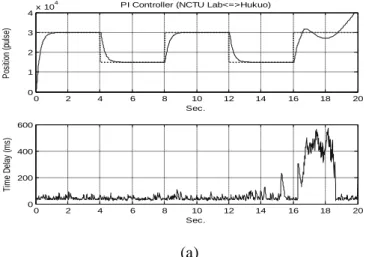
0 2 4 6 8 10 12 14 16 18 20 0 1 2 3 4x 10 4 Sec. P os iti on ( pu ls e)

PI Controller (NCTU Lab<=>Hukuo)

0 2 4 6 8 10 12 14 16 18 20 0 200 400 600 Sec. Ti m e D el ay ( m s) (a) 0 2 4 6 8 10 12 14 16 18 20 0 1 2 3 4x 10 4 Sec. P os iti on ( pu ls e)

Classical Smith Predictor with PI Controller (NCTU Lab<=>Hukuo)

0 2 4 6 8 10 12 14 16 18 20 0 200 400 600 Sec. Ti m e D el ay ( m s) (b) 0 2 4 6 8 10 12 14 16 18 20 0 1 2 3 4x 10 4 Sec. P o s it io n ( p u ls e )

Adaptive Smith Predictor with PI Controller (NCTU Lab<=>Hukuo)

0 2 4 6 8 10 12 14 16 18 20 0 200 400 600 Sec. Ti m e D e la y ( m s ) (c)

Fig. 2.14 Experimental results on Internet (NCTU LabHukuo, 15 Km) (a) PI controller, (b) Smith predictor (t_m= 46 ms), and (c) adaptive Smith predictor

(40)

0 0.2 0.4 0.6 0.8 1 1.2 1.4 1.6 1.8 2 0 1 2 3 4 5x 10 4 Sec. P o s it io n ( p u ls e )

Fig. 2.15 Experimental results for the adaptive Smith predictor (without the initial delay)

0 0.2 0.4 0.6 0.8 1 1.2 1.4 1.6 1.8 2 0 1 2 3 4 5x 10 4 Sec. P o s it io n ( p u ls e )

Fig. 2.16 Experimental results for the adaptive Smith predictor (with the initial time delay)

For the experiments tested between the NCTU Laboratory and Hukou, which had 15 Km distance and massive download data at 16 seconds from multiple users sharing the limited network bandwidth, the results indicate that the time delay increases accordingly to a certain level. Moreover, the PI controller with a fixed-delay Smith predictor becomes unsuitable, as shown in Figs. 2.14(a) and (b). However, even with the dramatically varied network-induced time delay, the proposed adaptive Smith predictor still renders improved performance as shown in Fig. 2.14(c). Compared with the three continuous responses of the proposed adaptive Smith predictor without considering the initial value as shown in Fig. 2.15, the proposed design with proper initial delay time renders much improved performance as shown in Fig. 2.16.

2.5 Summary

In this chapter, the remote control system was realized on the integrated Ethernet and CAN bus. By applying the adaptive Smith predictor with an on-line estimator for

(41)

the time delay, the significantly induced time delay effect on the NCS was successfully reduced. Experimental results are summarized as follows:

(1) Since the present network integrates both the Ethernet and the CAN bus, the transmitted message is restricted by the CAN frame because its data length is limited to 8 bytes per frame only. For real-time applications, the present measurement of RTT requires 9 bytes for the data length. Therefore, in this study, an algorithm is proposed by sending the measurement of each frame at the half sampling period to achieve on-line estimation of the delay time for the proposed NCS.

(2) The adaptive Smith predictor is adopted with the on-line estimated time delay to achieve improved performance of NCS. The significant time-varying delay effect mainly on the Ethernet is thus reduced. Experimental results on an AC servo motor over 15 Km away also indicate that the proposed approach leads to significantly improved stability and control performance. (3) The present remote controller applying the adaptive Smith predictor may

present a larger overshoot because the initial estimation error exists. By measuring the time delay in advance as the initial value in the adaptive Smith predictor, better performance can thus be obtained.

Although the remote control system with a general NCS is stable for most of the time because the varied delay is bounded, system stability is not guaranteed especially when a serious time delay occurs. To prove the feasibility of the proposed approach, the adaptive Smith predictor was successfully applied to NCS under significantly time-varying delay time to control an AC servo motor.

(42)

Chapter 3 Robust NCS Design

Most NCS control designs are based on the nominal system model. However, modeling error and disturbance exist in real environments. The robust NCS design is proposed to cope with both the time varied delay and the external loading in this chapter. Compared with commercial networks, industrial networks in the NCS usually present minor variation in the time delay; on the other hand, the commercial Internet usually presents significant time delay. A template expressed as the phase and gain for the quantitative feedback theory (QFT) design has been constructed by considering the bounded variations with the time delay and the external loading. In addition, as the significant time delay of the NCS occurs over the wired Ethernet, the adaptive Smith predictor with QFT controller can be suitably adopted by employing the proposed online estimated RTT. Both simulation and experimental results on AC servo motor with the integrated CAN bus and the Ethernet have proven feasibility and improved performance of the proposed robust NCS.

3.1 The varied time delay effect

Most robust methods assume that the varying delay is relatively smaller than the system sampling time without considering the critical vacant sampling or message rejection (Halevi and Ray, 1998); however, these phenomena happen frequently in real applications. The reported robust design approaches face difficulties in NCS realization especially in the remote control system combining the industrial CAN bus and the commercial Ethernet. As shown in Fig. 2.2, the present NCS is mainly comprised of the remote node and the client node. They communicate with each other from a distance through the Ethernet network. The client at a location includes two parts. The first part is the gateway to computer communication with the USBCAN, which is designed to communicate between the Ethernet network and the CAN bus (Cheng et al., 2007). The gateway is linked with TI TMS320F2812 DSP through the CAN network, and the remote site is linked via the Ethernet network. The second part is the servo motor controller implemented on TI TMS320F2812 DSP with a speed-control

(43)

mode. Finally, the data communication protocol adopts the TCP to achieve the desirable position loop control for the guaranteed eventual delivery of packets. This research considers the delay time to be the RTT, which is the required period for a packet to travel from the client node to the remote node and back to the original client node. The delay measurement relies on the RTT due to its easy implementation, and no clock synchronization is required as all computations are running in the same device (Vatanski et al., 2009). In Fig. 3.1, the comparison of the results between the CAN bus and Ethernet network obviously shows that the time delay in the Ethernet network remains the bottleneck during the transmission for the NCS.

0 1 2 3 4 5 6 7 8 9 10 0 50 100 150 R TT ( m s ) Second Remote <-> DSP, Ethernet+CAN Gatew ay <-> DSP, CAN

Fig. 3.1 Measured time delay

The time delay occurs between the application layer of the plant and the application layer of the gateway, and it is measured mainly from the plant to the client, which implements different network services (ADSL, Cable modem, and Intranet). Packets with different lengths whose payloads consist of a sequence number were sent out at periodic intervals. Experimental results as shown in Fig. 3.1 indicate that the time delay in the CAN bus is relatively small and stable compared with that of the Ethernet network, which is greatly affected by its environments, as shown in Table 3.1. Moreover, as the transmission rate decreases and the sampling period increases, the

(44)

delay time of the network increases dramatically. Furthermore, as shown in Fig. 3.2, the measured drifting time delay presents both bounded and random natures.

Table 3.1 The averaged delay time for the Ethernet and CAN networks (1000 Samples, Unit: ms)

Network delay time

(ms)

Sampling Time (ms) Intranet (10 Mbps) Cable Modem (6 Mbps) ADSL (2 Mbps) 5 35.741 198.843 380.424 10 31.819 153.257 372.496 15 27.235 135.932 298.991 20 25.740 130.926 276.215 0 1 2 3 4 5 6 7 8 9 10 11 12 13 14 15 16 17 18 19 20 20 40 60 80 100 120 140 160 180 200 Ti m e D e la y ( m s ) Second (a) 0 1 2 3 4 5 6 7 8 9 10 11 12 13 14 15 0 100 200 300 400 500 600 700 800 900 Ti m e D e la y ( m s ) Second (b)

Fig. 3.2 The time delay effect measured RTT at (a) 9:00 am, and (b) 12:00 pm

3.2 QFT design

The previous experiments indicate that network time delay has two characteristics: (1) bounded and (2) drifting. For the bounded delay, a robust QFT design with a suitable plant template is proposed in this study. The frequency-response template for a class of transfer functions with the time-varying delay in the phase and with the payload variation in the gain is likewise proposed. For the drifting delay, an adaptive Smith predictor control scheme integrated with the QFT controller is proposed. The

網路控制系統之時間延遲補償設計

國

立

交

通

大

學

電控工程研究所

博

士

論

文

網路控制系統之時間延遲補償設計

Networked Control Systems Design with the

Time Delay Compensation

研 究 生：賴 建 良

網路控制系統之時間延遲補償設計

研究生

:

賴建良 指導教授

:

徐保羅 博士

國立交通大學

電控工程研究所

摘 要

Networked Control Systems Design with the

Time Delay Compensation

Student : Chien-Liang Lai Advisor : Dr. Pau-Lo Hsu

Institute of Electrical and Control Engineering

National Chiao Tung University

ABSTRACT

Acknowledgment

Table of Contents

List of Figures

List of Tables

Chapter 1

Introduction

1.1 General review

1.2 Model-based NCS control design

1.3 Problem statement

1.4 Proposed approach

1.5 Contributions

1.6 Contents overview

Chapter 2

On-line Time-delay Estimation Design

2.1

Introduction

2.2

NCS and time-delay measurement

2.3

Adaptive Smith predictor

2.4

Experimental results

2.5

Summary

Chapter 3

Robust NCS Design

3.1

The varied time delay effect

Network delay time

3.2

QFT design

研究生：賴建良

賴建良指導教授

徐保羅博士

摘要