用於時變通道下有限回饋傳送波束形成之基於吞吐量模式選擇準則

國立交通大學

電信工程學系碩士班

碩士論文

用於時變通道下有限回饋傳送波束形成之

基於吞吐量模式選擇準則

Throughput-Based Mode Selection Criterion for

Limited-Feedback Transmit Beamforming over

Time-Varying Channels

用於時變通道下有限回饋傳送波束形成之基於吞吐量

模式選擇準則

Throughput-Based Mode Selection Criterion for

Limited-Feedback Transmit Beamforming over

Time-Varying Channels

研 究 生 : 張亦杰 Student:

Yi-Chieh

Chang

指導教授 : 李大嵩 博士 Advisors: Dr. Ta-Sung Lee

吳卓諭 博士

Dr. Jwo-Yuh Wu

國立交通大學

電信工程學系碩士班

碩士論文

A Thesis

Submitted to Department of Communication Engineering

College of Electrical and Computer Engineering

National Chiao Tung University

in Partial Fulfillment of the Requirements

for the Degree of

Master of Science

in

Communication Engineering

June 2009

Hsinchu, Taiwan, Republic of China

用於時變通道下有限回饋傳送波束形成之基於

吞吐量模式選擇準則

研 究 生 : 張亦杰

指導教授：李大嵩 博士

吳卓諭 博士

國立交通大學電信工程學系碩士班

摘要

在 本 篇 論 文 中 ， 吾 人 考 慮 適 用 於 時 變 通 道 環 境 之 多 輸 入 單 輸 出 （ Multiple-Input Single-Output, MISO ） 有 限 回 饋 預 編 碼 (Limited Feedback Precoding) 系統的雙模式編碼方法，吾人持用之通道模式係由一階馬可夫通道模 型描述。因為通道統計特性隨著時間碼框改變，系統需提供不同大小的碼書以提 升性能表現。在吾人的系統中，採用的兩種不同的碼書係遵循 IEEE 802.16e 標 準之定義，並分別對應到不同的通道向量量化程度。基於公平原則，系統中的雙 模式具有相同的平均回傳率。為了在不同的通道相關性下選擇適當的碼書，吾人 提出一個以吞吐量為準則的模式選擇方法協助接收機決定使用的碼書類型。吾人 亦提出實際可行的準則實現模式及選擇方法供接收機使用。模擬顯示吾人所提出

Throughput-Based Mode Selection Criterion for

Limited-Feedback Transmit Beamforming over

Time-Varying Channels

Student: Yi-Chieh Chang

Advisor: Dr. Ta-Sung Lee

Dr.

Jwo-Yuh

Wu

Department of Communication Engineering

National Chiao Tung University

Abstract

In this thesis, we consider a dual-mode precoding method for limited-feedback multiple-input single-output (MISO) systems over time-varying channels, which follows the first-order Markov channel model. Since the channel statistics varies over time frames, codebooks of different sizes should be available to improve the system performance. In the considered system, there are two codebooks corresponding to different quantizations of channel vectors as adopted in the IEEE 802.16e standard. For fairness, the two modes have the same feedback rates. To choose one suitable mode for use under different channel correlations, we propose a throughput-based mode selection criterion to help the receiver decide the codebook to be used. A practical way to implement the criterion at the receiver is also proposed. Simulations indicate that the proposed scheme is superior to that with a single codebook and perform comparably to those existing mode selection criteria.

Acknowledgement

I would like to express my deepest gratitude to my advisors, Dr. Ta-Sung Lee and Dr. Jwo-Yuh Wu, for their training of oral presentation and prudent attitude toward research. Moreover, I learned a lot from their positive attitude in many areas. Thanks are also offered to all members in the Communication System Design and Signal Processing (CSDSP) Lab.

At last but not least, I would like to show my sincere thanks to my family for their invaluable love and support.

Contents

Contents...IV

List of Figures ...VI

List of Tables ...VIII

Acronym Glossary ...IX

Notations... X

Chapter 1 Introduction ... 1

Chapter 2 System Model ... 4

2.1 Limited Feedback in MISO System...5

2.2 Time-Varying Channel Model ...6

2.3 Codebook Construction ...8

2.4 Summary ...14

Chapter 3 Dual-Mode Scheme and Mode Selection ... 15

3.1 Dual-Mode Scheme ...16

3.2 Throughput-Based Criterion ...17

3.3 Modal Metric ...18

3.3.1 Computation of Modal Metric in Mode I ...19

3.3.2 Computation of Modal Metric in Mode II ...21

3.4 Selection of Good Mode and Beamformer ...25

3.6 Summary ...28

Chapter 4 Modal Metric Approximation... 29

4.1 Approximation of Modal Metric in Mode I...30

4.2 Approximation of Modal Metric in Mode II...34

4.3 Numerical Results...37

4.3.1 Approximation vs. Exact Value (Mode I) ...38

4.3.2 Approximation vs. Exact Value (Mode II)...39

4.3.3 Dual-Mode Scheme vs. Single-Mode Scheme ...41

4.3.4 Throughput-Based Criterion vs. Other Criteria ...43

4.4 Summary ...45

Chapter 5 Conclusion ... 46

List of Figures

Fig. 2-1 MISO system model...6

Fig. 2-2 Power spectrum of first order AR process with a = 0.22 ...7

Fig. 3-1 Dual-mode selection scheme in MISO system ...16

Fig. 3-2 Histogram of the random variable V and its approximation with Gamma distribution ...23

Fig. 3-3 The RMSE of using ( )f v and using different order of polynomials ...23

Fig. 3-4 Joint PDF of random variables V and U ...24

Fig. 3-5 Product of PDFs of random variables V and U ...24

Fig. 3-6 Flow chart of selecting a mode and a beamformer ...25

Fig. 3-7 Dual-mode scheme and single-mode scheme with SNR = 10dB and 16 QAM ...27

Fig. 4-1 T vs. ₁ T with 16 QAM and different channel correlations ...38 ₁* Fig. 4-2 T vs. ₁ T with 64 QAM and different channel correlations ...39 ₁* Fig. 4-3 T vs. ₂ T with 16 QAM and different channel correlations ...40 ₂* Fig. 4-4 T vs. ₂ T with 64 QAM and different channel correlations ...40 ₂* Fig. 4-5 Dual-mode scheme, Dual-mode scheme with approximated modal metric and single-mode scheme with SNR = 10dB and 16 QAM...42

Fig. 4-6 Dual-mode scheme, Dual-mode scheme with approximated modal metric and single-mode scheme with SNR = 10dB and 64 QAM...42

Fig. 4-8 Throughput-based criterion and SER-based criterion in the dual-mode scheme with SNR = 10dB and 16 QAM...44 Fig. 4-9 Throughput-based criterion and SER-based criterion in the dual-mode scheme with SNR = 10dB and 16 QAM...44

List of Tables

Table 2-1 Transmit beamforming codebooks in IEEE 802.16-2005 standard...8

Table 2-2 MIMO precoding codebook V(2,1, 3)...8

Table 2-3 MIMO precoding codebook V(3,1, 3)...9

Table 2-4 MIMO precoding codebook V(4,1, 3)...9

Table 2-5 Generating parameters for V(3,1, 6) and V(4,1, 6)...10

Table 2-6 MIMO precoding codebook V(3,1, 6)... 11

Table 3-1 Simulation parameters ...26

Acronym Glossary

BER bit error rate

CSI channel state information

IEEE institute of electrical and electronics engineers MIMO multiple-input multiple-output

MISO multiple-input single-output PDF probability density function QAM quadrature amplitude modulation SER symbol error rate

Notations

Es average symbol energy [ ]⋅

E expectation operator

k

f unit precoder for the k th frame

s

f selected precoder for maximizing the throughput

1 F 3-bit codebook 2 F 6-bit codebook H k

h MISO channel vector for the k th frame

0( )

I i modified Bessel function of the first kind of zero order

, ( )

a b

M ⋅ _{Wittaker function}

k

n _{complex Gaussian noise for the k th frame} t

N number of transmit antennas ( )

M

P γ symbol error rate for M -QAM modulation

k

s _{transmitted symbol at the k th frame} ( )

T γ throughput

, ( )

i j

T γ throughput for the i th frame under the j th mode

k

y _{received signal at the the k th frame} γ _{instantaneous signal-to-noise ratio}

( )

Γ ⋅ gamma function

m

Γ modal metric for the m th mode

Δh innation vector for the first-order Markov channel model ρ _{channel correlation}

( )

Chapter 1

Introduction

In wireless transmission scenarios, multiple antennas at both the transmitter and the receiver are employed to provide higher data transmission rate and lower data error rate, and this is known as multiple-input multiple-output (MIMO) systems. There are two types of scenario in MIMO systems, which are open-loop systems and closed-loop systems. For the former one, the receiver does not use channel state information (CSI), while the latter is able to acquire CSI from the receiver. Among open-loop architectures, one of the most popular approaches is the Vertical Bell Laboratories Layered Space-Time (V-BLAST) [1], which involves a simple coding technique to send data via different date streams, and hence enhance the data transmission rate. Closed-loop systems, while having CSI at the transmitter and hence increasing the complexity of the receiver, yield higher capacities and lower data error rate since the transmitted data can be pre-designed to match the channel. Limited

In multiple antenna systems, beamforming is a simple technique to improve system performance in fading channels [4, 5]. Unfortunately, this scheme needs perfect CSI, which is often not available at the transmitter side, to achieve the theoretical performance. Previous works [6-8] have investigated many ways to feed back the CSI to transmitter. For example, the mean-feedback technique is discussed in [6, 7]; the covariance-feedback approach is presented in [6, 8]. Among these works, they assume the transmitter has the knowledge of channel distribution, so the first-order and second-order statistics are fed back to improve the system performance. In this thesis, we focus on one prevailing technique in which the quantized channel vectors lying in pre-designed codebooks are fed back to the transmitter [4, 9], and this kind of scheme were adopted in systems like the IEEE 802.16e standard [10].

We consider a precoding scheme called dual-mode precoding method in [11] with a different mode selection criterion, based on throughput consideration. Under the architecture of dual-mode precoding, two codebooks containing different number of quantized channel vectors are provided at both the transmitter and the receiver. The receiver chooses not only the best precoder in terms of throughput, which will be defined in Chapter 3, but also a suitable mode for the transmitter to adopt. Here, different modes correspond to different codebooks, which in our case are 3-bit quantization codebook and 6-bit quantization codebook as adopted in the IEEE 802.16e standard [10]. As for mode selection, the modal metric exploiting channel correlation will be defined in this thesis, which is similar to that in [11]. Simulations indicate that the proposed criterion works well for the dual-mode scheme and is superior to the system having only one codebook, which we call the single-mode scheme throughout this thesis. Also, the dual-mode scheme with the proposed criterion has comparable performance to other existing criteria and is of more practical interests.

This thesis will proceed as follows. Chapter 2 describes the system model and the channel model used in our work. Also, the codebook construction in IEEE 802.16e-2005 is presented. In Chapter 3, we will give the definition of the throughput and the modal metric. Moreover, the throughput-based mode selection criterion will be defined and the computation of the modal metric with respect to Mode I and Mode II are also presented. In Chapter 4, the accurate approximations of the modal metric pertaining to the two modes will be derived, which is proved to be accurate in terms of numerical experiment. Simulations and conclusions are presented in Chapter 4 and Chapter 5, respectively.

Chapter 2

System Model

Limited feedback system was first proposed in [2, 3] and has drawn attention for many years and emerged as one of the most significant techniques in wireless communications. A great many research works have investigated its utility and justified the great performance enhancement via limited bits fed back to the transmitter. Moreover, limited feedback scheme has been employed in multiple-input multiple-output (MIMO) systems to provide higher capacity and higher reliability in recent years since channel state information (CSI) can be relayed back to the transmitter in an efficient way.

One of the greatest challenges of designing limited-feedback scheme lies in the design of codebooks. How to design codebooks so that the matrices in them can best describe the channel quality in various circumstances has been discussed and solved. In [12], the codebook design criterion in independent and identically distributed Rayleigh fading matrix channels is related to the problem of Grassmannian line packing. Also, the random vector quantization (RVQ) technique is introduced in [13] to provide a simple approach to codebook design. Moreover, a systematic codebook design for correlated channels is presented in [14].

In Chapter 2, a limited feedback scheme in MISO system is introduced first. Then, a time-varying channel model, which in our case is the first-order Markov channel model, will be given and discussed. Finally, IEEE 802.16-2005 [10] codebook construction is presented

2.1 Limited Feedback in MISO System

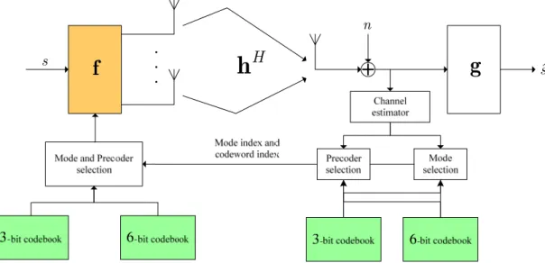
We consider a multi-input single-output (MISO) system with N transmit antennas _t and a single receive antenna, which is shown in

Fig. 2-1. The received signal can be described as

H

k k k k k

y =h f s +n (2.1)

where s is the transmitted symbol at k th frame and _k f is an _k N × unit precoder _t 1 which is selected for the same frame. Channel vector is described as

1 2

[ , , , _t]

H H H H k = h h hN

h … and h_kH ∼ CN

(

0_Nt,I_Nt

)

is distributed according to complex Gaussian distribution with zero mean and unit variance. Also, we assume the received signal experiences the noise n_k ∼ CN(0,N₀)at the receiver.

Assuming that the receiver has full knowledge of channel statistics, the instantaneous signal-to-noise ratio (SNR) in (2.1) is

2 0 H k k Es N γ = h f (2.2)

with Es denoting the average symbol energy. In the following, we will assume that 1

f

n ˆ s H

h

s

_g

Fig. 2-1 MISO system model

2.2 Time-Varying Channel Model

The channel model used in this thesis follows the first-order Markov channel model [15-17] 1 k+ = ρ k + Δ h h h (2.3) where ( ,(1 ) ) t t N ρ N

Δh ∼CN 0 − I is the innovation vector and ρ is the channel

correlation between k th and (k +1)th frame, in which k denotes a specific frame index.

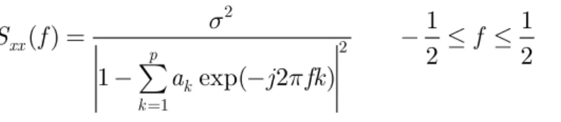
In fact, (2.3) can be viewed as a first-order autoregressive (AR) process [15], which is often used to approximate a given random process. A complex AR process can be generated via the following recursion formula

1 [ ] p _k [ ] [ ] k x n a x n k w n = =

_∑

− + (2.4)

where p is the order of AR and [ ]w n is the innovation vector, which is complex white Gaussian with zero mean and variance σ . Comparing (2.3) with (2.4), we 2 immediately verify that our channel model is equivalent to a first-order AR process.

following rational form [17]: 2 2 1 1 1 ( ) 2 2 1 exp( 2 ) xx _p k k S f f a j fk σ π = = − ≤ ≤ −

_∑

− (2.5)

which is bell-shaped (see Fig. 2-2) and can be used to approximate indoor channel models [18] -0.5 -0.4 -0.3 -0.2 -0.1 0 0.1 0.2 0.3 0.4 0.5 0.8 1 1.2 1.4 1.6 1.8 2

Hz

magnitude

Sxx(f)

2.3 Codebook Construction

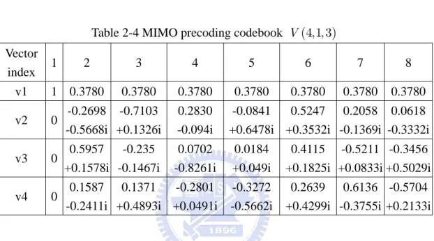
There are two kinds of codebooks defined in the the IEEE 802.16-2005 standard [10]: 3-bit codebooks and 6-bit codebooks. When both the number of input data streams and the number of the receive antennas are equal to 1, the scenario is called transmit beamforming. The transmit beamforming codebooks are listed in Table 2-1. The notation V N S L

(

_t, ,

)

denotes the vector codebook, which consists of 2L complex unit vectors of dimension N . The S denotes the number of substreams. _t All the codewords of V(2,1, 3), V(3,1, 3), and V(4,1, 3) are listed in Table 2-2, Table 2-3, and Table 2-4.

Table 2-1 Transmit beamforming codebooks in the IEEE 802.16-2005 standard , \ t N S L 3 6 2,1 V(2,1, 3) V(2,1, 6) 3,1 V(3,1, 3) V(3,1, 6) 4,1 V(4,1, 3) V(4,1, 6)

Table 2-2 MIMO precoding codebook V(2,1, 3) Vector index 1 2 3 4 5 6 7 8 v1 1 0.7490 0.7490 0.7491 0.7491 0.3289 0.0.5112 0.3289 v2 0 -0.5801 +j0.1818 0.0576 +j0.6051 -0.2978 -j0.5298 -0.6038 +j0.0689 -0.6614 +j0.6740 -0.4754 -j0.7160 -0.8779 -j0.3481

Table 2-3 MIMO precoding codebook V(3,1, 3) Vector index 1 2 3 4 5 6 7 8 v1 1 0.5 0.5 0.5 0.5 0.4954 0.5 0.5 v2 0 -0.7201 -0.3126i -0.0659 +0.1371i -0.0063 +0.6527i 0.7171 +0.3202i 0.4819 -0.4517i 0.0686 -0.1386i -0.0054 -0.654i v3 0 0.2483 -0.2684i -0.6283 -0.5763i 0.4621 -0.3321i -0.2533 +0.2626i 0.2963 -0.4801i 0.6200 +0.5845i -0.4566 +0.3374i

Table 2-4 MIMO precoding codebook V(4,1, 3) Vector index 1 2 3 4 5 6 7 8 v1 1 0.3780 0.3780 0.3780 0.3780 0.3780 0.3780 0.3780 v2 0 -0.2698 -0.5668i -0.7103 +0.1326i 0.2830 -0.094i -0.0841 +0.6478i 0.5247 +0.3532i 0.2058 -0.1369i 0.0618 -0.3332i v3 0 0.5957 +0.1578i -0.235 -0.1467i 0.0702 -0.8261i 0.0184 +0.049i 0.4115 +0.1825i -0.5211 +0.0833i -0.3456 +0.5029i v4 0 0.1587 -0.2411i 0.1371 +0.4893i -0.2801 +0.0491i -0.3272 -0.5662i 0.2639 +0.4299i 0.6136 -0.3755i -0.5704 +0.2133i

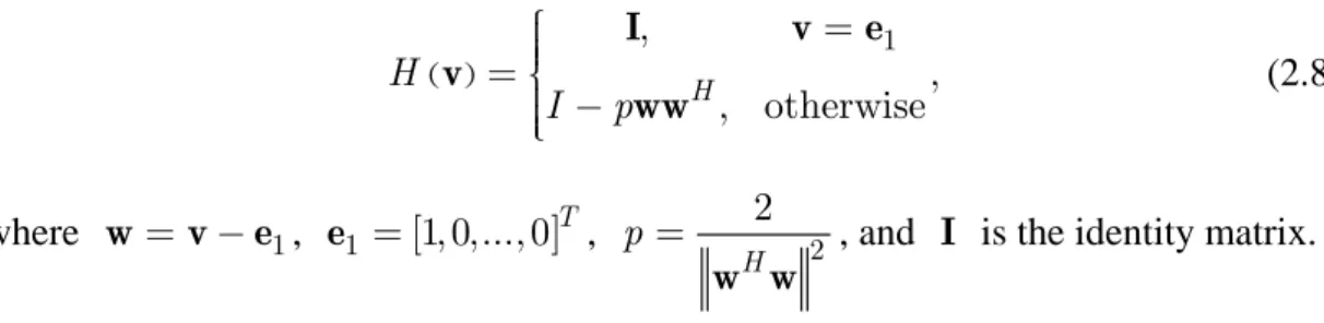
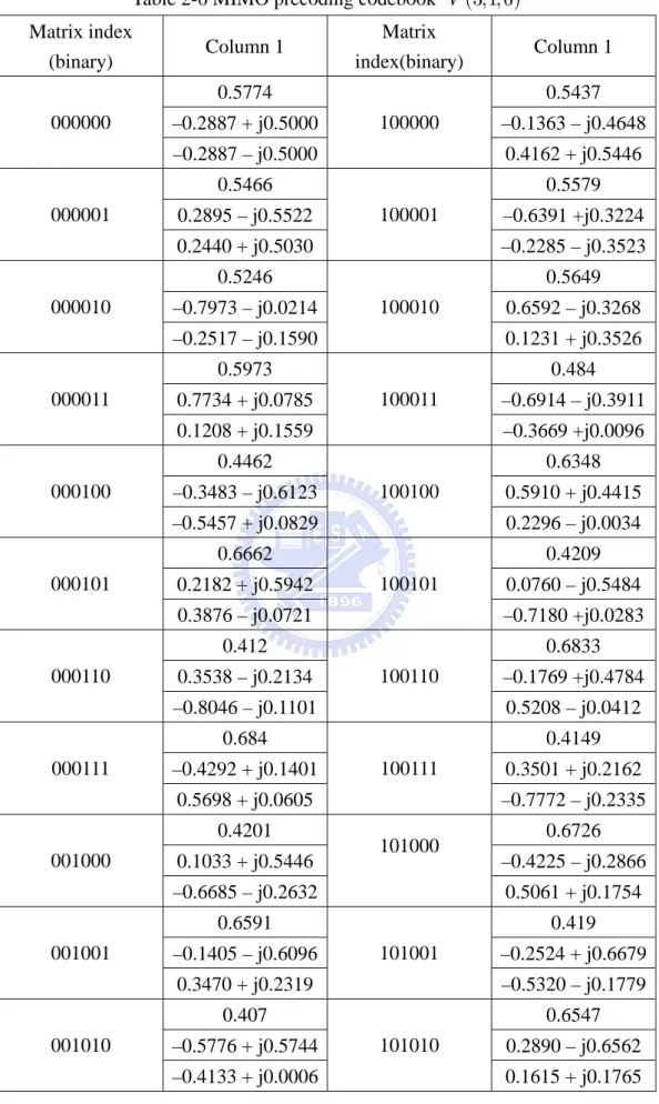
In the IEEE 802.16-2005 standard [10], two vector codebooks V(3,1, 6) and (4,1, 6)

V are generated as follows. All the vector codewords v , _i i =2,...,2L are derived from the first codeword v as ₁

1 ( ) ( )i H( ) , for 2,..,2 ,L i =H Q H i− i = v s u s v (2.6) 1_{, for 2,..,2 ,} j L i = ie−φ i = v v (2.7)

( ) 1 , , , otherwise H H I p ⎧ = ⎪⎪⎪ = ⎨ ⎪ − ⎪⎪⎩ I v e v ww (2.8) where w= −v e , ₁ e₁ =[1, 0,..., 0]T, 2 ₂ H p =

w w , and I is the identity matrix.

The parameters for the generation of V(3,1, 6) and V(4,1, 6) are listed in Table 2-5 and the codewords of V(3,1, 6) is listed in Table 2-6.

Table 2-5 Generating parameters for V(3,1, 6) and V(4,1, 6)

t N L u in ( ) i Q u s in H( )s 3 6 [1,26, 57 [] 1.2518−j0.6409, 0.4570− −j0.4974, 0.1177+j0.2360]T 4 6 [1, 45,22, 49 ] [ ] 1.3954 0.0738, 0.0206 0.4326, 0.1658 0.5445, 0.5487 0.1599T j j j j − + − − −

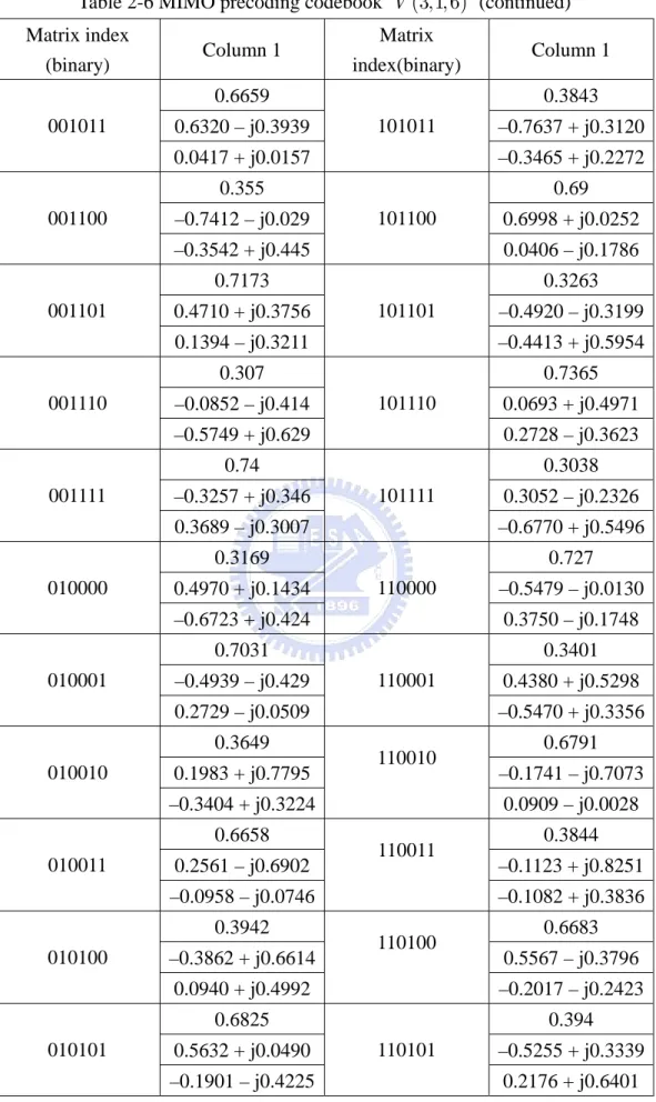
The algorithms given above can help us generate the vector codebooks (3,1, 6)

V and V(4,1, 6). But, the IEEE 802.16e-2005 standard does not provide the generating parameters for the codebook V(2,1, 6).

There are sixty-four precoders in the 6-bit codebook to be selected. Therefore it has a higher probability that a near-optimal precoder can be selected. But the receiver needs to feed back six bits per CSI update. On the other hand, although the 3-bit codebook provides only eight beamformers to be selected, the feedback amount per CSI update is only three bits.

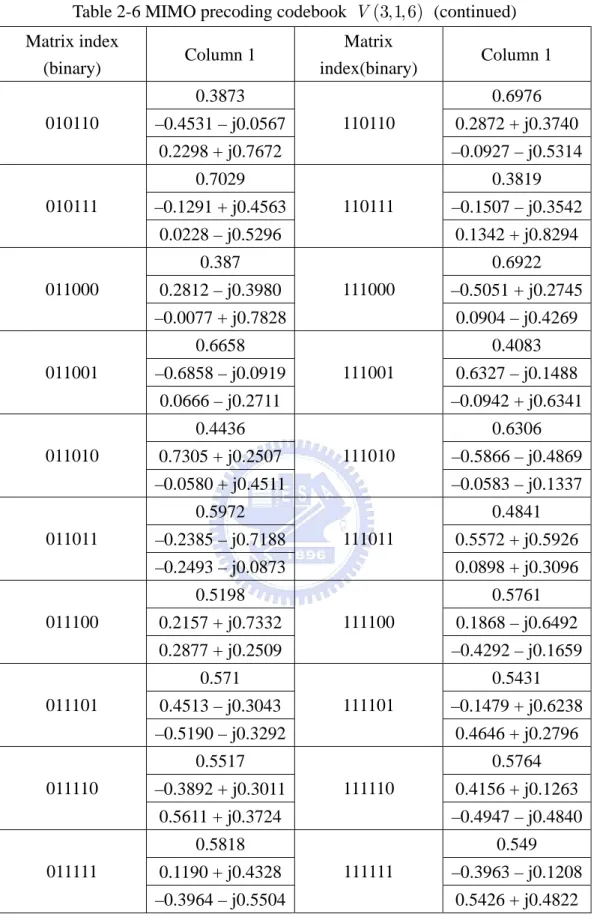
Table 2-6 MIMO precoding codebook V(3,1, 6) Matrix index (binary) Column 1 Matrix index(binary) Column 1 0.5774 0.5437 –0.2887 + j0.5000 –0.1363 – j0.4648 000000 –0.2887 – j0.5000 100000 0.4162 + j0.5446 0.5466 0.5579 0.2895 – j0.5522 –0.6391 +j0.3224 000001 0.2440 + j0.5030 100001 –0.2285 – j0.3523 0.5246 0.5649 –0.7973 – j0.0214 0.6592 – j0.3268 000010 –0.2517 – j0.1590 100010 0.1231 + j0.3526 0.5973 0.484 0.7734 + j0.0785 –0.6914 – j0.3911 000011 0.1208 + j0.1559 100011 –0.3669 +j0.0096 0.4462 0.6348 –0.3483 – j0.6123 0.5910 + j0.4415 000100 –0.5457 + j0.0829 100100 0.2296 – j0.0034 0.6662 0.4209 0.2182 + j0.5942 0.0760 – j0.5484 000101 0.3876 – j0.0721 100101 –0.7180 +j0.0283 0.412 0.6833 0.3538 – j0.2134 –0.1769 +j0.4784 000110 –0.8046 – j0.1101 100110 0.5208 – j0.0412 0.684 0.4149 –0.4292 + j0.1401 0.3501 + j0.2162 000111 0.5698 + j0.0605 100111 –0.7772 – j0.2335 0.4201 0.6726 0.1033 + j0.5446 –0.4225 – j0.2866 001000 101000

Table 2-6 MIMO precoding codebook V(3,1, 6) (continued) Matrix index (binary) Column 1 Matrix index(binary) Column 1 0.6659 0.3843 0.6320 – j0.3939 –0.7637 + j0.3120 001011 0.0417 + j0.0157 101011 –0.3465 + j0.2272 0.355 0.69 –0.7412 – j0.029 0.6998 + j0.0252 001100 –0.3542 + j0.445 101100 0.0406 – j0.1786 0.7173 0.3263 0.4710 + j0.3756 –0.4920 – j0.3199 001101 0.1394 – j0.3211 101101 –0.4413 + j0.5954 0.307 0.7365 –0.0852 – j0.414 0.0693 + j0.4971 001110 –0.5749 + j0.629 101110 0.2728 – j0.3623 0.74 0.3038 –0.3257 + j0.346 0.3052 – j0.2326 001111 0.3689 – j0.3007 101111 –0.6770 + j0.5496 0.3169 0.727 0.4970 + j0.1434 –0.5479 – j0.0130 010000 –0.6723 + j0.424 110000 0.3750 – j0.1748 0.7031 0.3401 –0.4939 – j0.429 0.4380 + j0.5298 010001 0.2729 – j0.0509 110001 –0.5470 + j0.3356 0.3649 0.6791 0.1983 + j0.7795 –0.1741 – j0.7073 010010 –0.3404 + j0.3224 110010 0.0909 – j0.0028 0.6658 0.3844 0.2561 – j0.6902 –0.1123 + j0.8251 010011 –0.0958 – j0.0746 110011 –0.1082 + j0.3836 0.3942 0.6683 –0.3862 + j0.6614 0.5567 – j0.3796 010100 0.0940 + j0.4992 110100 –0.2017 – j0.2423 0.6825 0.394 0.5632 + j0.0490 –0.5255 + j0.3339 010101 –0.1901 – j0.4225 110101 0.2176 + j0.6401

Table 2-6 MIMO precoding codebook V(3,1, 6) (continued) Matrix index (binary) Column 1 Matrix index(binary) Column 1 0.3873 0.6976 –0.4531 – j0.0567 0.2872 + j0.3740 010110 0.2298 + j0.7672 110110 –0.0927 – j0.5314 0.7029 0.3819 –0.1291 + j0.4563 –0.1507 – j0.3542 010111 0.0228 – j0.5296 110111 0.1342 + j0.8294 0.387 0.6922 0.2812 – j0.3980 –0.5051 + j0.2745 011000 –0.0077 + j0.7828 111000 0.0904 – j0.4269 0.6658 0.4083 –0.6858 – j0.0919 0.6327 – j0.1488 011001 0.0666 – j0.2711 111001 –0.0942 + j0.6341 0.4436 0.6306 0.7305 + j0.2507 –0.5866 – j0.4869 011010 –0.0580 + j0.4511 111010 –0.0583 – j0.1337 0.5972 0.4841 –0.2385 – j0.7188 0.5572 + j0.5926 011011 –0.2493 – j0.0873 111011 0.0898 + j0.3096 0.5198 0.5761 0.2157 + j0.7332 0.1868 – j0.6492 011100 0.2877 + j0.2509 111100 –0.4292 – j0.1659 0.571 0.5431 0.4513 – j0.3043 –0.1479 + j0.6238 011101 –0.5190 – j0.3292 111101 0.4646 + j0.2796 0.5517 0.5764 –0.3892 + j0.3011 0.4156 + j0.1263 011110 111110

2.4 Summary

In this chapter, the limited-feedback MISO system in our work is introduced. In particular, two codebooks of different sizes are considered in the system. Then, we introduce and analyze the first-order Markov channel model. Moreover, codebook construction in the IEEE 802.16e-2005 standard is also presented. Finally, since there are two kinds of sizes of codebooks in the standard, this gives us the motivation how to design a scheme to utilize them in time varying channels, and the proposed algorithm will be presented in Chapter 3.

Chapter 3

Dual-Mode Scheme and Mode

Selection

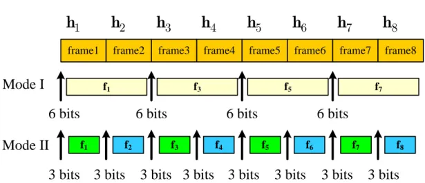
In our work, we have two codebooks F and ₁ F corresponding to 6-bit ₂ quantization and 3-bit quantization at the receiver and the transmitter. For simplicity, we call the mode using the 6-bit codebook for limited feedback as Mode I and the mode using the 3-bit codebook as Mode II. The two modes are defined as follows: (1) Under Mode I scheme, the best precoder is chosen at the receiver, and then the index of the precoder, which is coded in 6 bits, are fed back to the transmitter per two frames; (2) For Mode II, this work is realized per one frame. Therefore, the two modes in our definition have the same feedback rate as 3 bits/time frame.

Instead of using Mode I or Mode II exclusively for the system architecture, we consider a dual-mode scheme in [11], in which two codebooks are available at both

3.1 Dual-Mode Scheme

The dual-mode limited feedback system has two codebooks of different sizes at the receiver and transmitter. In this thesis, we adopt the 3-bit and 6-bit codebooks in the IEEE 802.16e-2005 [10], which have been introduced in Chapter 2. In order to fairly compare between the two modes and select one for use, we consider a fixed-rate feedback scheme as described in [11]. Namely, 6 bits are fed back to the transmitter per two frames in Mode I; 3 bits are fed back to the transmitter per one frame in Mode II. As a result, an equal feedback rate of 3 bits/frame is maintained for each mode. In particular, we assume that the transmitter is able to distinguish between the two modes via feedback bits without extra ones for indicating which mode should be adopted. Also, we assume that the receiver has full knowledge of CSI at the start of each frame so that it can choose the best beamformer and better mode for use in time-varying channel. The dual-mode selection scheme in MISO system is shown in Fig. 3-1

frame1 frame2 frame3 frame4 frame5 frame6 frame7

f1 f3 f5 f7

Mode I

f2

f1 f3 f4 f5 f6 f7 f8

Mode II

6 bits

6 bits

6 bits

6 bits

3 bits

3 bits

3 bits 3 bits

3 bits

3 bits

3 bits

3 bits

frame8

1

h

h

₂

h

₃

h

₄

h

₅

h

₆

h

₇

h

₈

3.2 Throughput-Based Criterion

Before a further discussion, we should first define the throughput used in this work. The throughput is defined as (maximum reliable transmission rate) × (1–bit error rate), whose physical meaning is the number of correct bits per second that can be achieved without any error-control coding if the transmitter use the channel capacity as the transmission rate. The maximum reliable transmission rate is channel capacity ( ) 2 ( ) log 1 C γ = +γ (3.1) where γ is given by (2.2).

The bit error rate (BER) generally has no closed-form solution, therefore we turn to its upper bound from the relation with symbol error rate (SER)

2

SER

BER SER

log M ≤ ≤ . (3.2)

Considering the worst case, we choose SER as BER. Finally the throughput is written as

(

)

( ) ( ) 1 _M( )

T γ =C γ ⋅ −P γ (3.3)

where P γ is the SER for a given modulation scheme, which is M-QAM in our _M( ) case, and has the following formula [19]:

2

3.3 Modal Metric

In order to select a better mode for use at the transmitter, we should first define the modal metric used at the receiver. Modal metric, as implied by its name, is used as a gauge to compare between two modes, and a careful choice of it can increase the system performance. Our modal metric is defined as the average throughput between two consecutive frames:

{

_{, 1,}

}

{ } 1 ( ) [ ( )] , 1,2 2 m Tk m γ Tk+ m γ m Γ = +E ∈ (3.6)

where T_{i j,} ( )γ is the throughput for the i th frame under the j th mode and [ ]⋅E denotes expectation over channel statistics. This type of modal metric is also defined in [11]in which the modal metric is defined as

{

_{, 1,}

}

{ } 1 ( ) [ ( )] , 1,2 2 m SERk m γ SERk+ m γ m Γ = +E ∈ (3.7)

where SER_{i j,} ( )γ is the SER for the i th frame under the j th mode. Therefore, the selection criterion in [11] is called SER-based criterion.

The reason for the expectation is based on the fact that we assume the receiver has full knowledge of channel statistics at k th frame but nothing about it for the coming frame. Taking average over two time frames can help the receiver exploit the information of channel correlation and further enhance the accuracy of our modal metric. If the channel correlation ρ is equal to 1, then there is no need to take the expectation over the (k +1)th frame, so the modal metric in this case becomes

{ }

, ( ) 1,2

m Tk m γ m

3.3.1 Computation of Modal Metric in Mode I

The expected value of the throughput corresponding to Mode I conditioned on

k

h can be formulated as

1,1 ₀ 1,1

[T_k+ ( )]γ =

_∫

∞T_k+ ( )γ ⋅f_Γ(γ h_k) dγ

E (3.9)

where γ = hH_k+1f_ks₊₁2/N₀ and f γ_Γ( h is the probability density function (PDF) _k) of the random variable Γ conditioned on h . In order to compute this integral, we _k need to find out the distribution of Γ .

In this mode, the selected precoder for the (k +1)th frame is the same to that for the previous one, i.e., f_ks₊₁ =f , therefore, we can rewrite γ as _ks hH_k+1f_ks 2/N₀. Furthermore, we transform (3.9) into another representation

1,1 ₀ 0 [T_k ( )] T( y ) f y_Y( _k) dy N γ ∞ + =

∫

⋅ h E (3.10)

where Y = h_kH₊₁f_ks2 and f y h is the PDF of random variable Y conditioned _Y( _k) on h . The derivation of _k f y h can be found in [11] and is illustrated as follows. _Y( _k) Replacing h_{k +1} with ρh_k + Δh in hHk+₁f , we obtain ks

(

) (

)

1

H s

k+ k = mR +jmI + ΔhR + Δj hI

h f (3.11)

( ) ( ) 2 2 ₂ 1 /2 1 /2 1 R I X X Z Y ρ ρ ρ = + = − − − (3.12)

then we find that Z is a noncentral Chi-square distributed random variable with degrees of freedom being 2 and the noncentrality parameter being λ [20]

(

)

( )

( )

( ) 2 2 2 2 1 /2 1 /2 1 R I H s k k m m λ ρ ρ ρ ρ = + = − − − h f . (3.13)

Therefore, the PDF of Y can be directly obtained from Z

( ) ( / ) 1 ( ) Y k Z ( ) Y k Z dF y dF y a y f y f dy dy a a = h = = h (3.14) where 1 2

a = −ρ, and f z is the PDF of random variable Z _Z( )

0 1 ( ) ( ) exp( ) ( ) 2 2 Z z f z = − +λ ⋅I λz . (3.15) 0( )

I i is the modified Bessel function of the first kind of zero order [21]. Finally, The expected value of throughput corresponding to Mode I conditioned on h can be _k written as 1,1 2 2 0 0 0 [ ( )] ( ) 1 2 ( ) exp( ) ( ) 1 1 1 k H s k k _{H s} k k T y y T I y dy N γ ρ ρ ρ ρ ρ + ∞ − + = ⋅ ⋅ − − −

∫

h f h f E (3.16)

The derivation given above is based on the assumption that the channel correlation ρ is not equal to 1, or Equation (3.12) does not make any sense. In this case, when ρ is equal to 1, the channel condition of the k th frame is the same to that of the (k +1)th frame, so the expectation is meaningless and the throughput of the (k + th frame is the same to that of the k th frame. 1)

3.3.2 Computation of Modal Metric in Mode II

The expected value of throughput corresponding to Mode II is much involved than that in Mode I since the best precoder is reselected in the (k +1)th frame. Therefore, we have two uncertainties: hH_{k +1} and f_{k +1}. The formula for the expected value of throughput is formulated in the same way to that under Mode I

1,2 ₀ 1,2

[T_k+ ( )]γ =

_∫

∞T_k+ ( )γ ⋅f_Γ(γ h_k) dγ

E (3.17)

The receive SNR can then be derived as

Γ =SNR⋅ hH_k+1f_ks₊₁2 2 2 2 ₁ 1 1 SNR max i H k k i k + + ∈ ₊ = ⋅ ⋅ f h h f h F = SNR⋅ ⋅ (3.18) U V where U = h_k+1 2, 2 2 1 1 max i H k i k V + ∈ ₊ = f h f h

F . In other words, the receive SNR is a

multiplication of two random variables U and V under the condition that h is _k given.

The derivation of PDF of U conditioned on h is similar to that of Y in _k Mode I, so we omit it here. The result is

2 2

( ) ( u )

bound, thus the resulted expected value is a lower bound, which is questionable to be used as a modal metric in Mode selection. Therefore, in our work, we turn to use V , which is a random variable generated from V with h being averaged out, as our k

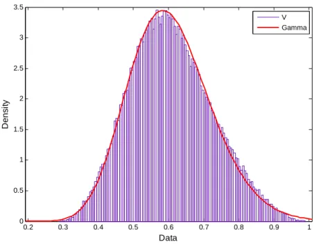
alternative. With the help of numerical experiments, the plot of f v is depicted in _V( ) Fig. 3-2. Then we approximate the PDF of random variable V with Gamma distribution [22, 23]

(

)

[ ) 1exp / ( ) 0, ( ) a a v b f v v v a b − − = ∈ ∞ Γ ⋅ (3.20)

where κ =26.5 and η =0.023. Although the support of gamma distribution lies in

+

, which does not match that of random variable V , we may still regard ( )f v as an approximation of the distribution of V , thus

(

)

_{[ ]} 1exp / ( ) 0,1 ( ) V v f v vκ _κη x κ η − − ≅ ∈ Γ ⋅ (3.21)

To examine the tightness of this approximation, we compare the root mean square error (RMSE) of using the function ( )f v as well as that of using different order of polynomials, and the result is plotted in Fig. 3-3. As we can see, the approximation with ( )f v is tight enough.

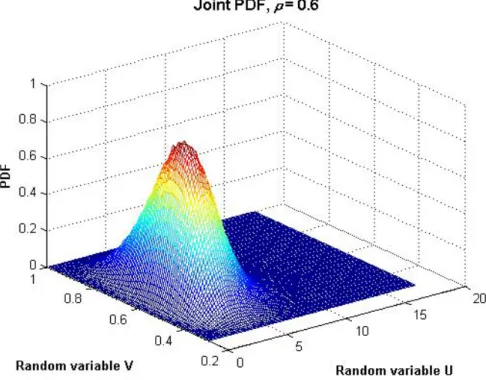
Moreover, two random variables U and V are independent. Instead of giving a proof in detail, we provide an alternative way to demonstrate it. The chief reason for the independence lies in the fact that V has nothing do with h , thus making them _k an independent pair. To better illustrate this, we give the graphs of the jointly distribution of UV and the product of their distributions.

0.2 0.3 0.4 0.5 0.6 0.7 0.8 0.9 1 0 0.5 1 1.5 2 2.5 3 3.5 Data De n s it y V Gamma

Fig. 3-2 Histogram of the random variable V and its approximation with Gamma distribution 0.2 0.4 0.6 0.8 1 1.2 1.4 RMSE Polynomial f(v)

Fig. 3-4 Joint PDF of random variables V and U

3.4 Selection of Good Mode and Beamformer

The rule for selecting a suitable mode and a specific precoder is described as follows: the receiver first determines the mode m for use based on the value of each modal metric, i.e., Mode I is chosen if Γ > Γ and Mode II on the other hand. _{1 2}

(Mode I) if (Mode II) if 1 2 2 1 1 , 2 , m m ⎧ = Γ > Γ ⎪⎪ ⎨⎪ = Γ > Γ ⎪⎩ (3.22)

After choosing the mode type, the receiver chooses the precoder fs maximizing the throughput { } arg max ( ) 1,2 m s _{T γ m} ∈ = ∈ f f F (3.23) and feeds back the index of the precoder to the transmitter. Since ( )T γ is a

monotonically increasing function of γ , (3.23) becomes { } 2 arg max 1,2 k m s H k k m ∈ = ∈ f f h f F (3.24) The rule for selecting a good mode and a beamformer can be better described in the

3.5 Numerical Results

In this section, we shall give some simulations to demonstrate the advantages of the dual-mode scheme and the proposed selection criterion. Table 3-1 lists all parameters in our simulation.

Table 3-1 Simulation parameters

Parameter Value

Channel Rayleigh fading channel

(First-order Markov channel model)

Modulation 16 QAM

Number of transmit antennas 4

Number of receive antennas 1

Fixed average feedback rate 3 bits per frame

Frame length 128 symbols

Number of frames 10000

Codebook

Transmit beamforming codebooks in IEEE 802.16-2005

0.1 0.2 0.3 0.4 0.5 0.6 0.7 0.8 0.9 3.4 3.6 3.8 4 4.2 4.4 4.6 4.8 5 Channel Correlation ρ Thr oughput ( b it s/ s/ H z )

4x1 MISO System, 16 QAM , SNR = 10dB

16QAM (Mode Selection) 16QAM (3-bit Precoding) 16QAM (6-bit Precoding)

Fig. 3-7 Dual-mode scheme and single-mode scheme with SNR = 10dB and 16 QAM

In this figure, we can observe that the dual-mode scheme with the proposed mode selection criterion adequately switch between the other two single-mode schemes, which in our case are the 3-bit precoding scheme and the 6-bit precoding scheme. In low-correlation regime, the receiver prefers Mode II. Due to the rapid fluctuation of channel statistics, the system is able to achieve better performance if it reselects the precoder at the start of each frame. On the other hand, in high-correlation regime, the receiver turns to use Mode I. Because the channel statistics varies slowly, the high resolution of the 6-bit codebook is able to compensate for the performance degradation due to the use of same precoder over two frames.

3.6 Summary

In this chapter, we first introduce the dual-mode scheme in which two different sizes of codebooks are adopted. The goal of using dual-mode scheme is to achieve a better system performance on the premise that adequate selection criterion can be used to switch between the two. Afterwards, we propose our mode selection criterion by first defining the throughput in this work and then the modal metric.

In Section 3.2, we give the definition of the throughput whose physical meaning is the number of correct bits per second that can be achieved without any error-control coding if the transmitter use the channel capacity as the transmission rate. In Section 3.3, the definition of the modal metric is given. The modal metric is able to exploit the channel correlation between the consecutive two frames by taking average of the throughputs corresponding to each mode under the assumption that the receiver has full knowledge CSI. In particular, the modal metric involves the expectation of the throughput pertaining to the next frame since the receiver has no idea about the exact channel condition of it. The detailed analysis of modal metric corresponding to Mode I and Mode II is also derived. Then in Section 3.4, we describe the selection rule for the good mode and the precoder. Finally, a simulation is given to justify the proposed algorithm for the dual-mode scheme.

Chapter 4

Modal Metric Approximation

In Chapter 3, the definition and derivation of the modal metric corresponding to Mode I and Mode II are given; moreover, simulations justify the utility of the modal metric by showing that the dual-mode scheme outperforms the single-mode scheme over full range of channel correlations. The superior performance is ascribed to the consideration of channel correlation in the modal metric. Namely, the expected value of throughput of the coming frame is considered when performing the mode selection. While the expected value of the throughput with respect to Mode I and Mode II are derived in Chapter 3, the integral are a little bit troublesome when performing this algorithm in practical, and to simply the computation of this integral is one of the future works in [11]. Therefore, we wonder if there are closed-form solutions for them. Unfortunately, to our best knowledge, due to the combination of the various difficult-analyzing functions in the integrals, the answer is no. To seek what is less

4.1 Approximation of Modal Metric in Mode I

We start the approximation with the equation (3.10) and assume that ρ ≠ . 1 Since (3.10) can be rewritten as

0 0 1 ( y ) _Z( ) y T f dy N a a ∞ ⋅

∫

. (4.1)

We first analyze f y a a . Recall that _Z( / )/ a =(1−ρ)/ 2 and

0 1 ( ) ( ) exp( ) ( ) 2 2 Z z f z = − +λ ⋅I λz (4.2) where 2 2 1 H s k k λ ρ ρ = − h f (4.3) therefore 2 2 0 2 2 ( ) 1 1 1 1 2 2 ( ) exp( ) ( ) 1 2 1 1 H s k k H s Z k k y y y f I a a ρ ρ ρ ρ ρ ρ ρ − + − − = ⋅ − − − h f h f ₁

(

, 2

)

exp( ) ₀( 2 2) 1 1 H s H s k k k k y R ρ I ρy ρ ρ − = ⋅ ⋅ − − h f h f (4.4) where

(

2

)

2 1 1 , exp( ) 1 1 H s k k H s k k R ρ ρ ρ ρ − = − − h f h f (4.5) Therefore (4.1) turns to

(

2

)

1 0 0 2 2 0 0 0 2 0 1 ( ) ( ) , 1 3 log 1 1 2 1 1 2 exp( ) ( ) 1 1 H s Z k k H s k k y y T f dy R N a a y y Q N M M N _dy y I y ρ ρ ρ ρ ∞ ∞ ⋅ = ⎡ _{⎛ ⎞ ⎛ ⎛ ⎞ ⎛ ⎞⎞} ⎤ ⎢ ⎜⎜ + ⎟⎟⋅ −⎜⎜ ⎜ − ⎟ ⎜⎜ ⎟⎟⎟⎟ ⋅⎥ ⎢ ⎜⎜ ⎟⎟ ⎜⎜ ⎜⎜⎝ ⎟⎟⎠ ⎜⎜ − ⎟⎟⎟⎟⎟ ⎥ ⎢ ⎝ ⎠ ⎝ ⎝ ⎠⎠ ⎥ ⋅ _{⎢ ⎥} ⎢ ₋ ⎥ ⎢ _⋅ ⎥ ⎢ _{− −} ⎥ ⎣ ⎦

∫

∫

h f h f (4.6)

Since Q-function has no closed form representation, we turn to its approximation [24]:

2 2 1 1 2 ( ) exp exp 12 2 4 3 x x Q x ≅ ⎜_⎜⎜⎜⎛− _⎟⎞_⎟⎟⎟+ ⎜_⎜⎛⎜_⎜− _⎟⎞⎟_⎟⎟ ⎝ ⎠ ⎝ ⎠ (4.7)

With this approximation,

( ) 2 0 2 0 0 1 3 1 2 1 1 1 1 3 1 2 1 2 1 exp exp 12 2 1 4 1 y Q M M N y y M M N M N ⎛ _{⎛ ⎞} ⎛ ⎞⎞_⎟ ⎜ _{⎜ ⎟} ⎜ ⎟_⎟⎟ ⎜ − _⎜ − _⎟ ⎜ _⎟⎟ ⎜ ⎜⎝ ⎟⎠ ⎜⎜ ⎟⎟ ⎜ _⎝ − _⎠⎟ ⎝ ⎠ ⎛ _{⎛ ⎞}⎡ ⎛ ⎞ ⎛ ⎞⎤⎞_⎟ ⎜ ⎜ ⎟⎢ ⎜ ⎟ ⎜ ⎟⎥⎟ ⎜ ⎟ ⎟ =⎜⎜⎝⎜ − ⎜⎝⎜ − ⎟⎠⎟ ⎢_⎣⎢ ⎝⎜⎜⎜− − ⎠⎟⎟+ ⎜⎜⎝⎜− − ⎟⎠⎟⎥⎥_⎦⎟⎟⎠⎟ ( ) ( ) ( ) 0 0 0 0 0 1 3 1 2 1 exp exp 3 2 1 1 1 3 1 7 exp exp 144 1 24 2 1 2 1 4 1 4 exp 16 1 M y M y M M N M M N y y M N M N M M M _y M N ⎛ ⎞ ⎛ ⎞ − _{⎜ ⎟⎟} − _{⎜ ⎟⎟} = − ⎜_⎜⎜− _⎟⎟− ⎜_⎜⎜− _⎟⎟ − ⎝ − ⎠ ⎝ ⎠ ⎡ ⎛_⎜ ⎞_⎟ ⎛_⎜ ⎞_⎟⎤ ⎢ _{⎜− ⎟⎟+ ⎜− ⎟⎟}⎥ ⎢ ⎜⎜ ⎟ ⎜⎜ ⎟⎥ ⎛ − + ⎞_⎟⎢ ⎝ − ⎠ ⎝ − ⎠_⎥ ⎜ _⎟ + ⎜_{⎜⎜ ⎟⎟⎢ ⎥} ⎛ ⎞ ⎝ ⎠ ⎢ _{⎜ ⎟} ⎥ ⎟ + − ⎢ ⎜_{⎜⎜ ⎟⎟} ⎥ ⎢ ⎝ − ⎠ ⎥ ⎣ ⎦ (4.8)

Denote by E(α β the integral , )

(

2

)

1 2 2 0 0 0 0 , 2

log 1 exp exp( ) ( )

1 1 H s k k H s k k R y y y I y dy N N ρ α β ρ ρ ρ ∞ ⋅ ⎡ ⎛_⎜ ⎞_⎟ ⎛_⎜ ⎞_{⎟ −} ⎤ ⎢ _{⎜ + ⎟⎟⋅ ⎜− ⎟⎟⋅ ⋅} ⎥ ⎢ ⎜⎜⎝ ⎟⎠ ⎜⎜⎝ ⎟⎠ − − ⎥ ⎣ ⎦

∫

h f h f (4.9) Equation (4.6) turns to ( ) ( ) ( ) ( ) 1 3 1, 0 , 3 2 1 1 2 1 2 1 3 , , 1 36 1 1 2 1 7 1 2 1 4 , , 6 2 1 4 1 M E E M M M M M E E M M M M M M M M E E M M M M ⎡ _{⎛ − ⎞} ⎤ ⎟ ⎢ _{− ⎜}⎜ _⎟ ⎥ ⎟ ⎢ _{⎜⎜⎝ − ⎟⎠} ⎥ ⎢ ⎥ ⎢ _{⎛ ⎞} ⎥ ⎢ ⎛_{⎜ −} ⎞_{⎟ ⎜} ⎛_{⎜ − +} ⎞_{⎟ ⎟} ⎥ ⎢− ⎜_⎜ ⎟_⎟+ ⎜_⎜ ⎜_⎜ ⎟_⎟ ⎟_⎟ ⎥ ⎢ ⎜⎝ − ⎟⎠ ⎝⎜ ⎜⎝ ⎠⎟ − ⎟⎟⎠ ⎥ ⎢ ⎢ _{⎛ ⎛ ⎞ ⎞ ⎛ ⎛ ⎞ ⎞} ⎢ _{⎜ ⎜} − + _{⎟⎟ ⎟⎟ ⎜ ⎜} − + _{⎟⎟ ⎟⎟} ⎢+ ⎜_{⎜ ⎜}⎜_{⎜ ⎟⎟ ⎟⎟⎟}+ _⎜⎜ _⎜⎜_{⎜ ⎟⎟ ⎟⎟⎟} ⎢ ⎜⎝ ⎝ ⎠ − ⎠ ⎜⎝ ⎝ ⎠ − ⎠ ⎥ ⎥ ⎥ ⎥ ⎥ .(4.10)

fitting [25]: 7 2 0 0 log 1 n [0,20] n n y a y y N ₌ ⎛ _⎞⎟ ⎜ _{+ ⎟≅ ∈} ⎜ _⎟ ⎜ _⎟ ⎜⎝ ⎠

∑

. (4.11) Therefore, (4.9) becomes ( ) ₁

(

2

)

7 ₂ 0 0 0 0 , , 1 2 exp ( ) 1 1 H s k k n H s n k k n E R a y y I y dy N α β ρ β α ρ ρ ρ ∞ = ≅ ⎛ ⎛ _{⎞ ⎟}⎞ ⎜ ⎜ ⎟_{⎟ ⎟} ⋅ ⎜ ⎜_{⎜ ⎜}−_⎜ + _{⎟⎟ ⎟⎟}⋅ ⎜ ⎝ − ⎠ − ⎝ ⎠

∑ ∫

h f h f . (4.12)

Let y=yρ h fH s_{k k} 2, then

( ) ₁

(

2

)

7 _{2( 1)} 1 0 0 2 0 0 , , 1 2 exp ( ) 1 1 H s n k k _{n H s} n n _{k k} H s k k a E R y I y dy N α β α ρ ρ β ρ _ρ ρ + + = ∞ ≅ ⋅ ⎛ _{⎛ ⎞ ⎞⎟} ⎜ _⎟ ⎜ ⎜ ⎟_{⎟ ⎟} ⋅ ⎜ ⎜_{⎜ ⎜}−_⎜ + _{⎟⎟ ⎟⎟}⋅ − − ⎜ ⎝ ⎠ _⎟⎟ ⎜⎝ ⎠

∑

∫

h f h f h f (4.13)

At this point, Let us postpone the computation of this integral for a moment and consider the following lemmas in [21]:

Lemma 1 ( ) ( ) 1 2 2 0 2 2 1 , exp (2 ) 1 1 2 _{exp Re 0} 2 1 2 2 a b a a b x Ax I B x dx a b B B B A M a b b A A − ∞ − − − − ⎛ _⎞⎟ ⎜ Γ_{⎜⎝ + + ⎟⎟⎠ ⎛ ⎞ ⎛ ⎞ ⎛ ⎞} ⎟ ⎟ ⎜ ⎟ ⎜ ⎟ ⎜ ⎟ = _{Γ +} ⎜_⎝⎜⎜ ⎟_⎠⎟ _⎝⎜⎜⎜ ⎟⎟_⎠ ⎝⎜⎜ + + ⎠⎟⎟>

∫

(4.14)

where M_{a b,} ( )⋅ is Whittaker function [21]. Lemma 2 1 2 , 1 ( ) exp( ) ,2 1; 2 2 b a b x M x =x + − Φ − +_⎜⎝⎜⎜⎛b a b+ x⎞⎟_⎟⎟⎠ (4.15) ( )

Φ ⋅ is confluent hypergeometric function [21]. With Lemma 1 and Lemma 2, (4.13) becomes

( )

(

)

( ) ( ) 2 1 2 7 1 0 , , 1 1,1; H s k k n n n E R B a n C n A α β α ρ − + = ≅ ⎛ _⎞⎟ ⎜ _⎟ ⋅ ⋅ Γ + Φ⎜_⎜⎜⎝ + _⎟⎟ ⎠

∑

h f (4.16) where ₂ 0 1 1 1 H s k k A N β ρ _ρ ⎛ _⎞⎟ ⎜ _⎟ =⎜_⎜⎜ + _⎟⎟⋅ − ⎝ ⎠ _{h f} , 0 1 1 C N β ρ ⎛ _⎞⎟ ⎜ _⎟ =⎜_⎜⎜ + _⎟⎟ − ⎝ ⎠ and 1 1 B ρ = − .

To compute Φ

(

n+1,1;B2/A

)

, we again use the following lemmas in [21]: Lemma 3 (p p x, ; ) ex Φ = (4.17) Lemma 4 ( , ; ) ( 2 2 ) ( 1, ; ) ( 1) ( 2, ; ) 1 1 x p q q p p q x p q x p q x p p + − − − + Φ = Φ − + Φ − − − (4.18) Lemma 5 ( ) ( )( ) ( )

(

)

1 1 2 2 2 1 , 2 2 1 2 2 2 b x _n n b x n n b b x e d M x x e b b b n dx − + − + + = + + + (4.19) with n =0,1,2,… and 2b ≠ − − − … 1, 2, 3, Lemma 6 ( ) ( ) ( ) 1 2 1 2 , , b b a b a b x− −M x = −x − − M₋ − (4.20) x with 2b ≠ − − − … 1, 2, 3,

4.2 Approximation of Modal Metric in Mode II

Assuming ρ ≠ and putting (3.21) and (3.19) into (3.17), we obtain 1

(

)

1,2 1 ₁ 0 0 [ ( )] exp / 1 (SNR ) ( | , ) ( ) k W k u v T v u T uv f v dv du a a κ κ γ η ρ κ η + ∞ ₋ = = ≅ − ⋅ ⋅ ⋅ Γ ⋅

∫ ∫

h E (4.24) where κ =26.5,η =0.023, and a =(1−ρ)/ 2. For simplicity, we denote (4.24) as

( ) 0 u H u du ∞ =

∫

(4.25) where ( ) 1 1

(

)

0 exp / 1 (SNR ) ( | , ) ( ) W k v v u H u T uv f v dv a a κ κ η ρ κ η − = − = ⋅ ⋅ ⋅ Γ ⋅

∫

h (4.26)

Since the random variable W is noncentral chi-square distributed with 2N _t degrees of freedom and the non-centrality parameter λ being 2ρ h_k 2/(1−ρ), (4.26) can then be rewritten as

( )

(

)

(

)

1 2 ₂ 2 1 2 ₂ 1 2 2 1 2 0 0 0 1 1 , , exp( ) ( ) ( ) 1 2 1 ( ) ( ) 1 1 3 log 1 1 2 1 1 exp / t t t N k t N N k k v u H u R N u I u uv uv Q N M M N dv v v κ κ ρ κ η ρ ρ ρ ρ η − − − = − − = ⋅ ⋅ ⋅ Γ ⋅ − ⋅ ⋅ − ⎡ _{⎛ ⎞ ⎛ ⎛ ⎞ ⎛ ⎞⎞} ⎤ ⎢ ⎜⎜ + ⎟⎟⋅ −⎜⎜ ⎜ − ⎟ ⎜⎜ ⎟⎟⎟⎟ ⎥ ⎢ ⎜⎜ ⎟⎟ ⎜⎜ ⎜⎜⎝ ⎟⎟⎠ ⎜⎜ − ⎟⎟⎟⎟⎟ ⎥ ⎢ ⎝ ⎠ ⎥ ⋅ _⎢ ⎝ ⎝ ⎠⎠ _⎥ ⎢_{⋅ −} ⎥ ⎢ ⎥ ⎣ ⎦

∫

h h h (4.27) where

(

2

)

2 2 ( ) 1 , , exp( ) 1 1 k k t R ρ N ρ ρ ρ − = − − h h (4.28)

Again, we use the approximation in (4.7) for Q-function, so ( )

(

)

( ) ( ) ( ) 1 2 ₂ 2 1 2 ₂ 1 2 , , exp( ) ( ) 1 2 1 ( ) ( ) 1 1 3 1 2 ,1, 0 , , , , 3 2 1 1 1 2 1 3 , , 36 1 1 2 1 7 , , 6 2 1 t t t N k t N N k k H u u R N u I u M M D u D u D u M M M M M M D u M M M M D u M M ρ ρ ρ ρ ρ − − − ≅ − ⋅ ⋅ − ⋅ ⋅ − ⎛ ₋ ⎞_⎟ ⎛ ₋ ⎞_⎟ ⎜ _⎟ ⎜ _⎟ − ⎜_{⎜⎜ ⎟⎟}− ⎜_{⎜⎜ ⎟⎟} − ⎝ − ⎠ ⎝ ⎠ ⎛ ⎛ _{− +} ⎞ ⎞_⎟ ⎜ ⎜ ⎟_{⎟ ⎟} + ⎜_⎜⎜ ⎜_{⎜⎜ ⎟⎟ ⎟⎟⎟} − ⎝ ⎠ ⎝ ⎠ ⋅ ⎛ ⎛ _{− +} ⎞ ⎜ ⎜ ⎟_⎟ + ⎜_{⎜⎜ ⎟⎟} − ⎝ ⎠ ⎝ h h h 1 2 1 4 , , 4 1 M M D u M M ⎡ ⎤ ⎢ ⎥ ⎢ ⎥ ⎢ ⎥ ⎢ ⎥ ⎢ ⎥ ⎢ ⎥ ⎢ ⎥ ⎢ ⎥ ⎢ _⎞ ⎥ ⎢ _{⎜ ⎟⎟} ⎥ ⎢ _{⎜⎜ ⎟⎟⎟} ⎥ ⎢ ⎠ ⎥ ⎢ ⎥ ⎢ _{⎛ ⎛ − + ⎞ ⎞} ⎥ ⎟ ⎢_{⎢+ ⎜}⎜ ⎜_⎜ ⎟_{⎟ ⎟⎟} ⎥_⎥ ⎟ ⎜ ⎜⎜ ⎟ ⎟⎟ ⎜ ⎝ ⎠ − ⎝ ⎠ ⎢ ⎥ ⎣ ⎦ (4.29) where ( )

(

)

1 ₁ 2 0 0 0 , , 1

log 1 exp exp /

( ) v D u uv uv v v dv N N κ κ α β α β η κ η − = ⎡ ⎛_⎜ ⎞_⎟ ⎛_⎜ ⎞_⎟ ⎤ ⎢ _{⎟ ⎟} ⎥ = ⋅ _{⎢ ⎜⎜}⎜ + _⎟⎟⋅ ⎜_⎜⎜− _⎟⎟⋅ − _⎥ Γ ⋅

∫

_⎣ ⎝ ⎠ ⎝ ⎠ _⎦ . (4.30)

With numerical experiment, we find that H u decays very fast and is negligible for ( )

20

x > , so we approximate D u α β with a polynomial ( , , )( , , ) f u α β using least squares fitting [25]: 7 0 ( , , ) _n n [0,20] n f u α β a u u = =

∑

∈ . (4.31) Denote F(α β by , )

( ) 1,2 [ ( )] 1 3 1 2 1, 0 , , 3 2( 1) 1 1 2 1 3 1 2 1 7 , , 36 1 6 2( 1) 1 2 1 4 , 4 1 k T M M F F F M M M M M M M M F F M M M M M M F M M γ + ≅ ⎛ _{− ⎟}⎞ ⎛ ₋ ⎞_⎟ ⎜ _⎟ ⎜ _⎟ − ⎜_{⎜⎜ ⎟⎟}− ⎜_{⎜⎜ ⎟⎟} − − ⎝ ⎠ ⎝ ⎠ ⎛ ⎛ _{− +} ⎞ ⎞_⎟ ⎛ ⎛ _{− +} ⎞ ⎞_⎟ ⎜ ⎜ ⎟_{⎟ ⎟} ⎜ ⎜ ⎟_{⎟ ⎟} + _⎜⎜ _⎜⎜_{⎜ ⎟⎟ ⎟⎟}+ _⎜⎜ _⎜⎜_{⎜ ⎟⎟ ⎟⎟} ⎟ ⎟ ⎜ ⎝ ⎠ − ⎜ ⎝ ⎠ − ⎝ ⎠ ⎝ ⎠ ⎛ ⎛ _{− +} ⎞ ⎞_⎟ ⎜ ⎜ ⎟_{⎟ ⎟} + ⎜ ⎜_{⎜ ⎜⎜ ⎟⎟ ⎟⎟⎟} ⎜ ⎝ ⎠ − ⎝ ⎠ E (4.33)

The computation for F(α β is similar to that for (4.12), and the result is , )

( )

(

)

( )

2 2 7 0 ( ) , exp( ) 1 , ; k t n n t t n t F N n B a B N n N N A ρ α β ρ − = − = − ⎡ Γ + ⎛_⎜ ⎞_⎟⎤ ⎢ _⎥⎟ ⋅_⎢ Φ⎜_⎜⎜ + _⎟⎟⎥ Γ ⎝ ⎠ ⎢ ⎥ ⎣

∑

⎦ h (4.34) where ( ) 2 1 1 _k A ρ ρ = − h , and 1 1 B ρ =

− . The closed form representation for

( )

4.3 Numerical Results

In this section, we give some simulation results to demonstrate the effectiveness of the throughput-based criterion. For the sake of simplicity, we denote E[T_k+1,1( )]γ as T ; approximated ₁ E[T_k+1,1( )]γ as T ; ₁* E[T_k+1,2( )]γ as T ; approximated ₂

1,2

[T_k+ ( )]γ

E as T . Moreover, the throughput performance with respect to the ₂* dual-mode scheme, the single-mode scheme with 3-bit precodeing, and the single-mode scheme with 6-bit precoding are also given. Finally the proposed mode selection criterion is compared with other criteria. Table 4-1 lists all parameters in our simulations.

Table 4-1 Simulation parameters

Parameter Value

Channel Rayleigh fading channel

(First-order Markov channel model)

Modulation 16QAM, 64 QAM

Number of transmit antennas 4

Number of receive antennas 1

Fixed average feedback rate 3 bits per frame

Frame length 128 symbols

4.3.1 Approximation vs. Exact Value (Mode I)

Fig. 4-1 shows the expected value of throughput over the (k +1)th frame under Mode I with 16-QAM modulation. Three different channel correlations: ρ =0.1,

0.5

ρ = , and ρ =0.9 are considered. First, the expected value of the throughput over the (k +1)th frame is an increasing function of SNR. Second, As the channel correlation gets larger, the performance gets better. The reason is that the best precoder for beamforming over the k th frame is near optimal for the (k +1)th frame. Moreover, the approximation of the expected value is shown to be very tight for different channel correlations and SNRs. The proposed approximation is also shown to be very tight for different modulations in Fig. 4-2

0 2 4 6 8 10 12 14 16 0 1 2 3 4 5 6 7 SNR (dB) E [Thr o ughput ] ( b it s/ s/ H z )

4x1 MISO System, 16 QAM 6-bits precoding

ρ = 0.9 ρ = 0.9 (Approximation) ρ = 0.5 ρ = 0.5 (Approximation) ρ = 0.1 ρ = 0.1 (Approximation)

0 2 4 6 8 10 12 14 16 0 1 2 3 4 5 6 7 SNR E [Thr oughput ] ( b it s/ s/ H z )

4x1 MISO System, 64 QAM 6-bits precoding

ρ = 0.9 ρ = 0.9 (Approximation) ρ = 0.5 ρ = 0.5 (Approximation) ρ = 0.1 ρ = 0.1 (Approximation)

Fig. 4-2 T vs. ₁ T with 64 QAM and different channel correlations ₁*

4.3.2 Approximation vs. Exact Value (Mode II)

Fig. 4-3 shows the expected value of throughput over the (k +1)th frame under Mode II with 16-QAM modulation. Three different channel correlations: ρ =0.1,

0.5

ρ = , and ρ =0.9 are considered. First, the expected value of the throughput over the (k +1)th frame is an increasing function of SNR. Second, we can observe that unlike Mode I, in which the performance gets better as the channel correlation gets larger, the performance corresponding to different channel correlations are almost the same. The reason is that the best precoder for beamforming over the k th frame is

0 2 4 6 8 10 12 14 16 0 1 2 3 4 5 6 7 SNR (dB) E [T hr oughput ] ( bi ts /s/ H z )

4x1 MISO System, 16 QAM 3-bit precoding

ρ = 0.9 ρ = 0.9 (Approximation) ρ = 0.5 ρ = 0.5 (Approximation) ρ = 0.1 ρ = 0.1 (Approximation)

Fig. 4-3 T vs. ₂ T with 16 QAM and different channel correlations ₂*

0 2 4 6 8 10 12 14 16 0 1 2 3 4 5 6 SNR (dB) E[ T hr oughput ] ( bi ts/ s /H z )

4x1 MISO System, 64 QAM 3-bit precoding

ρ = 0.9 ρ = 0.9 (Approximation) ρ = 0.5 ρ = 0.5 (Approximation) ρ = 0.1 ρ = 0.1 (Approximation)

4.3.3 Dual-Mode Scheme vs. Single-Mode Scheme

To better examine the improvement of the dual-mode scheme over the single-mode scheme, average throughput over different channel correlations at a fixed transmit SNR is compared. In Fig. 4-5 and Fig. 4-6, each figure has four lines corresponding to the single-mode schemes with 3-bit and 6-bit codebook respectively, the dual-mode scheme using exact modal metric, and the dual-mode scheme using the approximated modal metric.

In each figure, we can see that the system performance does not remain well in all channel correlations using Mode I or Mode II exclusively. Mode I is good at low channel correlations since the receiver selects the best precoder at each time frame. While at high channel correlations, Mode II works better since the high resolution of the codebook compensates for the loss caused by choosing precoder seldom. Finally, the proposed algorithm of model selection works well for the dual-mode scheme which outperforms each single-mode scheme in full range of channel correlations because it always selects a better mode for use. Moreover, the proposed approximation for the modal metric is very tight over different channel correlations and modulations.

0.1 0.2 0.3 0.4 0.5 0.6 0.7 0.8 0.9 3.4 3.6 3.8 4 4.2 4.4 4.6 4.8 Channel Correlation ρ T hr oughput ( bi ts /s/ H z )

4x1 MISO System, 16 QAM , SNR = 10dB

16QAM (Mode Selection) 16QAM (Mode Selection App) 16QAM (3-bit Precoding) 16QAM (6-bit Precoding)

Fig. 4-5 Dual-mode scheme, Dual-mode scheme with approximated modal metric and single-mode scheme with SNR = 10dB and 16 QAM

0.1 0.2 0.3 0.4 0.5 0.6 0.7 0.8 0.9 2.1 2.2 2.3 2.4 2.5 2.6 2.7 2.8 2.9 3 Channel Correlation ρ Thr o ughput ( b it s /s /H z )

4x1 MISO System, 64 QAM , SNR = 10dB

64QAM (Mode Selection) 64QAM (Mode Selection App) 64QAM (3-bit Precoding) 64QAM (6-bit Precoding)

Fig. 4-6 Dual-mode scheme, Dual-mode scheme with approximated modal metric and single-mode scheme with SNR = 10dB and 64 QAM