REDUNDANCY DESIGN FOR A FAULT TOLERANT SYSTOLIC ARRAY

(1)

Redundancy design for a fault tolerant systolic

array

J.-J. Wang C.-W. Jen

Indexing term: Array processing

Abstract: A systematic design methodology for redundant systolic arrays is proposed. Redundancies consisting of space-shift, time-shift and space-time-shift schemes are applied suc- cessfully to detect or mask permanent faults, transient faults or both. Various redundancy designs for different utilisation efficiencies of processor elements can be obtained at the design stage by a dependent graph and its associated algebraic transformation. A customised optimal redundant systolic array design can be achieved for various performance requirements, including throughput rate, latency, average computation time, hardware cost and capabilities of fault detection and fault masking.

1 Introduction

A systolic array [l] is a computing network that is composed of many processor elements (PES) and local inter- connections between them. It maximises computation concurrences, including multiple processing and pipeline processing; it is therefore suitable for the computation- intensive problems existing frequently in image and digital-signal processing. However, a major difficulty with such high degrees of integration is that a single flaw in a PE will lead to an erroneous result and render the entire array useless. Therefore, fault-tolerance techniques must be incorporated.

Various fault-tolerance techniques on systolic arrays, such as static redundancy and dynamic reconfiguration, have been proposed [2-131. For conventional static redundancy, three techniques can be applied : fault detection (duplication and RESO [3]), fault masking (TMR) and algorithm-based fault tolerance [4, 51. RESO is useful for detecting transient faults in PE, but strictly it causes time redundancy. Algorithm-based fault tolerance has the advantages of lower hardware and time overheads, but the drawbacks of algorithm-specific design and arithmetic errors, including truncations and over- flows.

In general, replicated computation in a systolic array can repeat the P E processing and then make a matching or voting test, which is a recognised, effective means of concurrent error detection or masking in real-time fault tolerance applications [9, lo]. Duplication, TMR or time redundancy at P E level all belong to this class. The design objective is to maximise the fault coverages while

Paper 7138E (C2, C3), first received 7th October 1988 and in revised form 25th September 1989

The authors are with the Institute of Electronics, National Chiao Tung University, 75 Po-Ai St., Hsinchu, Taiwan, Republic of China 218

minimising the corresponding hardware and time overheads.

Transient faults and permanent faults both occur in real-time environments. For detecting purpose, a permanent fault can be resolved by comparing the computing results from different PES assuming that only single fault exists in systolic array. A transient fault can be detected by comparing the results from same P E at a different time. Of course, comparison of results from different PES executed at different times will detect both permanent and transient faults. Therefore, the replicated computation techniques working on array structure can be summarised into three operating modes : space-shift, time-shift and space-time-shift, as shown in Table 1. The enhanced RESO technique [ l l , 123 is one specific design example. In this paper, a systematic and more generalised redundant design approach for systolic array is provided. Table 1 : Three operating modes of the replicated computa- tion in space-time domain

operating modes space-shift

I

time-shift

k

s p a c e - t i m e - s h i f t I f a u l t detected structure permanent fault PE12

i

transient fault

I

permanent fault and

I

transient fault The systolic array can be characterised by the following attributes [14] : (1) synchronicity, (2) regularity and modularity, (3) spatial and temporal locality and (4)

pipelinability. Regular, modular design and spatial locality will improve space-shift, while synchrony and temporal locality will benefit time-shift. Pipeline design gives the system high throughput rate, but the PES often lie idle in some nonfull pipelining cases. Nonfull pipeline often occurs because of the synchronous systolisation or limited input/output bandwidth [l5, 161. These idle PES can be seen as the pseudohardware to be used for redundancies. Hence the effective redundancy design in systolic arrays is a kind of space-time management problem. And, as we know, the synthesis procedure of a systolic array can be seen as a space-time transformation. Therefore it will be the most effective to consider redundancies in design stage for a systolic array.

(2)

2

In this Section, a systematic design method for a systolic array is introduced. It is a two-step procedure. The first step is to construct a dependence graph from the algorithm expression. The dependence graph approach is an effective way to maximise the parallelisms in temporal and spatial domains [14]. The second step is a space- time transformation from the dependence graph to a systolic array.

2.1 Dependence graph

The dependence graph (in short DG) is the 'unrolling' of an algorithm, which exposes the inherent data dependencies so that the concurrences can be easily extracted. The D G can be easily constructed from an indexed and localised single assignment form of an algorithm expression. The formal definition can be described as

Design methodology f o r a systolic array

Dejinition 1 : A dependence graph is a directed graph composed of nodes and directed arcs. Nodes locate at some index points in n-dimensional index space, and each node associates with a function whose operands reside in incoming arcs while the computing results reside in out- going arcs. Therefore, the directed arcs represent the data flow dependencies. The D G can be expressed as an algebraic structure

DG = ( J " , D), where

J" is the set of triples ( j , cj,fj), where j is an index point from a finite integer set Z", c j is the function associated with the index point a n d & is the set of data associated with the index point j .

D is the set of triples ( d , e(d),f,), where d is the data- dependent vector in n-dimensional index space and e(d)

the data-dependent edges or arcs in the graph along the direction specified by d . f , is the set of data associated with e(d).

2.2 Space-time transformation

Given a DG, a systolic array can be derived by a linear transformation. This transformation matrix, which maps the D G into a systolic array can be expressed as

where the 1 x n vector W , termed the time-schedule func- tion, maps the index space into time sequence, and the (n - 1) x n submatrix S , termed the space-transformation function, maps n-dimensional index space into an ( n - 1)- dimensional systolic array. This transformation T , com- prising time schedule and node assignment to array space, is sometimes called the space-time transformation.

To determine W and S , we first have to choose arbi- trarily a projection direction Pd on the DG. The space- transformation function S can be obtained by the chosen P d

[SI.

For correct timing scheduling, W has to obey the following conditions :

(1) W

.

d i 2 1 for any dependent vector di on the DG.

(2)

w

' P d # 0.

If W and S are determined through this space-time trans- formation T , a systolic array can be derived. The systolic array can be abstracted by a model defined as follows: Dejinition 2: A systolic array model can be expressed as a structure S A = ( I " - ' , L ) where: I n - ' is the set of triples (i,

C i ,

Fi), where i is the index point in ( n - 1) dimension

space where PE is located.

C i

and F i are the function and the set of data streams associated with the index point i.

L is the set of triples ( I , De(l), F',), where 1 is the physi- cal directed links connected between processors. De(l) is the delay elements on the physical directed link 1. F , is the set of data streams associated with the physical directed link 1.

The PE space and physical directed link of a systolic array are therefore easily obtained by:

(1) Node transformarion: an index point j E J" (index in DG) is mapped by

which means that the index point j is executed in index point io') of the corresponding I n - ' PE space in systolic array at time to').

(2) Link transformation: a data-dependent vector d in D G is mapped to a physical directed link

The 1 is a physical directed link in systolic array and De(l) is the delay associated with the link 1. Actually, the number of extra delay units inserted between PES is

One important performance parameter for the designed systolic array is the pipeline period a, which is the time interval in clock units between two successive input data. It also indicates the time interval between two successive activities of a processor. By our transformation, U = W .

p d . a = 1 means that the processor is busy in every clock and U = 2 means the processor is activated in every other clock, i.e. busy and idle alternately.

Taking an example of band matrix-vector multiplica- tion, D G is shown in Fig. l a while two array designs (De([) - 1).

a l l 0 0 0 0

b

a Dependence graph for band matrix-vector multiplication

b Systolic array with pipelining period a = 1

c a = 2

Fig. 1

(3)

which are projected along two projection directions [0, 11 and [l, 11 are shown in Figs. l b and c, respectively. In these designs, time schedule function W is selected as

[I, 11. For [0, I] projection, S = [I, 01, then c1 = 1 is obtained. For [l, 11 diagonal projection, S = [l, - 11, U

is 2 and so the data throughput rate and the utilisation efficiency of processor would be halved.

2.3 Pipeline period scaling and delay transfer As described in Section 2.2, various transformations may be found by choosing different projection directions, which will result in different designs. Meanwhile, some rules may be applied on the algebraic transformation matrix to get new transformations, which will be useful for fault-tolerant systolic array design.

2.3.1 Pipeline period scaling: If a new transformation

obtained by the time schedule function is multiplied by a positive integer k , i.e. wk= kW, this is termed pipeline

period scaling. For this new transformation, not only U

but also delay elements on the links have to be scaled up by a factor of

k.

Incidentally, the PE is idle more frequently and more delay elements are needed. Therefore, a time schedule function wkis called a scaled time-schedule

function if it can be described by wk= k

.

W where k is a positive integer.

2.3.2 Delay transfer: Given any cutset that partitions a

systolic array into two parts, we can group the edges of the cutset into two sets: inbound and outbound edges. As

we know, on systolisation [13], the advancing

k

time units on all the outbound edges would pause k time units on the inbound edges, or vice versa. This procedure of delay transfer can be described mathematically by

T , . D =

_ _ _ _ _

m_ _ _ _ _ _ _ . D f o r m = 1 , 2

,...,

n - 1

["

+

","-.

where s, is any row vector of S and h, is any integer. The new transformation

T,

is obtained by transferring

h,

.

s,

.

di

delay time units to each directed link

li.

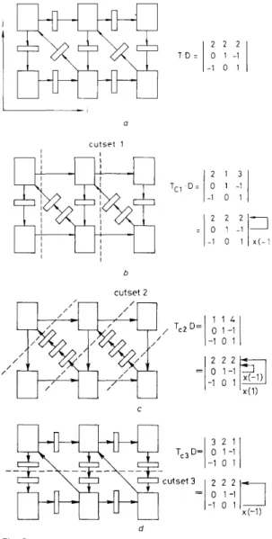
Two examples follow. Fig. 2a is a systolic array design as shown in Fig. l b for band matrix-vector multiplication in which the corresponding transformation is described by T . D. The first element of each column in T

.

D rep- resents the delay element De(Z) in each directed link 1. The other elements represent the existing direction of 1. In

+EEEE

T O = )

::I

J b 3 )

=

1;

1)

a cutset b Fig. 2

a Systolic array for band matrix-vector multiplication b Delay transfer for systolic array

Fig. 2a, there are (De(l) - 1) delay elements shown in physical link because one delay element is included in

PE. If we select h , = 1 and add h ,

.

s1 to W , then one extra delay element is transferred to I , which constitute the cutset shown in the Fig. 2b. In Fig. 3a, it shows one assumed systolic array whose directed links construct a loop. By selecting different T , s corresponding to different cutsets, different delay transfers between directed links are resulted, which are shown in Figs. 3b, c and d respectively. I 2 2 2 -1 0 1 T D - 1 0 1 - 1

1

a c u t s e t 1 b cutset 2 1 1 4 -1 0 1 ,/ Tc2 D=

1

0 1 - 1

1

/ / C Fig. 3

a Systolic array whose directed links construct a loop b, c, d Delay transfers for systolic array

Note that the pipelining period c( does not change

after delay transfer. This means that the data throughput rate remains the same but the computation latency may be changed.

3 Redundancy design

In Section 2, we proposed a systematic way to design an algorithm-specific systolic array. In practice, by this method, various architectures for an algorithm can be

(4)

explored by varying W and S, resulting in different pipeline periods, a. The pipeline period a, means that each PE

activates for one clock cycle and idles for the next a - 1

clock cycles. A systolic array is nonfull pipelining and hence is not efficient if a > 1. Methods of increasing the utilisation of systolic arrays have been proposed in some papers. One is to execute simultaneously two or more problem instances at a systolic array so that the effective throughput rate can increase [lS, 161. Another is to perform replicated computations in systolic array to form a fault-tolerant systolic array (FTSA) [S, 141.

3.1

A systolic array with pipeline period a can perform an original DG (ODG) and a - 1 (or less) redundant DGs

(RDGs) concurrently. These RDGs can be executed by idle PES at idle clock cycles. We use a general transform- ation Tk to describe the relation between RDG, and

ODG. The node transformation and link transformation associated with TL are shown as follows:

Design methodology for systolic array with redundant scheme

node transformation

Tk . J =

[

y ] .

j

+

kl,

.

[

y ] .

d i

+

k2,.

[A]

(2)

where kl, and k2, are integers and

d i

is any dependent vector, but S

.

d i

# 0.

link transformation

T:, . d =

[

y ] .

d ₍₃₎

In eqn. 2, the first term on the right-hand side is the original node transformation. The second term means that

RDG, is shifted kl, units from ODG along the direction

d i .

Now, when two DGs are put together, there may be many nodes residing at same index point. Therefore, the result is still not correct, because one PE may need to execute two computations at a clock cycle. So we have to use the third term to split them by delaying k2, time units. Using the new transformation, a redundant systolic array (RSA) can be split from an original systolic array (OSA) by space-shift, time-shift or space-time-shift, and then both SAS can be merged and implemented into one physical systolic array. The details of these three redundant schemes are described below.

3.1. I Space-shift scheme: If the replicated computa- tions of different DGs are performed simultaneously by different PES, this is a space-shift scheme. When a = 1, there are no idle PES or idle time cycles, so different DGs

have to be executed by different systolic arrays like conventional DMR or TMR.

For a

>

1, the replicated computations associated with

m different DGs (m

<

a) can be executed simultaneously by different PES if there are transformation TL for each

DG, n = 1,

.

. . , in where TL should have the form of eqn.

2 and satisfy the following three conditions: 3

(i) values of k l , are different from each other

(ii) the time shift t , = k2,

+ (kl,

.

W .

di)

= 0, for each n

(iii) values off, are different from each other, if f , = k2, mod a.

The t , is the time shift between transformations

T:,

and the original T . If t , is zero, there is no time shift. When two DGs are put together and two f , s have the same value, there may be many nodes at the same place. Con- dition (iii) is used to prevent one PE from executing two I E E P R O C E E D I N G S , Vol. 137, P t . E , N o . 3, M A Y 1990

computations at one cycle. After the transformation, every systolic array is shifted by (kl,

.

S .

di)

PE posi- tions from original systolic array. They can be merged into one systolic array and executed simultaneously. By this scheme, the permanent fault can be detected or masked.

3.1.2 Time-shift scheme: If the replicated computations associated with different DGs are computed by the same

PE at different times, this is a time-shift scheme. For m

different DGs (m

<

a), the replicated computations in different DGs can be computed by same PE at different time if there exist a transformation TL for each DG, n = 1,

. . .

,

m where TL should have the form of eqn. 2 and satisfy the following two conditions :

(i) kl, = 0

(ii) values off, are different from each other, iff. = k2,

mod a.

The starting computation time corresponding to each node in DG, has been delayed by k2, time units. The transient fault can be detected or masked when this scheme is used. N o hardware overhead is needed. The other advantage is that it needs no extra communication, because results can be compared or voted in the same

PE.

3.1.3

Space-time-shift scheme: If the replicated computations corresponding to different DGs are computed by different PES at different times, this is a space-time- shift scheme. For the replicated computations corresponding to m different DGs, they can be executed by different PES at different time if there is a transformation

T:,

for each DG,, n = 1,

. .

.,

m, where

T:,

should have the form of eqn. 2 and satisfy the following three conditions:

(i) values of kl, are different from each other

(ii) t , = k2,

+

(kl,

. W .

di)

and t, is different from each other

(iii) values off, are different from each other, if f , = k2, mod a.

Once this scheme is used to design a FTSA, both permanent and transient faults can be detected or masked. If we have to keep spatial locality and temporal locality of systolic array characteristics, the variable kl, and k2,

must be as small as possible. Therefore, communications between PES will be simple.

We illustrate these three schemes by taking the same example of band matrix-vector multiplication. If we select

W = [l, 13, Pd = [l, 11' and S = [l, - 11 for ODG, then the pipeline period a of systolic array is 2. If we select

kl = 1, k2 = - 1 and

d i

= [l, 01' for RDG, the space- shift scheme is obtained and shown in Fig. 4a. At time 1, PE, and PE, perform the same computation. It is similar to the DMR scheme, except that we use only one systolic array instead of two. The hardware overhead is only one

PE. When kl = 0 and k2 = 1 are selected for RDG, it shows the time-shift scheme in Fig. 4b. Computation 1 is executed repeatedly by PE, at time 1 and time 2; this is similar to a time-redundancy scheme, but the time overhead is only one clock cycle. In another case, the space- time-shift scheme is obtained if we select kl = 1 and

k2 = 1 for RDG. This is shown in Fig. 4c. Computation 1

is performed by PE, at time 1 and repeated by PE, at time 3. This scheme has also been called TRIFT (time- redundancy with interleaving for fault-tolerance) [ 141.

One assumption made in some fault-tolerant architectures is that there is no need for roll-back to minimise the error latency. Using this assumption, the computed 22 1

(5)

results must be checked before they are sent to the next

PE. This assumption constrains the applications of time- shift and space-time-shift. A result generated in time-shift or space-time-shift schemes can be checked and corrected before being passed to the next PE, if the time shift t , =

( I

k2,

+

k l , . W .

d i

I )

is not greater than

( I W

.

d ,

1

- l ) , which is the number of delay elements in the com- putational link d , . By using delay transfer or pipeline period scaling, one can increase delay elements in the computational link so that roll-back is avoided.

Finally, the major concern of redundancy design is to minimise the hardware or time overhead. The time overhead, according to the new transformation, is minimised

I'

I

t i m e = 1

s p a c e - s h i f t

Fig. 4a Space-shqt scheme f o r systolic array with pipelining period a = 2

,

/ /

Fig. 4 6

a = 2

Time-shqt scheme for systolic array with pipelining period

when kl,s and k2,s are selected that max {t,,) is minimal for n, m = 1,

. .

.

,

a, where t,, =

I

k2,

+

k l ,

.

W

.di - k2, - kl, . W

.

diI

is the difference of time shift between transformations Tk and

T:,

. The hardware overhead according to the new transformation is minimal if

d , , k l , and k2, are selected such that .the number of

overlap PES between SAS is maximum.

In the following Sections, concurrent error-detection and error-masking techniques will be discussed for fault- tolerant systolic arrays with different pipeline periods. For each case, three redundancy schemes (space-shift, time-shift and space-time-shift) will be applied to obtain fault-tolerant systolic arrays with different performances.

11

\

$y

space-t ime-sh i f t Fig. 4c period a = 2

Space-time-shift scheme f o r systolic array with pipelining

3.2 Fault-tolerant systolic array design with concurrent error detection

To detect an error, it is necessary to duplicate computations (one O D G and one RDG) and compare the results. The two replicated computations may be executed by two PES simultaneously, one PE at different times or by two PES at different times. So, three redundancy schemes can be used to design FTSA with concurrent error detection.

3.2.1 ci =

I

case: A space-shift scheme is like a conven-

tional DMR scheme, in which a duplicated PE is tightly coupled to every PE. A time-shift scheme cannot be used, because each PE is active in every clock cycle for CI = 1. This leaves a space-time-shift scheme.

Using a DMR scheme and then shifting the RSA by k 2 time units from OSA, a space-time-shift FTSA can be obtained. There is a roll-back problem to be solved when an error occurs. By the time that a PE of the RSA per- forms the replicated computation 1 and finds an error, computation 2 has already been executed in the OSA. The result of computation 1 in the OSA may be erroneous, and therefore it needs to roll-back and recompute. The problem can be solved if a delay transfer rule is applied such that there are at least k2 delay elements in the computational link. Therefore, results have been checked and corrected before being passed to next PE.

An example of band matrix-vector multiplication is I E E PROCEEDINGS, Vol. 137, P t . E , No. 3, M A Y 1990 222

(6)

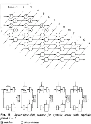
shown in Fig. 5, which uses the design shown in Fig. 2b.

One extra delay element is added to computational link

I , so that roll-back can be avoided. After delay transfer, the latency increases but data throughput rate does not change. In fact, this scheme is the best choice when data throughput rate is the most important factor to be con- cerned. If a = 1, whichever scheme is selected, the hardware overhead is 100% over original SA but performance will be unaffected.

I t i m e L l 2 3

Fig. 5 Space-time-shqt scheme for systolic array with pipelining period a = I

N matcher 0 delay element

3.2.2 IX = 2 case: For a transformation T which results the pipeline period a 2 2, the time schedule function W

has two alternatives. One can be described for k

.

W’

(scaled W ) and the other cannot be scaled. In the first case, all PES simultaneously activate for one clock cycle and idle for the next, alternately. In the latter case, PE,

activate alternate clock cycles exactly out of phase with their neighbours.

A space-shift scheme can only be used in the unscaled- W case. A space-shift FTSA is usually obtained by finding a suitable T n . For some algorithms, for example (Fig. 4a), only one PE overhead is needed and the resulting computing latency will not be different from that in the a = 1 case when this scheme is applied.

A time-shift scheme is like a conventional time- redundancy scheme if the original W is a scaled time schedule function. In the band matrix-vector multiplica- tion example, when W = [2, 21 = 2 . [l, 11, S = [l, 01 are selected and kl = 0, k2 = 1 are chosen, a time-shift FTSA is accomplished. Note that it does not need to roll back and recompute when an error occurs. In the unscaled W case, a time-shift FTSA can still be obtained. An example is shown in Fig. 4b. A drawback of this scheme is that a roll-back is necessary to correct faults and the error latency will increase. The latency is, however, smaller than the space-shift scheme in general cases.

I E E P R O C E E D I N G S , Vol. 137, P t . E , N o . 3, M A Y 1990

A space-time-shift scheme can be applied to both scaled and unscaled time schedule functions. An example for unscaled W is shown in Fig. 4c. This scheme needs only one PE and k2 time units overheads, but it can detect both transient and permanent faults.

3.2.3 a 3 3 case: Any systolic array with a 3 3 can be designed as an error-detectable FTSA with any of the three types of schemes. An error-masking FTSA which offers better fault-tolerance capability can also be obtained with only a small hardware or time overhead, which will be described later. The time and hardware overheads for different error detection schemes are summarised in Table 2.

Table 2 : T i m e and h a r d w a r e overheads f o r different error detection schemes

error detection time overhead hardware overhead

~~ _____

a = 1 space-shift 0 space-time-shift tot

(no delay transfer) space-time-shift t , (delay transfer) a = 2 space-shift 0 time-shift K2 space-time-shift t,, a

>

3 space-shift 0 time-shift K2 space-time-shift tst

N,,,

N d 0 Ntot N,,, N d 0 N A Ntot

-

1 . NtOt is the total number of processor elements.

2. N d is the number of PES along one direction.

3. td is the number of additional delay time units along the computa- tional direction d , after delay transfer.

4 . K Z = l k 2 1 .

5 . t S , = l k 2 + k l W . d , I .

3.3 Fault-tolerant systolic array design with concurrent error masking

In the error masking approach, which is known as N-tuple modular redundancy, N copies ( N odd) of a module and a majority voter are used to mask the error from failed module. At least three modules are necessary in a voting system which is typically called a triple modular redundancy (TMR). It seems that we need at least 200 percent hardware overhead for fault tolerance. In practice, it needs to put triplicate computations to the voter and then gets a correct result. The triplicate computations (ODG and 2 RDGs) may be computed in different PES and/or at different time. Using space-shift, time-shift or space-time-shift, we may obtain a better FTSA whose performance is acceptable. For example, an error masking systolic array which corresponds to a space-shift scheme with a = 2 systolic array has been proposed, and this hardware overhead is about 50 percent [SI. When space-shift scheme is used to a systolic array with a = 3 it needs only a very small amount of hardware overhead for a 1-dimensional array, i.e.

O(l/N,,,), where N,,, is total number of PES. Surely, the time overhead increases. But in some applications, time overhead may not be over 100 percent. The kind of array structures and redundancy schemes that are chosen depend on the user’s requirements for hardware and time cost. In the following, three redundancy schemes will be investigated to design FTSA with error masking for different a.

(7)

3.3.1 a = 1

case:

A space-shift scheme is like the conventional TMR scheme in which triplicated PES are tightly coupled.

A time-shift scheme cannot be used because each PE is active in any clock cycle.

A space-time-shift FTSA is obtained by shifting RSAl by k2, time units and RSA2 by k2, time units from OSA. If the results of OSA and RSAl are not correct before being used by next PES, the rollback problem occurs. This problem can be solved if delay transfer rule is applied such that at least K2 = Max

{

I

k2,I,

I

k2,

I

}

delay elements existing in computational link. No matter whatever scheme is selected, the hardware overhead is 200%.

3.3.2 cx = 2

case:

In this case, the utilisation of the PE is

half so that RSAl and OSA can merge into one SA and execute R D G l and O D G correctly. Another SA is necessary to execute RDG2.

A space-shift scheme shifts R D G l with respect to O D G and then transforms them into a FTSA, thereafter, an extra redundant PE is tightly coupled to FTSAs PE

whose sum of indexes is odd (or even). This result is similar to that in Reference 8 of which the hardware overhead is 50 percent only. Meanwhile, there may be no time overhead in some applications, for example, band matrix-vector multiplication.

There is no time-shift scheme because an extra systolic array is always necessary for a = 2 case.

The space-time-shift used as in subsection 3.2.2 and then adding extra SA, obrains a pseudo space-time-shift scheme. It is called pseudo because some replicated com- putations are executed simultaneously and some are executed at different time.

3.3.3 a = 3

case:

For a given non-full pipelining systolic

array with a = 3, for example, banded matrix-matrix multiplication [l], each PE activates one clock cycle and idles the next 2 clock cycles alternatively. Using these idle resources to execute two replicated computations pipelining can be filled, the efficiency of SA increased, and therefore the time and hardware overhead will become small.

In a space-shift scheme, a space-shift FTSA is obtained by suitably shifting R D G l and RDG2 to ODG. The band matrix multiplciations is taken as an example. Fig.

O23 a12 a22

a32

Fig. 6

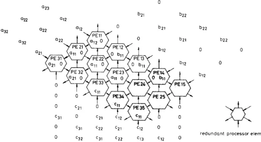
6 shows the systolic array with space-shift scheme while Fig. 7 show the operations in three consecutive cycles. In the original design [l], the gray PES are active and the other PES are idle in each cycle. In our design, one gray

PE and two redundant PES execute the same computations to perform a TMR scheme. In this example, it needs only 2N extra PES instead of 2N2 PES to perform TMR

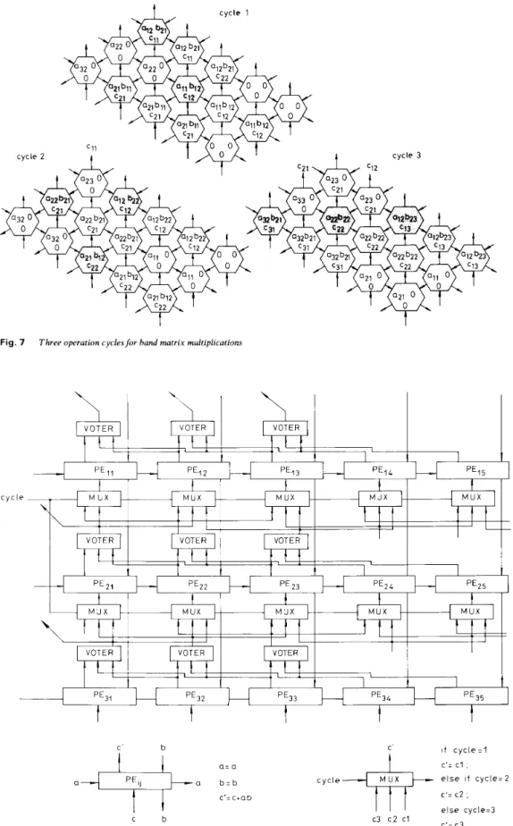
scheme. The detail architecture of this array is shown in Fig. 8. The voter takes the three results to vote and broadcast the result to three multiplexers. Note that each multiplexer takes the data from there different voters at three different cycles under the control signal, cycle, respectively.

The time-shift scheme is only applied in the case which has a computational link including Max

{

I

k2,I,

I

k2,

I

} or more delay elements. Otherwise, the erroneous result may be passed to next PE before being corrected.

This space-time-shift scheme can also be applied by selecting suitable transformation

T:,

.

As a summary, the time and hardware overheads for different error masking schemes are listed in Table 3.

Table 3: Time and hardware overheads for different error masking schemes

error masking time overhead hardware overhead

a = 1 space-shift 0 2NtOt

space-time-shift t,, 2Ntot

space-time-shift f d 2Nmt

(no delay transfer) (delay transfer) N t o t a = 2 space-shift 0 - + N t o t space-time-shift ts, N t o t Nd time-shift X X

2N,,,

a 2 3 space-shift 0 Nd time-shift K2 0 N t o t space-time-shift t,,

-

Nd 1. N,,, is the total number of processor elements. 2. N, is the number of PES along one direction.

3. t , is the number of additional delay time units along the compu- tational direction d, after delay transfer.

4. K2 = Max {lk2,1, lk2,I. lk2, -k2,I}.

5. t,, = Max { t , . I , , t12}, where tl = lk2, + k l . W . d, 1 , t z = lk2, + k l , . W . d , I a n d t l , = l k 2 , + & l , ~ W ~ d l - k 2 , - k l , W . d , I . 0 b 2 l b22 a 2 1 0 ‘31 c22 c21 ‘12 0 ‘32 c31 c 2 2 ‘13 c12

Systolic arrayfor band matrix multiplications with space-shft scheme

b 2 2 b 2 2

0 0

0

b12

redundant processor element

(8)

!

cycle 1

cycle 2 cycle 3

‘ T ‘

Fig. 7 Three operation cycles f o r band matrix multiplications

c y c l e -

‘ Y ‘

PE14

U+

1 I

VOTER VOTER I I

1 1

‘€31 PE34 PE35

I

t

C b C _{i f}_{c v c l e = l} c’= c l , e l s e i f c y c l e = 2 c‘= c2 , e l s e cycle=3

+ ’

C’=C3 a b - b c y c l e c ’ = c + a b c3 c 2 c l a = a c b

Fig. 8 Detailed architecture ofsystolic array f o r band matrix multiplications

(9)

4 Conclusions

A systematic design methodology for a redundant systolic array has been proposed. Redundancy schemes which consist of i) a space-shift, ii) a time-shift and iii) a space- time-shift schemes can be applied to fault tolerant systolic array design in order to detect (or mask) permanent fault, transient fault or both. By this design method, various redundancy designs for different utilisation efi- ciency, a, of PE in systolic array can result. According to the performance requirements including throughput rate, latency, block pipeline period, capability of fault detection (or masking) and hardware cost, a customised optimal redundant systolic array design can be achieved. 5 Acknowledgment

This work was supported by the National Science Council, Taiwan ROC, under grant NSC 77-0404-EO09- 04.

References

KUNG, H.T.: ‘Why systolic architectures?, Computer, 1982, 15, 1, pp. 3 7 4 6

FORTES, J.A.B., and RAGHAVENDRA, C.S. : ‘Gracefully Degrad- able Processor Arrays’, IEEE Trans., 1985, C-34, 11, pp. 1033-1044 KOREN, I.: ‘A Reconfigurable and Fault-Tolerant VLSI Multipro- cessor Array’. Proc. 8th Int. Symp. Computer Architecture, 1981, pp. 4 2 5 4 2

HUANG, K.H., and ABRAHAM, J.A. : ‘Algorithm-Based Fault Tol- erance for Matrix Operations’, IEEE Trans., 1984, C-33, 6, pp. 5 18-528 5 6 7 8 9 10 11 12 13 14 15 16

LIU, C.M., and JEN, C.W.: ‘On the Design of Algorithm-Based Fault-Tolerant VLSI Array Processor’, IEE Proc. E, 1989, 136, (6), SAMI, M.G., and STEFANELLI, R.: ‘Reconfigurable Architecture for VLSI Processing Array’. National Computer Conf., 1983, pp. ROSENBERG, A.L.: ‘The Diogenes Approach to Testable Fault- Tolerant Arrays of Processors’, IEEE Trans., 1983, C-32, 10, pp. 902-9 10

KIM, J.H., and REDDY, S.M.: ‘A Fault-Tolerant Systolic Array Using TMR method’. Proc. IEEE Internat. Conference Computer Design: VLSI in Computers, 1985, pp. 769-773

PATEL, J.H., and FUNG, L.Y.: ‘Concurrent Error Detection in ALUs by Recomputing with Shifted Operands’. IEEE Trans., 1982, JEN, C.W., KUNG, S.Y., and CHANG, C.W.: ‘Fault-Tolerant Design for VLSI Array Processors’. Proc. of Real-Time System Symp., 1987, pp. 4 6 6 4

CHAN, S.W., LEUNG, S.S., and WEY, C.L.: ‘Systematic Design Strategy for Concurrent Error Diagnosable Iterative Logic Arrays’,

Proc. IEE P t . E, 135, 2, 1988, pp. 87-94

CHAN, S.W., and WEY, C.L.: ‘The Design of Concurrent Error Diagnosable Systolic Arrays for Band Matrix Multiplications’. Proc. IEEE Trans. on CAD, 1988, pp. 21-37

KUNG, H.T., and LAM, M.S.: ‘Wafer-Scale Integration and Two- Level Pipelined Implementations of Systolic Arrays’, J . Parallel and Distributed Computing, 1984, pp. 32-63

KUNG, S.Y.: ‘VLSI Array Processors’, Prentice-Hall, 1988 NAVARRO, J.J., LLABERIA, J.M., and VALERO, M.: ‘Solving Matrix Problems with no Size Restriction on a Systolic Array Pro- cessor’. Proc. of Internat. Conf. on Parallel Processing, 1986, pp. 676683

NAVARRO, J.J., LLABERIA, J.M., and VALERO, M.: ‘Computing Size-Independent Matrix Problems on Systolic Array Processors’. Proc. 13th Internat. Symp. Computer Architecture, 1986, pp. 27 1-278

pp. 539-547

565-577

C-31,7, pp. 589-595