技術授權與平行交易課題之研究

全文

(1)國立高雄大學應用經濟學系碩士論文技術授權與平行交易課題之研究. Essays on Licensing and Parallel Trade. 研究生：梁育維撰指導教授：王鳳生博士. 中華民國一百零一年七月.

(2) 致謝詞第一次來到高雄生活及學習，彷彿昨日情景。在碩士生活快結束的同時，首先要感謝我的指導老師，王鳳生教授平日對我的諄諄教誨，總能在我論文上有瓶頸時適時給予我方向。還有辛苦的口試委員李仁耀老師與楊雅博老師給予我論文上寶貴的建議，使我的論文的修改更加完美。還要感謝我的同學們，佳志、俊儫、文宏、文婷、歆雅、浚濠及美麗的天使詩雅，無論生活上或課業上總能給我很大的鼓勵與激盪。還要感謝珮瑜與姿宇姐，這一年來貼心地協助我們處理論文零碎的流程及研討會相關的事情。還有感念學長姐及學弟妹，碩一時有學長姐的照顧；碩二時有學弟妹的噓寒問暖，我順利畢業了！最後當然最感謝我的父母，謝謝你們永遠的支持我走自己的路。讓我無後顧之憂的完成學業，未來的日子我會用任何方式讓你們幸福。感謝兩年來在我生活中出現的每個人、事、物，有你們真好。. 梁育維謹誌於國立高雄大學中華民國一百零一年夏. I.

(3) 技術授權與平行交易課題之研究. 指導教授：王鳳生博士國立高雄大學應用經濟系. 學生：梁育維國立高雄大學應用經濟系. 摘要. 第二章在三種授權方法下擁有專利權的公司會偏好選擇技術持股授權方法，來使其利潤極大。同時發現，若授權後選擇單位授權及固定費用授權利潤都為零。對消費者而言，若市場規模減去邊際成本過小時，不能確定何種方法較優；若介於某一範圍之間則單位授權方法優於固定費用授權,而固定費用授權優於技術持股授權方法; 若等於某一值時則技術持股授權與固定費用授權無異，但都比單位授權方法較差;若過大時, 則單位授權優於技術持股授權且同時技術持股授權優於固定收費授權方法。第三章延續第一篇架構增加研究及發展變數且內生求解後，主要證明擁有專利權的廠商其排序偏好則為選擇技術持股授權、固定費用授權與單位授權。而就被授權廠商來說，其排序偏好則為固定費用授權、單位授權與技術持股授權方法。以消費者及社會福利而言，單位授權方法會優於其他方法。第四章証明在最適關稅下，對於在兩國生產的廠商及在市場規模小且擁有較高 II.

(4) 生產力國的消費者而言，平行貿易是有利可圖的。但對市場規模大且低生產力國的消費者而言平行貿易有可能是無利可圖的。. 關鍵字：授權金、平行貿易、生產力差異 III.

(5) Essays on Licensing and Parallel Trade. Advisor: Dr. Leonard F.S. Wang Department of Applied Economics National University of Kaohsiung. Student: LIANG, YO-WEI Department of Applied Economics National University of Kaohsiung. ABSTRACT. Licensing is an increasing trend of industrial economy. Licensing usually uses two methods: per-unit royalty and fixed fee royalty. It hardly ever mentioned cross ownership. In this thesis, a duopoly model with ex-ante productivity difference is based for exploring the choice of endogenous R&D and licensing contract that includes per-unit royalty, fixed fee royalty and cross ownership. In addition, the parallel trade in a duopoly model with ex-ante productivity difference is used to analyze the welfare effect of parallel trade. In Chapter 2, we show that the licenser prefers cross ownership to other licensing methods. If the market size is too small, priority of licensing cannot be certain. If the market size is in a parametric range, consumers prefer per-unit royalty to fixed fee royalty and cross ownership; however, if the market size is too large, consumers prefer per-unit royalty to cross ownership and cross ownership is superior to fixed fee royalty.. IV.

(6) In Chapter 3, we show that the innovator still prefers cross ownership to fixed fee royalty and fixed fee royalty is superior to per-unit royalty. However, the licensee prefers fixed fee royalty to per-unit royalty and per-unit royalty is superior to cross ownership. Per-unit royalty method is the best from consumer surplus and social welfare perspectives. In chapter 4, we show that under optimal tariff, parallel trade is profitable and consumers are better-off in a country with a small market size and high productivity. However, consumers’ welfare is uncertain in a country with a large market size and low productivity.. Keywords: License royalty, Parallel trade, Productivity spread. V.

(7) CONTENTS CHAPTER ONE: Introduction ...................................................................................... 1 1.1 Motivation ........................................................................................................ 1 1.2 Research Background ...................................................................................... 1 1.3 Literature Review............................................................................................. 2 CHAPTER TWO: Licensing Contract and Consumer Welfare in Cournot Duopoly .... 4 2.1 Basic Setting .................................................................................................... 4 2.2 Benchmark: Pre-licensing ................................................................................ 5 2.3 Per-Unit Royalty .............................................................................................. 6 2.4 Cross Ownership .............................................................................................. 7 2.5 Fixed Fee Licensing ......................................................................................... 9 2.6 Summary ........................................................................................................ 13 CHAPTER THREE: Research and Development, Licensing and Social Welfare in Cournot Duopoly. ................................................................................................. 15 3.1 Basic Settings ................................................................................................. 15 3.2 Benchmark: Research and Development ....................................................... 16 3.3 Fixed Fee Royalty .......................................................................................... 17 3.4 Per-Unit Royalty ............................................................................................ 19 3.5 Cross Ownership Royalty .............................................................................. 22 3.6 Comparison of Licensing Royalty ................................................................. 23 3.7 Summary ........................................................................................................ 25 CHAPTER FOUR: Optimal Tax Policy and Parallel Trade ........................................ 26 4.1 Basic Settings ................................................................................................. 26 4.2 Benchmark: No Parallel Trade ....................................................................... 27 4.3 Parallel Trade Model ...................................................................................... 28 4.4 Summary ........................................................................................................ 32 CHAPTER FIVE: Conclusion ..................................................................................... 33. VI.

(8) CHAPTER ONE: Introduction 1.1 Motivation. In recent years, the industry made a large investment in Research and Development. When he got the technology patent, he can choose whether license to another one. Also, considering the royalty exist differential charge ways. But we can find many Taiwan’s companies still do Original Equipment Manufacturer (OEM) like Hon Hai Precision Industry Co. Type of manufacturers usually produced goods in Taiwan partially and produced goods in oversea partially. In Taiwan often see ECFA which was a quite special case, not just because Taiwan and Mainland China had quasi-enemy relationships. The population of China was larger than the population of Taiwan, and in general, Taiwan had higher technology while China had lower labor cost. I think who benefits from parallel trading with two countries. All consumers? All broker? All people live in Taiwan?. 1.2 Research Background. In chapters two and three, the welfare with licensing in duopoly markets received trermendous attention. There are three mainly developing direction of this literatures. One direction of literature shows that the patentee will prefer the fixed fee way to a per-unit royalty. The second direction of the literature shows that welfare may be higher under Cournot competition than under Bertrand competition. The third direction of the literature shows that in a duopolistic industry produces a homogeneous good, an internal patentee will always prefer licensing a non-drastic. 1.

(9) innovation by means of cross ownership royalty than by means of a per-unit royalty. And cross ownership royalty licensing hurts consumers because of the collusive effect that it induces. In chapter four, on the literature of parallel trade, Mukherjee and Zhao (2012) point out that parallel trade is profitable in a two-country trade model with unionization in one market. They show that the wage reducing effect of parallel trade in unionized markets may make parallel trading beneficial to a manufacturer.. 1.3 Literature Review. Martín and Saracho (2010) conclude from the empirical evidence that royalties, in particular ad valorem royalties, play an important role in licensing contracts. It is important to understand why licensing by means of ad valorem royalties may be preferred to other licensing ways The theoretical literature has focused on explaining the presence of royalties by considering per-unit royalties. Early work by Kamien and Tauman (1986) consider an external patentee and homogeneous good under Cournot oligopoly. They show that in the patentee will prefer the fixed fee to a per-unit royalty. Mukherjee (2010) considered licensing a new product in an economy with unionized labor market, and shows that the payoff of an outside innovator may be higher under royalty licensing than under fixed-fee licensing, if bargaining power of the labor union is sufficiently high. Mukherjee (2010) use a very simple but useful structure to show that under fixed-fee licensing, consumer surplus and welfare are higher under Cournot competition if the technological difference between the firms is moderate. Under royalty licensing, if the bargaining power of the licenser is not very. 2.

(10) high and the technological difference between the firms is large, consumer surplus and welfare are higher under Cournot competition. Mukherjee and Zhao (2012) provide a strategic reason for profitable parallel trading, by showing that parallel trade may be profitable to a manufacturer in the presence of labor unions, which creates imperfection in the factor market.. The logic. for our result is as follows. Parallel trade generally tends to reduce the profit of the manufacturer by increasing product market competition, even if it may augment the demand of the manufacturer. However, we find that it also tends to increase the profit of the manufacturer by reducing the unionized wage. This wage reducing effect (along with the demand augmenting effect) may dominate the competition intensifying effect to make parallel trading profitable to the manufacturer.. 3.

(11) CHAPTER TWO: Licensing Contract and Consumer Welfare in Cournot Duopoly Most of productivity licensing agreement observe empirically include either per-unit royalty. The theoretical literature generally focuses on per-unit royalty. We provide a simple justification for the presence of ad valorem and fixed fee royalties in licensing contract.. 2.1 Basic Setting. In this paper we assume that in the classic homogeneous good Cournot duopoly. Consider a country have two firms, with the inverse market demand function. P=a−Q. (2.1). With Q = ∑2i=1 q i , i =1,2。a, q ≥ 0, where q i represent totally quantity produces by firm i=1, 2. One of the firms which without loss of generality we will assume that firm 1 productivity is greater than firm 2. There is no transport cost. This paper has three sections in our analysis: (i) Per-unit royalty licensing (ii) Cross ownership royalty licensing (iii) Fixed fee royalty licensing. We will discuss licensing by three differences ways of license how the licensor’s profit changed in the three stages game. The analysis is modeled as a non-cooperative game in three stages. In the first stage, the productivity patentee chooses per-unit royalty, cross ownership and fixed fee royalty on a take-it-or-leave-it. In the second stage, firm 2 decides whether or not to accept the offer from firm 1. In lastly stage, both firms competition in a non-cooperative quantity competition game. See superscript F, a, p and NL represent respectively fixed fee, cross ownership, per-unit 4.

(12) royalties and no licensing below.. 2.2 Benchmark: Pre-licensing. First, we have to know no licensing situation on the two firms’ profit. The maximized the following object function to maximize its profit: Max π1NL = (p − c)q1. (2.2). Max πNL 2 = (p − λc)q 2 , λ > 1. (2.3). Where λ represent productivity spread. First-order conditions for profit maximization for each representative firm are as follows: ∂πNL 1 ∂q1 ∂πNL 2 ∂q2. = a − 2q1 − q 2 − c = 0 = a − q1 − 2q 2 − λc = 0. Solving these first-order conditions simultaneously, we can derive the equilibrium outputs in no licensing as follow: qNL 1 =. a+(λ−2)c. qNL 2 =. a+(1−2λ)c. (2.4). 3. (2.5). 3. Straightforward to show that a + (λ − 2)c and a + (1 − 2λ)c should be positive or zero. And checking second order condition is negative that provides the conditions profit will be maximizes. Using backward induction derive the optimal firms’ profit. ∗. 1. ∗. 1. π1NL = q∗1 2 = 9 [𝑎 + (𝜆 − 2)𝑐]2. (2.6). π𝑁𝐿 = 𝑞2∗ 2 = 9 [𝑎 + (1 − 2𝜆)𝑐]2 2. (2.7). 5.

(13) 2.3 Per-Unit Royalty. Second, we have to know per-unit royalty licensing situation on the two firms. Firm 1 licenses the technology to firm 2 and firm 1’ profit will be better after licensing. And firm 2 licensee’s cost of production will be equal to firm 1’s by licensing. MAX π1𝑝 = (𝑝 − 𝑐)𝑞1 + 𝑟𝑞2. (2.8). 𝑝. MAX π2 = (𝑝 − 𝑐)𝑞2 − 𝑟𝑞2. (2.9). Where r represent per-unit royalty. The intersection of these reaction functions gives the firms’ Cournot equilibrium quantities. Solving these first-order conditions simultaneously, we can derive the equilibrium outputs in per-unit royalty licensing as follow: ∂π1𝑝 = 𝑎 − 2𝑞1 − 𝑞2 − 𝑐 = 0 ∂q1 ∂π𝑝2 = 𝑎 − 𝑞1 − 2𝑞2 − 𝑐 − r = 0 ∂q 2 ∂2 π1𝑝 = −2 < 0 ∂q12 ∂2 π𝑝2 = −2 < 0 ∂q 2 2 Using Cramer’s rule can find the optimal output of downstream firms as follow: 𝑞1∗ =. 𝑎−(𝑐−𝑟). q∗2 =. 𝑎−(𝑐+2𝑟). (2.10). 3. (2.11). 3. Straightforward to show that 𝑎 − (𝑐 − 𝑟) and 𝑎 − (𝑐 + 2𝑟) should be positive or zero. And checking second order condition is negative that provides the conditions profit will be maximizes. Using backward induction we look for the optimal firms’ 6.

(14) profit: ∗. 1. 1. π1𝑝 = 𝑞12 + 𝑟𝑞2 = 9 [𝑎 − (𝑐 − 𝑟)]2 + 3 𝑟[𝑎 − (𝑐 + 2𝑟)] ∗. 1. π𝑝2 = 𝑞22 = 9 [𝑎 − (𝑐 + 2𝑟)]2. (2.12) (2.13). If r is greater than (𝜆 − 1)𝑐, firm 2 will not buy license. In first stage the productivity patentee will choose the per-unit royalty that maximizes his total revenues, that is the sum of the profits from his own production plus the licensing revenues, taken into account the restrictions given by the second and third stages of the game. In the optimal contract, 𝑟 = (𝜆 − 1)𝑐 must be true. If 𝑟 < (𝜆 − 1)𝑐 in the optimal contract, then one can increase the firm 1’s profit without violating the other constraints by adding to the r by a very small number. Let us first consider the situation where the licensing contract involves only an upfront per-unit. The upfront per-unit is given by 𝑟 = (𝜆 − 1)𝑐, we obtain: p. {. 1. Max π1. 1. s. t r ≤ (λ − 1)c, q1 = 3 [a − (c − r)], q 2 = 3 [a − (c + 2r)]. (2.14). As a result, the profit under the per-unit royalty will be equal to: 1. π1𝑝 = 𝑞12 + 𝑟𝑞2 = 9 {[𝑎 + 𝑐(−2 + 𝜆)]2 + 3𝑐(−1 + 𝜆)(𝑎 + 𝑐 − 2𝑐𝜆)} π𝑝2 = 𝑞22 = ( 𝐶𝑆 𝑝 =. 𝑄2 2. 𝑎−3𝑐 2 ) 3. (2.15) (2.16). 1. = 9 (2𝑎 − 𝑐(1 + 𝜆))2. (2.17). 2.4 Cross Ownership. Repeat again the games. At the third stage each firm look for an optimal output that maximizes his profits given valorem royalty (d) set the first stage. π1𝑎 = (𝑝 − 𝑐)𝑞1 + 𝑑(𝑝 − 𝑐)𝑞2. (2.18) 7.

(15) π𝑎2 = (1 − 𝑑)(𝑝 − 𝑐)𝑞2. (2.19). First-order conditions for profit maximization for each representative firm under cross ownership royalty licensing as follows: ∂π1𝑎 = a − 2q1 − q 2 − c − dq 2 = 0 ∂q1 ∂π𝑎2 = −(1 − 𝑑)𝑞2 + (1 − 𝑑)(a − q1 − q 2 − c) = 0 ∂q 2 Solving these first-order conditions simultaneously, we can derive the equilibrium outputs under cross ownership royalty licensing as follow: q∗1 =. (𝑎−𝑐)(1−𝑑). (2.20). 3−𝑑 𝑎−𝑐. q∗2 = 3−𝑑. (2.21). We can find the relationship between output of firm 1 and quantity of firm 2. q∗1 = (1 − 𝑑)q∗2. (2.22). The optimal profit of firm 1 by using the relationship between q∗1 and q∗2 . 𝒂−𝒄. ∗. π1𝑎 = (𝑎 − 𝑞1 − 𝑞2 − 𝑐)𝑞1 + 𝑑(𝑎 − 𝑞1 − 𝑞2 − 𝑐)𝑞2 = q∗2 2 = (𝟑−𝒅)𝟐. (2.23). In the optimal contract, 𝜋2𝑎 = 𝜋2𝑁𝐿 must be true. If 𝜋2𝑎 > 𝜋2𝑁𝐿 in the optimal contract, then one can increase the firm 1’s profit without violating the other constraints by adding to the d by a very small number. Let us first consider the situation where the licensing contract involves only an upfront cross ownership. The upfront cross ownership is given by π1𝑑 = π1𝐹 , we obtain: {. Max π1a. s. t q∗1 =. (a−c)(1−d) 3−d. , q∗2 =. a−c 3−d. , πa2 ≥ πNL 2. (2.24). 𝜋2𝑎 = 𝜋2𝑁𝐿 𝑎−𝑐 2 1 ) = [𝑎 + (1 − 2𝜆)𝑐]2 3−𝑑 9. (1 − 𝑑) ( 𝑑∗ =. 3(𝑎2 −4𝑎𝑐+𝑐 2 +2𝑎𝜆𝑐+2𝜆𝑐 2 −2𝜆2 𝑐 2 ). (2.25). 2(2𝑎2 −5𝑎𝑐+2𝑐 2 +𝑎𝜆𝑐+𝜆𝑐 2 −𝜆2 𝑐 2 ). 8.

(16) 𝜋1𝑎 =. 2. 4(𝑎+𝑐(−2+𝜆)) (−2𝑎+𝑐+𝜆𝑐)2. (2.26). 81(𝑎−𝑐)2. 𝐶𝑆 𝑎 =. (5𝑎2 −8ac−2aλc+𝑐 2 (5+2𝜆2 )−2λc2 ). (2.27). 9(a−c). 2.5 Fixed Fee Licensing. Finally, this model we discuss that firm 2 will buy license and pay a fixed fee to firm 1. π1𝐹 = (𝑝 − 𝑐)𝑞1 + 𝐹. (2.28). π𝐹2 = (𝑝 − 𝑐)𝑞2 − 𝐹. (2.29). Where F represents fixed fee. First-order conditions for profit maximization for each representative downstream firm are as follows: ∂π𝐹 1 ∂q1 ∂π𝐹 2 ∂q2. = 𝑎 − 2𝑞1 − 𝑞2 − 𝑐 = 0 = 𝑎 − 𝑞1 − 2𝑞2 − 𝑐 = 0. Solving these first-order conditions simultaneously, we can derive the equilibrium outputs under fixed fee licensing as follow: 1. q∗1 = 3 (a − c). (2.30). 1. q∗2 = 3 (a − c). (2.31). Straightforward to show that (a − c) should be positive or zero. And checking second order condition is negative that provides the conditions profit will be maximizes. Let us first consider the situation where the licensing contract involves only an upfront fixed fee. The upfront fee is given by π1𝑑 −π1𝐹 = 0, we obtain π1𝐹 = π1𝑁𝐿. 9.

(17) ⇒. (𝑎−𝑐)2 9. 1. + 𝐹 = 9 [𝑎 + (𝜆 − 2)𝑐]2. 1. ⇒ F = 9 [𝑎 + (𝜆 − 2)𝑐]2 −. (𝑎−𝑐)2 9. 1. = 9 [2𝑎 + (𝜆 − 3)𝑐](𝜆 − 1)𝑐. (2.32). Under fixed fee licensing, the profit of firm 1 and firm 2 is ∗. 𝑎−𝑐 2 ) 3. ∗. 𝑎−𝑐 2. π1𝐹 = 𝑞1∗ 2 + 𝐹 = (. π𝐹2 = 𝑞2∗ 2 − 𝐹 = (. 3. 1. + 9 [2𝑎 + (𝜆 − 3)𝑐](𝜆 − 1)𝑐 1. ) − 9 [2𝑎 + (𝜆 − 3)𝑐](𝜆 − 1)𝑐. 2. CS 𝐹 = 9 (𝑎 − 𝑐)2. (2.33) (2.34) (2.35). Table1、Comparison of Firm 1’s Profit under Different Licensing Contracts Profit of Patent-Holding Firm 1 1 π1NL = q∗1 2 = [𝑎 + (𝜆 − 2)𝑐]2 9. No Licensing. Per-Unit Royalty. Cross Ownership Royalty Fixed fee. π1𝑝 = 𝑞12 + 𝑟𝑞2 =. 1 {[𝑎 + 𝑐(−2 + 𝜆)]2 + 3𝑐(𝜆 − 1)(𝑎 + 𝑐 − 2𝜆𝑐)} 9 2. 𝜋1𝑎. 4(𝑎 + 𝑐(−2 + 𝜆)) (−2𝑎 + 𝑐 + 𝜆𝑐)2 = 81(𝑎 − 𝑐)2. 1 ∗ π1𝐹 = {(𝑎 − 𝑐)2 + [2𝑎 + (𝜆 − 3)𝑐](𝜆 − 1)𝑐} 9. By comparing the profits under a per-unit royalty and cross ownership we may establish the following proposition1: Proposition2.1.If the licensee willing to pay the royalty fee and the market scale be largest than marginal cost, in a duopolistic industry that produces a homogeneous good the licenser will always prefer cross ownership royalty to per unit royalty licensing when the licensing be happened. 10.

(18) Proof: 1. 𝑍0 = 𝜋1𝑃 − 𝜋1𝑎 = 9 {[𝑎 + 𝑐(−2 + 𝜆)]2 + 3𝑐(𝜆 − 1)(𝑎 + 𝑐 − 2𝜆𝑐)} − 𝟐. 𝟒(𝒂+𝒄(−𝟐+𝝀)) (−𝟐𝒂+𝒄+𝝀𝒄)𝟐 𝟖𝟏(𝒂−𝒄)𝟐 1. 𝑍0 =. 9(𝑎−𝑐)2 {[𝑎+𝑐(−2+𝜆)]2 +3𝑐(𝜆−1)[𝑎+𝑐−2𝜆𝑐]}−{[2[𝑎+𝑐(−2+𝜆)](−2+𝑐+𝜆𝑐)]4 }2 81(𝑎−𝑐)2. 𝐴 = 9(𝑎 − 𝑐)2 {[𝑎 + 𝑐(−2 + 𝜆)]2 + 3𝑐(𝜆 − 1)[𝑎 + 𝑐 − 2𝜆𝑐]} 1. 𝐵 = {[2[𝑎 + 𝑐(−2 + 𝜆)](−2 + 𝑐 + 𝜆𝑐)]4 }2 𝐴2 − 𝐵 2 = (𝐴 + 𝐵)(𝐴 − 𝐵) 4. = −16(𝑎 + 𝑐(−2 + 𝜆)) (−2𝑎 + 𝑐 + 𝜆𝑐)4 2. + 81(𝑎 − 𝑐)2 [(𝑎 + 𝑐(−2 + 𝜆)) + 3𝑐(−1 + 𝜆)(𝑎 + 𝑐 − 2𝜆𝑐)]. 2. When 𝜆 → 1, 𝐴2 − 𝐵 2 = 81(𝑎 − 𝑐)6 − 256(𝑎 − 𝑐)8 < 0 .We can find that 𝐵 > 𝐴 if A and B is positive.. By comparing the profits under a per-unit royalty and under fixed fee royalty, we may establish the following proposition2:. Proposition2.2. In a homogeneous duopolistic industry, the licenser’s profit is indifferent when it chooses per unit royalty licensing or fixed fee licensing if the productivity difference after licensing is vanished.. Proof: 𝑍1 = π1𝑝 − π1𝐹. 11.

(19) =. 1 {[𝑎 + 𝑐(−2 + 𝜆)]2 + 3𝑐(𝜆 − 1)(𝑎 + 𝑐 − 2𝜆𝑐)} 9 1 − {(a − c)2 + [2a + (λ − 3)c](λ − 1)c} 9 1. = 3 𝑐(𝜆 − 1)(𝑎 + 𝑐 − 2𝜆𝑐) When𝜆 → 1 ⇒ 𝑍1 → 0. By comparing the consumer surplus under a per-unit royalty, cross ownership and fixed fee royalty we may establish the following proposition 2.3:. Proposition2.3. After licensing contract is chosen, changes on consumer surplus determined by the parameter on market size minus the marginal cost.. Proof: The inequality holds 𝐶𝑆 𝑎 < 𝐶𝑆 𝐹 < 𝐶𝑆 𝑝 , 𝐶𝑆 𝑎 = 𝐶𝑆 𝐹 < 𝐶𝑆 𝑝 and 5. 5. 5. 𝐶𝑆 𝐹 < 𝐶𝑆 𝑎 < 𝐶𝑆 𝑝 respectively when4 < (𝑎 − 𝑐) < 2, (𝑎 − 𝑐) = 2 and 5. (𝑎 − 𝑐) > . 2 1. 4. 𝐶𝑆 𝑝 = 9 (2𝑎 − 𝑐(1 + 𝜆))2 when λ → 1,𝐶𝑆 𝑝 = 9 (𝑎 − 𝑐)2 𝐶𝑆 𝑎 =. (5𝑎2 −8ac−2aλc+𝑐 2 (5+2𝜆2 )−2λc2 ) 9(a−c) 2. CS 𝐹 = 9 (𝑎 − 𝑐)2 𝐶𝑆 𝑝 𝐶𝑆 𝑎. =. 4 (𝑎−𝑐)2 9 5(𝑎−𝑐) 9. =. 4(𝑎−𝑐) 5 5. 𝐶𝑆 𝑝 = 𝐶𝑆 𝑎 𝑤ℎ𝑒𝑛(𝑎 − 𝑐) = 4 5. 𝐶𝑆 𝑝 > 𝐶𝑆 𝑎 𝑤ℎ𝑒𝑛(𝑎 − 𝑐) > 4 5. 𝑝 𝑎 {𝐶𝑆 < 𝐶𝑆 𝑤ℎ𝑒𝑛(𝑎 − 𝑐) < 4. 12. when λ → 1, 𝐶𝑆 𝑎 =. 5(𝑎−𝑐) 9.

(20) 𝐶𝑆 𝑝 CS𝐹. 4. = 92 9. (𝑎−𝑐)2 (𝑎−𝑐)2. =2. 𝐶𝑆 𝑝 > 𝐶𝑆 𝐹 𝐶𝑆 𝑎 CS𝐹. =. 5(𝑎−𝑐) 9 2 (𝑎−𝑐)2 9. 5. = 2(𝑎−𝑐) 5. 𝐶𝑆 𝑎 = 𝐶𝑆 𝐹 𝑤ℎ𝑒𝑛(𝑎 − 𝑐) = 2 5. 𝐶𝑆 𝑎 > 𝐶𝑆 𝐹 𝑤ℎ𝑒𝑛(𝑎 − 𝑐) > 2 5. 𝑎 𝐹 {𝐶𝑆 < 𝐶𝑆 𝑤ℎ𝑒𝑛(𝑎 − 𝑐) < 2. 2.6 Summary. This paper prepared to do a simple justification for why we may observe cross ownership rather than per-unit royalties or fixed fee royalties in productivity technology licensing contracts. Martín and Saracho (2010) show that ad valorem royalty rather than per-unit royalties in patent licensing contracts. In a Cournot duopoly model when one of the firm licenses to his rival a cost reducing innovation, this type of royalty allows the patentee to strategically commit to be less aggressive. This effect, in turn, implies that consumer surplus is lower with licensing than without it. Our analysis relies on the assumption that the patentee is firm 1. Our result we have shown that (i) cross ownership licensing can be superior to fixed-fee licensing and per-unit licensing for the patent-holding firm. (ii) If licenser will license for the productivity technology and the licensee accept it, we can find have four situations of consumer surplus of three license way. First, when the market scale minus marginal. 13.

(21) 5. cost is very small (𝑎 − 𝑐) ≤ 4, any situations of consumer surplus of the license way is uncertain；Second, when the market scale minus marginal cost is. 5 4. 5. < (𝑎 − 𝑐) < 2. for consumer, per-unit royalty prefer to fixed fee royalty and fixed fee prefer to cross 5. ownership；Third, when the market scale minus marginal cost is (𝑎 − 𝑐) = 2 for consumer, per-unit royalty prefer to fixed fee royalty and cross ownership, indifference between fixed fee royalty and cross ownership；Forth, when the market scale minus marginal cost is (𝑎 − 𝑐) >. 5 2. for consumer, per-unit royalty prefer to. cross ownership royalty and cross ownership royalty prefer to fixed fee.. 14.

(22) CHAPTER THREE: Research and Development, Licensing and Social Welfare in Cournot Duopoly. Mukherjee (2010) is the main inspiration of our works. They used a very simple but useful structure to capture under fixed fee royalty licensing, consumer surplus and welfare are higher under Cournot competition if the technological difference between the firms is moderate. Under royalty licensing, if the bargaining power of the licenser is not very high and the technological difference between the firms is large, consumer surplus and welfare are higher under Cournot competition. We add to cross ownership way with Research and Development in Duopoly market. To understand which licensing ways is better when endogenous solving R&D.. 3.1 Basic Settings. Consider a country have two firms, with the inverse market demand function P=1−Q. (3.1). Where Q represent totally quantity produced by firm i=1,2 . One of the firms which without loss of generality we will assume is firm 1 own goods produced cost is greater than firm 2. Because firm 1 investments capital to do the research and development and makes his cost reducing. There is no transport cost. This paper has three sections in our analysis: (i) Per-unit royalty licensing , (ii) Cross ownership royalty licensing, (iii) Fixed-fee royalty licensing. We will discuss licensing by three differences ways how the licensor’s profit changed in the four. 15.

(23) stages game. The analysis is modeled as a non-cooperative game in four stages. In the first stage, the firm 1 determined the research and development value. In the second stage, the firm owns cost advantages by research and development sets a per-unit royalty, cross ownership royalty and fixed fee royalty on a take-it-or-leave-it. In the third stage, firm 2 decided whether or not to accept the offer from firm 1. In lastly stage, both firms competition in a non-cooperative quantity competition game. See superscript F, a, p and R&D represent respectively fixed fee, cross ownership, per-unit royalties and Research& Development below.. 3.2 Benchmark: Research and Development. First, we have to know only firm 1 engage research and development. The maximized the following object function to maximize its profit: 1. 𝜋1 = [𝑃 − (𝑐 − 𝑥)]𝑞1 − 𝑥 2. (3.2). 2. 𝜋2 = [𝑃 − 𝑐]𝑞2 Where x represent the firm 1 engage the research and development value. First-order conditions for profit maximization for each representative firm are as follows: 𝜕𝜋1 = 1 − 2𝑞1 − 𝑞2 − 𝑐 + 𝑥 = 0 𝜕𝑞1 𝜕𝜋2 = 1 − 𝑞1 − 2𝑞2 − 𝑐 = 0 𝜕𝑞2 𝜕 2 𝜋1 = −2 < 0 𝜕𝑞1 2 𝜕 2 𝜋2 = −2 < 0 𝜕𝑞2 2 Solving these first-order conditions simultaneously, we can derive the equilibrium outputs in firm 1 engage the research and development as follow: 16. (3.3).

(24) 𝑞1∗ =. 1+2𝑥−𝑐. 𝑞2∗ =. 1−𝑥−𝑐. (3.4). 3. (3.5). 3. Straightforward to show that (1 + 2𝑥 − 𝑐) and (1 − 𝑥 − 𝑐) should be positive or zero. And checking second order condition is negative that provides the conditions profit will be maximizes. Using backward induction derive the optimal firms’ profit. We use quantity in substitution for the profits function and consumer surplus as follow: 1. 1. 1. 𝜋1𝑅&𝐷 = (𝑞1∗ )2 − 2 𝑥 2 = 9 (1 + 2𝑥 − 𝑐)2 − 2 𝑥 2 1. 𝜋2𝑅&𝐷 = (𝑞2∗ )2 = 9 (1 − 𝑐 − 𝑥)2. (3.6) (3.7). First-order conditions for profit maximization for firm 1 are as follows: 𝑥 ∗ = (1 − 𝑐)2. (3.8) 1. 1. 𝜋1 𝑅&𝐷 |𝑥=𝑥 ∗ = 9 (1 + 2𝑥 ∗ − 𝑐)2 − 2 𝑥 ∗ 2 = (1 − 𝑐)2 𝜋2 𝑅&𝐷 |𝑥=𝑥 ∗ = 𝑐 2 (3 − 𝑐)2 𝐶𝑆 𝑅&𝐷 =. 𝑄2. 𝑆𝑊 𝑅&𝐷 =. 2. 9. (3.10). 2. = 9 (1 − c)2. 11. (3.9). (3.11). (−1 + 𝑐)2 + (−3 + 𝑐)2 𝑐 2. (3.12). 3.3 Fixed Fee Royalty. Second, we have to know fixed fee royalty licensing situation on the two firms. Firm 1 licenses the technology of cost reducing by R&D to firm 2 and firm 1’ profit will be better after licensing. We discuss that firm 2 will buy license and pay a fixed fee to firm 1. The maximized the following object function to maximize its profit: 17.

(25) 1. 𝜋1𝐹 = [𝑃 − (𝑐 − 𝑥)]𝑞1 − 𝑥 2 + 𝐹. (3.13). 2. 𝜋2𝐹 = [𝑃 − (𝑐 − 𝑥)]𝑞2 − 𝐹 (3.14) Where F represents fixed fee. First-order conditions for profit maximization for each representative firm are as follows: 𝜕𝜋1 = 1 − 2𝑞1 − 𝑞2 − 𝑐 + 𝑥 = 0 𝜕𝑞1 𝜕𝜋2 = 1 − 𝑞1 − 2𝑞2 − 𝑐 + 𝑥 = 0 𝜕𝑞2 𝜕 2 𝜋1 = −2 < 0 𝜕𝑞1 2 𝜕 2 𝜋2 = −2 < 0 𝜕𝑞2 2 Solving these first-order conditions simultaneously, we can derive the equilibrium outputs under fixed fee licensing as follow: 1. 𝑞1∗ = 3 (1 + 𝑥 − 𝑐). (3.15). 1. 𝑞2∗ = 3 (1 + 𝑥 − 𝑐). (3.16). Straightforward to show that (1 + 𝑥 − 𝑐) should be positive or zero. And checking second order condition is negative that provides the conditions profit will be maximizes. 1. 1. 1. 𝜋1𝐹 = 𝑞1∗ 2 − 2 𝑥 2 + 𝐹 = 9 (1 + 𝑥 − 𝑐)2 − 2 𝑥 2 + 𝐹. (3.17). 𝜋2𝐹 = 𝑞2∗ 2 − 𝐹 (3.18) 𝑅&𝐷 𝑅&𝐷 𝐹 𝐹 In the optimal contract, 𝜋2 = 𝜋2 must be true. If 𝜋2 > 𝜋2 in the optimal contract, then one can increase the firm 1’s profit without violating the other constraints by adding to the F by a very small number. Let us first consider the situation where the licensing contract involves only an upfront fixed fee. The upfront fixed fee is given by π1𝑑 = π1𝐹 , we obtain {. 1. Max π1F. s. t q∗1 = q∗2 = 3 (1 + x − c), πF2 ≥ πR&𝐷 2 18. (3.19).

(26) 𝜋2𝐹 = 𝜋2𝑅&𝐷 ⟹. 1 1 (1 + 𝑥 − 𝑐)2 − 𝐹 = (1 − 𝑐 − 𝑥)2 9 9 4. ⟹ 𝐹 ∗ = 9 (1 − 𝑐)𝑥 ∗. 𝜋1𝐹 =. (1+𝑥−𝑐)2 9. 1. (3.20) 4. − 2 𝑥 2 + 9 (1 − 𝑐)𝑥. (3.21). First-order conditions for profit maximization for firm 1 are as follows: ∗. 𝜕𝜋1𝐹 2 4 = (1 + 𝑥 − 𝑐) − 𝑥 + (1 − 𝑐) = 0 𝜕𝑥 9 9 ∗. 𝜕 2 𝜋1𝐹 −7 = <0 2 𝜕𝑥 9 After checking second order condition is negative that provides the conditions profit will be maximizes. We can find the optimal R&D value. Using backward induction derive the optimal R&D value. We use R&D value in substitution for the profits function of firm 1 and consumer surplus as follow: ∗. 6. 𝑥 𝐹 = 7 (1 − 𝑐) ∗. 25. ∗. 1. (3.22). 𝜋1𝐹 |𝑥=𝑥 ∗ = 63 (1 − 𝑐)2. (3.23) 2. 4. 155. 𝜋2𝐹 |𝑥=𝑥 ∗ = [3 (1 + 𝑥 − 𝑐)] − 9 (1 − 𝑐)𝑥 = 147 (1 − 𝑐)2 CS 𝐹 =. 𝑄2. 𝑆𝑊 𝐹 =. 2. = 2(1 − 𝑐)2. 1522 441. (3.24) (3.25). (1 − 𝑐)2. (3.26). 3.4 Per-Unit Royalty. We have to know per-unit royalty licensing situation on the two firms. Firm 1 licenses the technology by R&D to firm 2 and after licensing firm 1’ profit will be better than in non-licenses. And firm 2 licensee’s cost of middle production will be. 19.

(27) equal to firm 1’s. We discuss that firm 2 will buy license and pay a per-unit royalty to firm 1. The maximized the following object function to maximize its profit: 1. 𝜋1𝑝 = [𝑃 − (𝑐 − 𝑥)]𝑞1 − 2 𝑥 2 + 𝑟𝑞2. (3.28). 𝜋2𝑝 = [𝑃 − (𝑐 − 𝑥)]𝑞2 − 𝑟𝑞2 (3.29) Where r represents per-unit royalty. First-order conditions for profit maximization for each representative firm are as follows: 𝜕𝜋1 𝑝 = 1 − 2𝑞1 − 𝑞2 − 𝑐 + 𝑥 = 0 𝜕𝑞1 𝜕𝜋2 𝑝 = 1 − 𝑞1 − 2𝑞2 − 𝑐 + 𝑥 − 𝑟 = 0 𝜕𝑞2 𝜕 2 𝜋1 𝑝 = −2 < 0 𝜕𝑞1 2 𝜕 2 𝜋2 𝑝 = −2 < 0 𝜕𝑞2 2 The intersection of these reaction functions gives the firms’ Cournot equilibrium quantities. Solving these first-order conditions simultaneously, we can derive the equilibrium outputs in per-unit royalty licensing as follow: 1. 𝑞1∗ = 3 (1 + 𝑥 − 𝑐 − 𝑟). (3.30). 1. 𝑞2∗ = 3 (1 + 𝑥 − 𝑐 − 2𝑟). (3.31). Straightforward to show that(1 + 𝑥 − 𝑐 − 𝑟) and (1 + 𝑥 − 𝑐 − 2𝑟) should be positive or zero. And checking second order condition is negative that provides the conditions profit will be maximizes. In the optimal contract, 𝑟 = 𝑥 must be true. If 𝑥 > 𝑟 in the optimal contract, then one can increase the firm 1’s profit without violating the other constraints by adding to the r by a very small number. Let us first consider the situation where the licensing contract involves only an. 20.

(28) upfront per-unit royalty. The upfront per-unit royalty fee is given by 𝑟 = 𝑥, we obtain 1. p. Max π1 = [P − (c − x)]q 2 − 2 x 2 + rq 2. { 1 1 s. t r ≤ x, q∗1 = 3 (1 + x − c − r), q∗2 = 3 (1 + x − c − 2r). (3.32). 1 𝜋 𝑝 1 |𝑟=𝑥 = (𝑞1∗ )2 − 𝑥 2 + 𝑟𝑞2∗ 2 =. 1 1 𝑟 (1 + 𝑥 − 𝑐 − 𝑟)2 − 𝑥 2 + (1 + 𝑥 − 𝑐 − 2𝑟) 9 2 3 1. 1. 𝑥. = 9 (1 − 𝑐)2 − 2 𝑥 2 + 3 (1 − 𝑐 − 𝑥). (3.33). First-order conditions for profit maximization for firm 1 are as follows: 𝜕𝜋1 1 = −𝑥 + (1 − 𝑐 − 2𝑥) = 0 𝜕𝑥 3 𝜕 2 𝜋1 5 = − <0 𝜕𝑥 2 3 After checking second order condition is negative that provides the conditions profit will be maximizes. We can find the optimal R&D value. Using backward induction derives the optimal R&D value. We use the optimal R&D value in substitution for the profits function of firm 1 and consumer surplus as follow: 1. 𝑥 𝑝 ∗ = 3 (1 − 𝑐) 𝜋 𝑝 1 |𝑥=𝑥 ∗ =. (3.34). 1 1 𝑥∗ (1 − 𝑐)2 − (𝑥 ∗ )2 + (1 − 𝑐 − 𝑥 ∗ ) 9 2 3. 7. = 54 (1 − 𝑐)2. (3.35). 4. 𝜋 𝑝 2 |𝑥=𝑥 ∗ = 81 (1 − 𝑐)2 CS 𝑝 =. 𝑄2 2. (3.36). 25. = 162 (1 − 𝑐)2. (3.37). 1. 𝑆𝑊 𝑝 = 3 (1 − 𝑐)2. (3.38). 21.

(29) 3.5 Cross Ownership Royalty. Repeat the games. At the fourth stage each firm look for an optimal output that maximizes his profits given cross ownership royalty (d) and R&D value (x) in both firms accept the contract. 1. 𝜋1𝑎 = [𝑃 − (𝑐 − 𝑥)]𝑞1 − 2 𝑥 2 + 𝑑(𝑃 − (𝑐 − 𝑥))𝑞2 𝜋2𝑎 = (1 − 𝑑)[𝑃 − (𝑐 − 𝑥)]𝑞2 Where d represents cross ownership royalty. First-order conditions for profit. (3.39) (3.40). maximization for each representative firm are as follows: ∂𝜋1𝑎 = 1 − 2𝑞1 − 𝑞2 − 𝑐 + 𝑥 − 𝑑𝑞2 = 0 ∂𝑞1 ∂𝜋2𝑎 = (1 − 𝑑)(1 − 𝑞1 − 2𝑞2 − 𝑐 + 𝑥) = 0 ∂𝑞2 ∂2 𝜋1𝑎 = −2 < 0 ∂𝑞1 2 ∂2 𝜋2𝑎 = −2(1 − 𝑑) < 0 ∂𝑞2 2 The intersection of these reaction functions gives the firms’ Cournot equilibrium quantities. We can derive the equilibrium outputs in cross ownership royalty licensing as follow: 𝑞1 =. (1−𝑑)(1+𝑥−𝑐). 𝑞2 =. (1+𝑥−𝑐). (3.41). (3−𝑑). (3.42). (3−𝑑). Straightforward to show that (1 − 𝑑)(1 + 𝑥 − 𝑐) and (1 + 𝑥 − 𝑐) should be positive or zero. Checking second order condition is negative that provides the conditions profit will be maximizes and finally, we can derive a relationship with equilibrium output of firm 1 and firm 2.. 22.

(30) 1 Max π1 = [1 − q1 − q 2 − (c − x)]q1 − x 2 + d[1 − q1 − q 2 − (c − x)]q 2 2 (1 − d)(1 + x − c) (1 + x − c) s. t q1 = , q2 = , πa2 ≥ πR&𝐷 2 (3 − d) (3 − d) { (3.43) In the optimal contract, 𝑟 = 𝑥 must be true. If 𝑥 > 𝑟 in the optimal contract, then one can increase the firm1’s profit without violating the other constraints by adding to the r by a very small number. Let us first consider the situation where the licensing contract involves only an upfront cross ownership royalty. The upfront cross ownership royalty fee is given by 𝜋2𝑎 = 𝜋2𝑅&𝐷 we obtain: 𝜋2𝑎 = 𝜋2𝑅&𝐷 18(1−𝑐+𝑥). d∗ = 3 + −8+𝑐 2 +(−11+𝑥)𝑥+𝑐(7+2𝑥). (3.44). 𝜋1∗ |𝑑=d∗ 1. = 324 ((−8 + 7𝑐 + 𝑐 2 )2 + 2(−1 + 𝑐)(8 + 𝑐)(−11 + 2𝑐)𝑥 + 3(−19 + 2(−5 + 𝑐)𝑐)𝑥 2 + 2(−11 + 2𝑐)𝑥 3 + 𝑥 4 ) First-order conditions for profit maximization for firm 1 are as follows:. (3.45). ∂𝜋1∗ 1 (−1 + 𝑐 + 𝑥)(−88 + 2𝑐 2 + 𝑥(−31 + 2𝑥) + 𝑐(5 + 4𝑥)) = 0 = ∂x 162 ∂2 𝜋1∗ <0 ∂x 2 𝑥 𝑎 ∗ = (1 − 𝑐). (3.46). 1. ∗. 𝜋1𝑎 |𝑥=x∗ = 2 (1 − 𝑐)2. (3.47). ∗. 𝜋2𝑎 |𝑥=x∗ = 0. (3.48). 1. CS 𝑎 = 2 (1 − 𝑐)2. (3.49). 𝑆𝑊 𝑎 = (1 − 𝑐)2. (3.50). 3.6 Comparison of Licensing Royalty. 23.

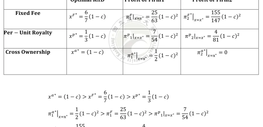
(31) Considering licensing strategy under optimal R&D, we obtain the following proposition.. Proposition 3.1.The optimal cross ownership royalty is larger than the optimal fix fee royalty and the fixed fee royalty is larger than the optimal per-unit royalty. ∗. 1. 25. 7. Proof: 𝜋1𝑎 |𝑥=x∗ = 2 (1 − 𝑐)2 > 𝜋1𝐹 = 63 (1 − 𝑐)2 > 𝜋 𝑝 1 |𝑥=𝑥 ∗ = 54 (1 − 𝑐)2 .. Table 2: Comparison of Profits and Optimal R&D under Different Licensing Contracts 𝐎𝐩𝐭𝐢𝐦𝐚𝐥 𝐑&𝐃. 𝐏𝐫𝐨𝐟𝐢𝐭 𝐨𝐟 𝐅𝐢𝐫𝐦𝟏. 6 (1 − 𝑐) 7. 𝜋1𝐹 |𝑥=𝑥 ∗ =. 𝐏𝐞𝐫 − 𝐔𝐧𝐢𝐭 𝐑𝐨𝐲𝐚𝐥𝐭𝐲. 1 𝑥 𝑝 ∗ = (1 − 𝑐) 3. 𝜋 𝑝 1 |𝑥=𝑥 ∗ =. 𝐂𝐫𝐨𝐬𝐬 𝐎𝐰𝐧𝐞𝐫𝐬𝐡𝐢𝐩. 𝑥 𝑎 ∗ = (1 − 𝑐). 𝐅𝐢𝐱𝐞𝐝 𝐅𝐞𝐞. ∗. 𝑥𝐹 =. ∗. 𝑥 𝑎 ∗ = (1 − 𝑐) > 𝑥 𝐹 = ∗. 𝜋1𝑎 |𝑥=x∗ = ∗. 𝜋2𝐹 |𝑥=𝑥 ∗ =. 𝐏𝐫𝐨𝐟𝐢𝐭 𝐨𝐟 𝐅𝐢𝐫𝐦𝟐. 155 25 ∗ (1 − 𝑐)2 (1 − 𝑐)2 𝜋2𝐹 | ∗ = 𝑥=𝑥 147 63 7 (1 − 𝑐)2 54. 1 ∗ 𝜋1𝑎 |𝑥=x∗ = (1 − 𝑐)2 2. 𝜋 𝑝 2 |𝑥=𝑥 ∗ =. 4 (1 − 𝑐)2 81. ∗. 𝜋2𝑎 |𝑥=x∗ = 0. 6 1 (1 − 𝑐) > 𝑥 𝑝 ∗ = (1 − 𝑐) 7 3. 1 25 7 (1 − 𝑐)2 > 𝜋 𝑝 1 |𝑥=𝑥 ∗ = (1 − 𝑐)2 (1 − 𝑐)2 > 𝜋1𝐹 = 2 63 54 155 4 (1 − 𝑐)2 > 𝜋 𝑝 2 |𝑥=𝑥 ∗ = (1 − 𝑐)2 > 𝜋2𝑎 ∗ | ∗ = 0 𝑥=x 147 81. Proposition3.2. Cross ownership royalty licensing hurts consumers because the licenser wrests the licensee’s profit of all, imply the licensee’s optimal output is decreasing after cross ownership license.. 24.

(32) Proof: 𝑆𝑊 𝐹 > 𝑆𝑊 𝑎 > 𝑆𝑊 𝑝 and CS 𝐹 > CS 𝑎 > CS 𝑝 Table3: Comparison of Consumer Surplus and Social Welfare under Different Licensing Contracts 𝐂𝐨𝐧𝐬𝐮𝐦𝐞𝐫 𝐒𝐮𝐫𝐩𝐥𝐮𝐬 𝐅𝐢𝐱𝐞𝐝 𝐅𝐞𝐞 𝐏𝐞𝐫 − 𝐔𝐧𝐢𝐭 𝐑𝐨𝐲𝐚𝐥𝐭𝐲 𝐂𝐫𝐨𝐬𝐬 𝐎𝐰𝐧𝐞𝐫𝐬𝐡𝐢𝐩. CS 𝐹 = 2(1 − 𝑐)2. CS 𝑝 =. 25 (1 − 𝑐)2 162. 1 CS 𝑎 = (1 − 𝑐)2 2. 𝐒𝐨𝐜𝐢𝐚𝐥 𝐖𝐞𝐥𝐟𝐚𝐫𝐞 𝑆𝑊 𝐹 =. 1522 (1 − 𝑐)2 441. 𝑆𝑊 𝑝 =. 1 (1 − 𝑐)2 3. 𝑆𝑊 𝑎 = (1 − 𝑐)2. 1 25 (1 − 𝑐)2 CS 𝐹 = 2(1 − 𝑐)2 > CS 𝑎 = (1 − 𝑐)2 > CS 𝑝 = 2 162 𝑆𝑊 𝐹 =. 1522 1 (1 − 𝑐)2 > 𝑆𝑊 𝑎 = (1 − 𝑐)2 > 𝑆𝑊 𝑝 = (1 − 𝑐)2 441 3. 3.7 Summary. Our analysis relies on the assumption that in a Cournot duopoly model when one of the firms licenses to his rival a cost reducing. Firm 1’s cost reducing by research and development. We show that licenser preferred cross ownership royalty to per-unit and fixed fee royalty in Chapter2, which echoes with the finding of Martín and Saracho (2010). Per-unit royalty method is the best from consumer surplus. And per-unit royalty method also is the best from social welfare. According to an aspect, we can show the licenser wrests the licensee’s all of profit, imply the licensee’s optimal output is decreasing after cross ownership license.. 25.

(33) CHAPTER FOUR: Optimal Tax Policy and Parallel Trade Here in Taiwan, we can hear about the discussion on parallel trade and partial oversea production and partial local production often. We change Mukherjee and Zhao’s model a little and make it able to illustrate this story. Like Taiwan had higher technology while China had lower labor cost. We analyze this problem below: the firm in the smaller scale country produced partially goods in home country and produced partially goods in foreign country. And, have a broker will purchase the goods produced by the firm of lager scale country’s like Mainland China. At the same time I studying a paper that Profitable parallel trade in unionized markets by Mukherjee and Zhao. Previous literature has generally believed that parallel trade reduces the profits of the manufacturers. We show that consumer surplus and social welfare changed if home country’s Government setting an optimal tariff tax and difference productivity between the two countries. The remainder of the paper is organized as follows. Section 2 discusses the model and derives the result. Section 3 concludes.. 4.1 Basic Settings. Consider a manufacturer, called M, which sells product in two countries, A and B. M has plant in each of Country A (the home country) and Country B (the foreign country). We assume the labor in Country A have great productivity than Country B. The𝜆 represents productivity differential factor (𝜆 > 1). There is not transportation cost for simplicity. And the inverse market demand in Country A is 𝑃𝑎 = 1 − 𝑞𝑎. 26.

(34) while it is Country B is 𝑃𝑏 = 𝑎 − 𝑞𝑏 , with a > 1 . Imply the market size in Country B is heavier than Country A. Given the manufacturer in two countries productivity cost is c. This structure is similar to the “Profitable parallel trade in unionized markets” case of Mukherjee and Zhao, which excludes union. We analyze the following moves of the game. At first stage, decision the optimal quantity. At second stage, export country’s Government attended to the social welfare and concluded the optimal tariff. The game is solved by backward induction.. 4.2 Benchmark: No Parallel Trade. First, we have to know no parallel trade situation on the firms’ profit of the two countries. The maximized the following object function to maximize its profit: 𝑀𝑎𝑥 𝑛𝑝 𝜋 = (𝑃𝑎 − 𝜆𝑐)𝑞𝑎 + (𝑃𝑏 − 𝑐)𝑞𝑏 𝑞𝑎 , 𝑞𝑏. (4.1). First-order conditions for profit maximization are as follows: 𝜕𝜋 𝑛𝑝 𝜕𝑞𝑎 𝜕𝜋 𝑛𝑝 𝜕𝑞𝑏. = 1 − 2𝑞𝑎 − 𝜆𝑐 = 0 = 𝑎 − 2𝑞𝑎 − 𝑐 = 0. 𝜕 2 𝜋 𝑛𝑝 = −2 < 0 𝜕𝑞𝑎 2 𝜕 2 𝜋 𝑛𝑝 = −2 < 0 𝜕𝑞𝑏 2 The equilibrium outputs in countries A and B are respectively. 1. 𝑞𝑎𝑛𝑝 = 2 (1 − 𝜆𝑐) ≥ 0. (4.2). 1. 𝑞𝑏𝑛𝑝 = 2 (𝑎 − 𝑐) ≥ 0. (4.3). Straightforward to show that (1 − 𝜆𝑐) and (𝑎 − 𝑐) should be positive or zero. And checking second order condition is negative that provides the conditions profit 27.

(35) will be maximizes. We can find the optimal quantities 𝑞𝑎𝑛𝑝 and 𝑞𝑏𝑛𝑝 and using backward induction derive the optimal profit, consumer surplus of two countries and social welfare in Country A. 2. 2. 1. 𝜋 𝑛𝑝 = (𝑞𝑎𝑛𝑝 ) + (𝑞𝑏𝑛𝑝 ) = 4 [(1 − 𝜆𝑐)2 + (𝑎 − 𝑐)2 ] 1. 2. 1. 1. 2. 1. 𝐶𝑆𝐴𝑛𝑝 = 2 (𝑞𝑎𝑛𝑝 ) = 8 (1 − 𝜆𝑐)2. (4.5). 𝐶𝑆𝐵𝑛𝑝 = 2 (𝑞𝑏𝑛𝑝 ) = 8 (𝑎 − 𝑐)2 𝑛𝑝. 𝑆𝑊𝐴. 𝑛𝑝. (4.4). (4.6). 1. = 𝜋 𝑛𝑝 + 𝐶𝑆𝐴 = 8 [3(1 − 𝜆𝑐)2 + 2(𝑎 − 𝑐)2 ]. (4.7). 4.3 Parallel Trade Model. Assume that there is a firm in Country B, called K, who buys the product of M in Country B and sells it to Country A. It is assumed that M the parallel trader derives utility only from profit but not from consumption. Firm K and the consumers of Country B demand for the product of M under parallel trade. Hence, under the parallel trade, output is 𝑞𝑏 − 𝑞𝑘 in Country B (𝑄𝐵 = 𝑞𝑏 − 𝑞𝑘 ) and output is 𝑞𝑎 + 𝑞𝑘 in Country A (𝑄𝐴 = 𝑞𝑎 + 𝑞𝑘 ). And the inverse market demand in country A is 𝑃𝑎 = 1 − 𝑄𝐴 while it is country B is 𝑃𝑏 = 𝑎 − 𝑄𝐵 with 𝑎 > 1.. We analyze the following game under parallel trade. At stage 1, M makes its production decisions, 𝑞𝑎 and 𝑞𝑏 and K choose 𝑞𝑘 , simultaneously, while K pays 𝑃𝐵 to purchase the product of M. At stage 2, the Government of Country A will decide the optimal tariff tax. The game is solved by backward induction. Given the K. 28.

(36) firm export the production no transportation cost. Firm M totally profit: Ｍ𝑎𝑥 𝜋 𝑝 = (𝑃 − 𝜆𝑐)𝑞 + (𝑃 − 𝑐)𝑞 𝑎 𝑎 𝑏 𝑏 𝑞𝑎 , 𝑞𝑏 First-order condition for profit maximization are as follows:. (4.8). 𝜕𝜋 𝑝 = 1 − 2𝑞𝑎 − 𝑞𝑘 − 𝜆𝑐 = 0 𝜕𝑞𝑎 𝜕𝜋 𝑝 𝜕𝑞𝑏. = 𝑎 − 2𝑞𝑏 − 𝑞𝑘 − 𝑐 = 0. 𝜕 2𝜋𝑝 = −2 < 0 𝜕𝑞𝑎 2 𝜕 2𝜋𝑝 = −2 < 0 𝜕𝑞𝑏 2 The intersection of these reaction functions gives the firms’ Cournot equilibrium quantities. Solving these first-order conditions simultaneously, we can derive the equilibrium outputs in parallel trade as follow: 1. 𝑞𝑎∗ = 2 (1 − 𝑞𝑘 − 𝜆𝑐) ≥ 0. (4.9). 1. 𝑞𝑏∗ = 2 (𝑎 − 𝑞𝑘 − 𝑐) ≥ 0 Straightforward to show that. (4.10) 1 2. (1 − 𝑞𝑘 − 𝜆𝑐) ≥ 0 and. 1 2. (𝑎 − 𝑞𝑘 − 𝑐) ≥ 0. should be positive or zero. And checking second order condition is negative that ensure the conditions profit will be maximizes. 𝑞𝑎∗ and 𝑞𝑏∗ substitution into the firm M’s profit and consumer surplus of the two countries. 1. 𝜋 𝑝 = (𝑞𝑎∗ )2 + (𝑞𝑏∗ )2 = 4 [(1 − 𝑞𝑘 − 𝜆𝑐)2 + (𝑎 − 𝑞𝑘 − 𝑐)2 ] 1. 1 1. 1. 1 1. 2. 𝐶𝑆𝐴𝑃 = 2 (𝑞𝑎 + 𝑞𝑘 )2 = 2 [2 (1 − 𝑞𝑘 − 𝜆𝑐) + 𝑞𝑘 ] ≥ 0 2. 𝐶𝑆𝐵𝑃 = 2 (𝑞𝑏 − 𝑞𝑘 )2 = 2 [2 (𝑎 − 𝑞𝑘 − 𝑐) − 𝑞𝑘 ] ≥ 0. (4.11) (4.12) (4.13). Firm K maximize the following expressions to determine their outputs: Max π = (Pa − Pb − t)qk = (1 − q a − q k − a + q b − q k − t)q k qk m 𝑞𝑎∗ and 𝑞𝑏∗ substitute into the firm K’s profit. 29. (4.14).

(37) 𝜋𝑚 = (1 − 𝑞𝑎 − 𝑞𝑘 − 𝑎 + 𝑞𝑏 − 𝑞𝑘 − 𝑡)𝑞𝑘 1. 1. = (1 − 2 (1 − 𝑞𝑘 − 𝜆𝑐) − 𝑞𝑘 − 𝑎 + 2 (𝑎 − 𝑞𝑘 − 𝑐) − 𝑞𝑘 − 𝑡) 𝑞𝑘. (4.15). First-order condition for profit maximization is as follows: 𝜕𝜋𝑚 1 = (1 − 𝑎 − 𝑐 − 2𝑡 + λc − 8𝑞𝑘 ) = 0 𝜕𝑞𝑘 2 𝜕 2 𝜋𝑚 = −4 < 0 𝜕𝑞𝑘 2 1. 𝑞𝑘 = 8 (1 − 𝑎 − 𝑐 − 2𝑡 + λc) ≥ 0. (4.16). Straightforward to show that (1 − 𝑎 + 𝜆𝑐 − 𝑐 − 2𝑡) ≥ 0 should be positive or zero. And checking second order condition is negative that provides the conditions profit will be maximizes. 𝑞𝑘∗ substitute for the firm K’s profit and the social welfare. Government of Country A maximizes the following expressions to determine his tariff tax. 2. 1. πm = (q∗k )2 = (8 (1 − 𝑎 − 𝑐 − 2𝑡 + λc) 𝑀𝑎𝑥 𝑡. (4.17). 𝑆𝑊𝐴𝑝 = 𝜋 𝑃 + 𝐶𝑆𝐴𝑝 + 𝑡𝑎𝑟𝑖𝑓𝑓. 1. 1. = 256 [(7 + 𝑎 + 𝑐 + 2𝑡 − 9𝜆𝑐)2 + (1 + 7𝑎 − 9𝑐 − 2𝑡 + 𝜆𝑐)2 ] + 512 (−9 + 𝑎 + 𝑡. 𝑐 + 2𝑡 + 7𝜆𝑐)2 + 4 (1 − 𝑎 + 𝜆𝑐 − 𝑐 − 2𝑡). (4.18). First-order condition for the social welfare maximization is as follows: 𝜕𝑆𝑊𝐴𝑝 =0 𝜕𝑡 𝜕 2 𝑆𝑊𝐴𝑃 <0 𝜕𝑡 2 Solving these first-order conditions, we can derive the equilibrium outputs as follows: 1. 𝑡 ∗ = 118 (35 − 43𝑎 − 11𝑐 + 19𝜆𝑐). (4.19). 1. The optimal policy is 𝜆 ≥ 19𝑐 (43𝑎 + 11𝑐 − 35). 𝜋𝑃 =. 4(28+𝑎+3𝑐−32𝜆𝑐)2 +(3−61𝑎+53𝑐+5𝜆𝑐)2 13924. 30. ≥0. (4.20).

(38) 𝑝. 𝐶𝑆𝐴 =. (−35+𝑎+3𝑐+27𝜆𝑐)2 6962. Tariff =. ≥0. (4.21). (−35+43𝑎+11𝑐−19𝜆𝑐)(−3+2𝑎+6𝑐−5𝜆𝑐) 6962. ≥0. (4.22). Proposition4.1. The equilibrium profit of M is higher under parallel trade than under no parallel trade. After parallel trade, consumer surplus of country A is better than no parallel trade. But we should be look at the cost whether approach to market scale of country A.. Proof: It’s straightforward to show that (56 + 61𝑎 − 53𝑐 − 64λc)(−3 + 2𝑎 + 6𝑐 − 5λc) 6962 1 𝑝 𝑛𝑝 We find that 𝜋 > 𝜋 if 1 ≤ 𝜆 ≤ 5𝑐 (−3 + 2𝑎 + 6𝑐) 𝜋 𝑝 − 𝜋 𝑛𝑝 =. The reason for the above result is as follows. 1 1 2 𝐶𝑆𝐴𝑝 − 𝐶𝑆𝐴𝑛𝑝 = [(𝑞𝑎 + 𝑞𝑘 )2 − (𝑞𝑎𝑛𝑝 ) ] = [𝑞𝑎 + 𝑞𝑘 + 𝑞𝑎𝑛𝑝 ][(𝑞𝑎 + 𝑞𝑘 ) − 𝑞𝑎𝑛𝑝 ] 2 2 𝑛𝑝 Let A = 𝑞𝑎 + 𝑞𝑘 and 𝐵 = 𝑞𝑎 . 1. 𝐴 − 𝐵 = (𝑞𝑎 + 𝑞𝑘 ) − 𝑞𝑎𝑛𝑝 = 59 (3 − 2𝑎 − 6𝑐 + 5𝜆𝑐). 1. If 𝜆 ≥ 5𝑐 (2𝑎 + 6𝑐 − 3), A − B would be positive, we can find 𝐶𝑆𝐴𝑝 > 𝐶𝑆𝐴𝑛𝑝 .. Proposition4.2. Consumer of low productivity of bigger market scale is too bad after parallel trade when firm M exist productivity spread. If the productivity spread infinitesimal consumer of country B is better after parallel trade. λ, Critical level of productivity difference which is larger, small or equal. The magnitude of 𝜆∗ huge on the market scale and production cost. 31.

(39) Proof: 2. 1. 1. 𝐶𝑆𝐵𝑝 − 𝐶𝑆𝐵𝑛𝑝 = 2 [(𝑞𝑏 − 𝑞𝑘 )2 − (𝑞𝑏𝑛𝑝 ) ] = 2 [𝑞𝑏 − 𝑞𝑘 + 𝑞𝑏𝑛𝑝 ][𝑞𝑏 − 𝑞𝑘 − 𝑞𝑏𝑛𝑝 ] Let A = 𝑞𝑏 − 𝑞𝑘 and 𝐵 = 𝑞𝑏𝑛𝑝 1. (𝑞𝑏 − 𝑞𝑘 ) − 𝑞𝑏𝑛𝑝 = (−3 + 2𝑎 + 6𝑐 − 5𝜆𝑐) 118 1 118 1 118 1. 1. (−3 + 2𝑎 + 6𝑐 − 5𝜆𝑐) > 0 ⇒ 𝜆 < 5𝑐 (−3 + 2𝑎 + 6𝑐) ⇒ 𝐶𝑆𝐵𝑝 > 𝐶𝑆𝐵𝑛𝑝 (−3 + 2𝑎 + 6𝑐 − 5𝜆𝑐) = 0 ⇒ 𝜆 =. 1. 5𝑐 1. {118 (−3 + 2𝑎 + 6𝑐 − 5𝜆𝑐) < 0 ⇒ 𝜆 > 5𝑐. (−3 + 2𝑎 + 6𝑐) ⇒ 𝐶𝑆𝐵𝑝 = 𝐶𝑆𝐵𝑛𝑝 (−3 + 2𝑎 + 6𝑐) ⇒ 𝐶𝑆𝐵𝑝 < 𝐶𝑆𝐵𝑛𝑝. 4.4 Summary. In this paper, we examined the strategic behavior of the country A’s Government decision the optimal tariff tax rate. If the country A’s Government determined the tariff tax approach the optimal tax, export country’s consumer whether better after parallel trade and finding whether an import country’s consumer is better after parallel trade? We can find the export country’s consumer surplus is reducing (increasing) if the productivity spread is approach to bigger (lower) and import country’s consumer surplus will be increase when. 1. 𝜆 ≥ 5𝑐 (2𝑎 + 6𝑐 − 3) after parallel trade.. 32.

(40) CHAPTER FIVE: Conclusion In chapter 2, in a duopolistic industry that produces a homogeneous good, if the market scale is not too small and r<. 𝑎−𝑐 2. , an internal licenser will always prefer per. unit royalty licensing to fixed fee licensing. But we know that within the range. 5 4. 5. 5. < (𝑎 − 𝑐) < 2 or (𝑎 − 𝑐) = 2 or. 5. (𝑎 − 𝑐) > , the licenser choose per-unit royalty which is better than cross ownership 2 and fixed fee royalty for consumer. Finally, excluding per-unit licensing, we show that when the difference between market scale and marginal cost is. 5 4. 5. < (𝑎 − 𝑐) < , the 2. licenser choose fixed fee royalty which is better than cross ownership royalty for 5. consumer. If (𝑎 − 𝑐) = 2, the licenser choose that fixed fee or cross ownership 5. royalty is indifference for consumer. If (𝑎 − 𝑐) > 2, the licenser choose cross ownership royalty which is better than fixed fee royalty for consumer. In chapter 3, we find the licenser still prefers cross ownership to fixed fee royalty and fixed fee royalty is superior to per-unit royalty. However, the licensee prefers fixed fee royalty to per-unit royalty and per-unit royalty is superior to cross ownership. Per-unit royalty method is the best from consumer surplus and social welfare. In chapter 4, we find that the export country’s consumer surplus is reducing. (increasing) if the productivity spread got larger (lower) and import country’s 1. consumer surplus will increase when 𝜆 ≥ 5𝑐 (2𝑎 + 6𝑐 − 3) after parallel trade.. 33.

(41) References Kabiraj, T. and Lee, C.C. (2011). ‘Technology Transfer in a Duopoly with Horizontal and Vertical Product Differentiation’, Trade and Development Review, 4, 19-40 Kamien, M.I. and Tauman, Y. (1986). ‘Fees versus Royalties and the Private Value of a Patent’, Quarterly Journal of Economics, 101, 471-491. Martín, M. S. and Saracho, A. I. (2010). ‘Royalty Licensing’, Economics Letters, 107, 284–287. Mukherjee, A. (2010). ‘Competition and Welfare: The Implications of Licensing’, The Manchester School, 78, 20-40. Mukherjee, A. (2010). "Licensing a New Product: Fee vs. Royalty Licensing with Unionized Labor Market’, Labour Economics, 17, 735-742. Mukherjee, A. and Zhao, L. (2012). ‘Profitable Parallel Trade in Unionized Markets’, Journal of Economics. Forthcoming. Wang, X. H. (1998). ‘Fee versus Royalty Licensing in a Cournot Duopoly Model’, Economics Letters, 60, 55-62.. 34.

(42)