Effects of Adsorbed Polymers on the Axisymmetric Motion of Two Colloidal Spheres

(1)

ARTICLE NO.CS975144

Effects of Adsorbed Polymers on the Axisymmetric Motion

of Two Colloidal Spheres

Jimmy Kuo and Huan J. Keh1

Department of Chemical Engineering, National Taiwan University, Taipei 106-17, Taiwan, Republic of China Received May 7, 1997; accepted August 19, 1997

advantages in relative insensitivity to the presence of electro-The effects of adsorbed polymer on the slow motion of two _{lytes, equal efficiency in both aqueous and nonaqueous} dis-spherical particles along the line of their centers are examined

persion, reversibility of flocculation, and equal efficiency at semianalytically. The particles may have unequal radii, and their

both high and low particle concentrations ( 1, 2 ) . Nowadays surface polymer layers are allowed to differ in characteristics. The

stabilization by either natural or synthetic polymers is ex-surface polymer layer on each particle is assumed to be thin

rela-ploited in a diverse range of industrial products ( e.g., paints, tive to the radius of the particle and to the surface-to-surface

glues, inks, lubricants, detergents, pharmaceutical and food distance between the particles. A method of matched asymptotic

emulsions ) and operative in many biological systems ( such expansions in small parameters li ( where i Å 1 and 2 ) combined

as blood and milk ) . with a boundary collocation technique is used to find the solution

for the creeping flow field within and outside the adsorbed polymer A polymer can adsorb on the surface of a colloidal particle layers, where li is the ratio of the polymer-layer length scale to as a result of van der Waals forces, hydrogen bonding,

Cou-the radius of particle i . The results for Cou-the hydrodynamic forces _{lombic ( charge – charge ) attraction, or dipole interactions. A} exerted on the particles in a resistance problem and for the particle _{balance must be struck in the affinity among the polymer,} velocities in a mobility problem are expressed in terms of the

the particle surface, and the solvent. The usual result is that effective hydrodynamic thicknesses ( Li) of the polymer layers,

the polymer is tied to the surface at a number of points but which are accurate to O ( l2

i) . The O ( li) term for Li normalized

for some of its length it is able to extend into the solution. by its value in the absence of the other particle is found to be

Sequences of segments lying on the surface form ‘‘trains,’’ independent of the polymer segment distribution, the

hydrody-which are separated by ‘‘loops,’’ while the ends of the poly-namic interactions among the segments, and the volume fraction

mer usually protrude into the solution as ‘‘tails’’ ( 3 – 6 ) . of the segments. The O ( l2

i) term for Li, however, is a sensitive

There is no unique measure of the thickness of a surface function of the polymer segment distribution and the volume

frac-tion of the segments. In general, the effects of particle interacfrac-tions polymer layer due to the diffuseness of the polymer chains. on the motion of polymer-coated particles can be quite significant, _{A convenient definition is the hydrodynamic thickness which} especially when the particles are moving in the opposite directions. _{reflects the additional viscous drag exerted by the polymer}

q 1997 Academic Press _{segments on the solvent motion relative to the particle. This}

Key Words: motion of two particles; adsorbed polymers; hydro- _{experimentally defined length is the thickness of a totally} dynamic thickness; particle interactions.

impermeable layer that would be required on the particle surface to produce the extra viscous drag. Several methods are available for determining the hydrodynamic thickness of INTRODUCTION

adsorbed polymer layers on colloidal particles, including photon correlation spectroscopy ( also known as quasielastic The increasing amount of work on the adsorption of

mac-light scattering or dynamic mac-light scattering ) ( 7 – 10 ) , micro-romolecules from solution onto solid surfaces is

understand-electrophoresis ( 11, 12 ) , sedimentation ( 13, 14 ) , and vis-able, considering the fundamental and practical interest of

cometry ( 15, 16 ) . It was found both theoretically ( 17 ) and the subject. One of the most spectacular effects of such

experimentally ( 9 ) that the hydrodynamic thickness of ad-adsorption is the ability of some polymers to stabilize

colloi-sorbed polymer layers is usually much larger than the layer dal dispersions with respect to aggregation of particles.

Com-thickness determined by ellipsometry ( 18, 19 ) and by neu-pared with an electrostatically stabilized dispersion,

adsorp-tron scattering ( 20 ) . tion of nonionic polymers to particle surfaces has prominent

The steady-state motion of a single spherical particle cov-ered by a layer of adsorbed polymers was analyzed by An-1

(2)

expansions to solve the Stokes flow equations within and outside the polymer layer. The result for the drag force ex-erted by the fluid on the translating particle, expressed as the hydrodynamic thickness of the adsorbed polymer layer, is accurate to O ( l2

) where l is the ratio of the polymer-layer characteristic thickness to the particle radius. Their calculations showed that ( i ) the O ( l2

) term is negative, meaning the hydrodynamic thickness increases as the parti-cle radius increases assuming all other conditions are con-stant, ( ii ) a free-draining model for flow through the polymer chains is a very good approximation for calculating the hy-drodynamic thickness if the Stokes radius of the polymer

FIG. 1. Geometrical sketch of two polymer-coated spheres moving segments is much smaller than the characteristic thickness

alone their line of centers. of the polymer layer, and ( iii ) the presence of only a small

amount of adsorbed polymer tails can make a significant contribution to the hydrodynamic thickness if the length

the line of their centers in an unbounded Newtonian liquid, scale of the tails exceeds the length scale of the loops by a

as shown in Fig. 1. Here, ( ri, ui, f ) are the spherical

coordi-factor of two or more. Recently, through the method of

nates measured from the center of particle i , where i equals matched asymptotic expansions, the quasisteady motion of

1 or 2. The origin of the cylindrical polar coordinate system a spherical particle coated with a layer of adsorbed polymers

( v_V , f, z ) is taken at the center of particle 1 for convenience. in a concentric spherical cavity has also been examined ( 22 ) .

The two particles, separated by a center-to-center distance In practical applications, many colloidal phenomena

in-d , may have arbitrary rain-dii, R1 and R2, and their surface

volve collaborative motion of several particles. If particles

polymer layers are allowed to differ in characteristics. The are randomly dispersed within a fluid, the most important

thickness of the surface polymer layer surrounding particle hydrodynamic interactions are those between a pair of

parti-i parti-is characterparti-ized by a length scale di ( based on loops if

cles. Using a method of reflections, Anderson and

Soloment-both loops and tails are present ) . In general, the length scale sev ( 23 ) analytically solved the mobility problem of two

of a surface polymer layer depends on the molecular weight arbitrarily oriented, identical spheres accounting for the

pres-of the polymer, the amount pres-of the polymer adsorbed, and ence of the surface layers on the particles. The mobility

the relative interactions among the polymer, interface, and coefficients accurate to O ( l2

) were determined in a power

fluid. It is assumed that di ! Ri and d1/ d2! d0( R1 / series of j up to O ( j5

) , where j is the ratio of particle

R2) , so these two thin surface layers will not overlap with radius to distance between the particle centers.

each other. The velocity of particle i equals Uiez, where ez

For the motion of two particles with a large separation, the

is the unit vector in the z direction. The Reynolds numbers power-series results from one or two reflections describe the

are assumed to be much smaller than unity. particle interactions adequately. However, when the particles

The fluid velocity and dynamic pressure fields, v and p , are close together, higher order interactions become significant

are governed by the modified Stokes equations ( 21 ) , and the leading terms in the asymptotic solution result in a

poor description of the particle-interaction effect. In the present

Ç r{ m[Ç_v_/₍Ç_{v )}T

] }0 Çp0z rf [ v0v( p )

]Å0 , [1a ] work, our objective is to obtain an exact solution to the

quasi-steady problem of two polymer-coated spheres moving along _{Ç r}_v_Å_0. _{[1b ]} the line of their centers to O(l2

). The particles may have

unequal radii and their surface polymer layers may have differ- _{In Eq. [1a ] , z is the friction coefficient of an isolated} poly-ent characteristics. The mompoly-entum equation applicable to the _{mer segment, r is the density of the polymer segments at} system is solved by using the method of matched asymptotic _{the position in question, v}( p )

is the velocity of the segments, expansions incorporated with a boundary collocation technique _{f is a function of r accounting for hydrodynamic interactions} (24). Our numerical results for the particle interactions

com-among segments, and m is the local fluid viscosity which is pare favorably with the formulas generated analytically from

also a function of r. The density distribution of the segments the method of reflections. It is found that the hydrodynamic

in the loops and tails cannot yet be determined experimen-interactions between polymer-coated particles can be

signifi-tally. Theoretical studies ( 5, 6 ) have established that the cant when the particles are almost in contact.

density of polymer segments in the loops decays exponen-ANALYSIS _{tially with the distance from the surface of adsorption and} the segment density in the tails can exceed the value in the Consider the quasisteady motion of two spherical

(3)

free-draining model for flow through the segments fÅ1, while The drag force ( in the z direction ) exerted by the fluid on the particle surface ri ÅRi is ( 25 )

segment – segment interactions cause f to increase with r. The effective viscosity m in the polymer layer is not a mea-surable quantity. Previous calculations for an isolated sphere

Fi Åpms

*

p 0 r3 isin3ui Ì Ìri

S

E2 C r2 isin2ui

D

ridui. [ 7 ]

( 21 ) have shown that the effects of the difference between m and the constant bulk solvent viscosity msare negligible.

Therefore, we assume mÅmsthroughout the surface polymer _{In terms of the equivalent hydrodynamic thickness L}

iof the

layers in this work. It is understood that v( p ) _Å

Uiezin the _{adsorbed polymer layer on particle i , the drag force can be}

surface layer surrounding the translating particle i . _{expressed by the Stokes law with a correction of the} two-Owing to the axisymmetric nature of the flow, it is conve- _{sphere hydrodynamic interaction,}

nient to introduce the Stokes stream function C which

satis-fies Eq. [1b ] and is related to the velocity components in _F

i Å 06pms( Ri /Li) UiKi. [ 8 ]

the spherical coordinate system ( r , u, f ) by

For the system specified by Eq. [ 6 ] , the correction factor for the interaction between two ‘‘bare’’ spheres Ki Å 02 Di 20/

£_rÅ 0 1

r2 sin u

ÌC

Ìu , [ 2a ] 3 RiUi, where Di 20 is defined by Eq. [13 ] . The

hydrody-namic thickness Li can be expressed as

£uÅ 1 r sin u ÌC Ìr . [ 2b ] Li ÅAiRili( 1 /Bili) /O ( l3i) . [ 9 ]

Taking the curl of Eq. [1a ] and applying Eqs. [1b ] and [ 2 ] _{By combining Eqs. [ 7 ] – [ 9 ] after solving Eqs. [ 3 ] and [ 6 ]} gives a fourth-order linear partial differential equation _{for C, one can obtain dimensionless parameters A}

i and Bi.

for C, _{Note that A}

iis positive and Bireflects the influence of

curva-ture of the surface of particle i . Also, Ai and Bi ( or Li) are

functions of the segment density distributions of the surface

E4 C0l02 i

S

biE 2 C/dbi dr ÌC

Ìr

D

Å0. [ 3 ] polymer layers and the parameters U2/ U1, R2/ R1, and ( R1

/ R2) / d . If the surface layer surrounding particle i is an impermeable dense film of thickness di, one has Ai Å1 and

Here i can be either 1 or 2, and the dimensionless parameters

Bi Å0. bi and li are defined as

Equation [ 3 ] poses a singular perturbation problem when li ! 1. In the ‘‘outer region,’’ in which ri 0 Ri @ Rili, bi Å

d2

iz rf ms

, [ 4a ] one has bi Å 0, and a sufficiently general solution for the

stream function is li Å di Ri , [ 4b ] C( O )_Å

∑

2 iÅ1

∑

` nÅ2 ( Cinr 0 n/ 1 i /Dinr 0 n/ 3 i ) G 01 / 2 n ( ni) , [10 ]

and the axisymmetric Stokesian operator E2

is given by _C

inÅCin0/Cin1li/Cin2l

2

i/ rrr, [11a ]

DinÅDin0/Din1li/Din2l

2 i/ rrr, [11b ] E2_Å Ì 2 Ìr2/ sin u r2 Ì Ìu

S

1 sin u Ì Ìu

D

. [ 5 ] where G01 / 2

n ( ni) is the Gegenbauer polynomial of the first

kind of order n and of degree 01

2 and ni is used to denote

In Eqs. [ 3 ] and [ 5 ] , dimensionless variables are used, with

cos ui for brevity. The Gegenbauer polynomials are related

r normalized by the particle radius Ri and C by UiR

2

i. The

to the Legendre polynomials via the relation parameter bidenotes the ratio of the frictional force exerted

by the polymer segments on the fluid to the viscous force

of the bulk fluid, and is O ( 1 ) with respect to li which has G01 / 2n ( n )Å

1

2n01[ Pn02( n )0Pn( n ) ] . [12 ] been assumed to be small. Equation [ 3 ] must be solved

subject to the boundary conditions

A solution in the form of Eq. [10 ] immediately satisfies boundary condition [ 6b ] . The unknown constants Cinmand

ri ÅRi; vÅUiez ( i Å1, 2 ) , [ 6a ]

Dinmin Eq. [11] are to be determined by matching C( O )with

the solution to Eq. [ 3 ] in the ‘‘inner regions.’’ The solution ( v_V2

/z2

)1 / 2_{r `}

(4)

of Cin0and Din0has been obtained numerically by Gluckman the constants Cinmand Dinmare to be determined by matching

Eqs. [10 ] and [15 ] at equivalent orders in li,

et al. ( 24 ) who studied the axisymmetric motion of two

‘‘bare’’ spherical particles using the boundary collocation

method. _lim yir` C( I ) i Ålim yir` [ C( O )_/1 2Uir2i( 1 0n2i) ]riÅRi/liyi. [18 ]

Substituting Eq. [10 ] into Eq. [ 7 ] and utilizing the orthog-onality properties of the Gegenbauer polynomials, we obtain

The second term in the brackets accounts for the difference the simple relation

in the reference frames used for C( O )

Fj n2 Rj / bj n 2 Rj y2 j 0bj ngjyj

DG

. [ 20b ] Ri d3 Fin3 dy3 i 0bi Ri dFin3 dyi Åcin, [17a ]

On the other hand, taking the differentiation of Eqs. [19c,

yi Å0: Fin3 Å

dFin3

dyi

Å0, [17b ]

d ] with respect to yitwice and solving them by utilizing the

orthogonality properties of the Gegenbauer polynomials, we obtain

where iÅ 1 or 2, n Å2, 3, 4, . . . , and cinare integration

constants to be determined by matching the inner and outer

solutions. _lim yjr` d2 Fj n2 dy2 j Å 0bj n, [ 21a ]

(5)

to define the variables Gj and Hj in Eq. [ 22 ] , the same lim yjr` d2 Fj n3 dy2 j Åcj n yj Rj

/dj n, [ 21b ] _{equations as Eqs. [ 23 ] – [ 26 ] will be obtained.}

The parameters Ai and Bi in Eq. [ 9 ] are obtained from

Eqs. [14 ] , [ 20 ] , [ 22 ] , and [ 26 ] as for jÅ1 or 2. In Eqs. [ 20 ] and [ 21] , gjis defined by Eq.

[ 28a ] , and the dimensionless constants sijn, pijn, qijn, bj n, cj n,

∑

` nÅ2 pijndj n/Vj

∑

` nÅ2 qijnbj n] , [ 27b ]

If we define new variables

GjÅ 1 bj2 dFj22 dyj , [ 22a ] _where HjÅ 1 cj2 dFj23 dyj , [ 22b ] _g_j_Å_lim y_jr` 1 Rj ( Gj/yj) , [ 28a ]

then Eqs. [16 ] , [17 ] , and [ 21] give _L_*_j _Å_lim

yjr` 1 Rj

S

H*j 0 y2 j 2 Rj

D

, [ 28b ] Rj d2 Gj dy2 j 0bj Rj GjÅ0, [ 23a ] _L jÅlim yjr` 1 Rj ( Gj 0yj) , [ 28c ] yjÅ0: GjÅ0, [ 23b ] VjÅ 1 R2 j

*

` 0 ( Gj/yj0Rjgj) dyj. [ 28d ] yjr `: dGj dyj r 01; [ 23c ]

In Eq. [ 27 ] , the numerical solution of Di 20 is known ( 24 )

and the constants sijn, pijn, qijn, bj n, cj n, and dj ncan be

deter-Rj d2 Hj dy2 j 0bj Rj HjÅ1, [ 24a ]

mined by using the boundary collocation technique. After the solutions of Gjand H*jin Eqs. [ 23 ] and [ 25 ] are obtained

yjÅ0: HjÅ0, [ 24b ]

for given polymer segment density distributions r( yi) and

the dependence of bi on r, parameters Ai and Bi can be

yjr `: dHj dyj r yj Rj / dj2 cj2 . [ 24c ]

evaluated from Eqs. [ 27 ] and [ 28 ] .

When the two particles are separated by an infinite dis-Due to its linearity Eq. [ 24 ] can be decomposed into two _{tance ( i.e., ( R1}_/ _R₂_{) / d}_r _{0 ) , the interaction between the} parts, with one part given by _{particles vanishes. For this limiting case, D}_{i 20} _{Å 0}_{3 R}_i_U_i_/

2, sii 2 Åpii 2Å qii 2 Å1, bi 2Åci 2Å 0

3

2, di 2Å3gi`/ 2, and

all the other constants sijn, pijn, qijn, bin, cin, and dinare zero.

Rj d2 H*j dy2 j 0bj Rj

H*j Å1, [ 25a ] _{Thus, Eq. [ 27 ] reduces to}

yjÅ0: H*j Å0, [ 25b ] Ai`Å gi` Ålim yir` 1 Ri ( Gi` /yi) , [ 29a ] yjr `: dH*j dyj r yj Rj , [ 25c ] Bi` Å 1 Rigi` lim yir`

S

Hi` 0 y 2 i 2 Ri /gi`yi

D

and the other in the form of Eq. [ 23 ] , where

/ 1 R2 igi`

*

` 0 ( Gi` /yi 0Rigi`) dyi. [ 29b ] HjÅH*j / dj2 cj2 G . [ 26 ]

Here, iÅ1 or 2, and the subscript ‘‘`’’ is used to represent the limiting case of ( R1/R2) / dr0. Both theoretical calcu-If functions Fj n2and Fj n3, instead of Fj22and Fj23, are selected

(6)

lations ( 21 ) and experimental data ( 7, 26 ) showed that the UiÅ

S

1/ Li Ri

D

01

∑

2 j Å1 MijU ( 0 ) j

value of Bi` would be negative, meaning the hydrodynamic

thickness of the adsorbed polymer layer increases with

parti-cle radius assuming all other conditions are constant. _Å_[1₀_A

ili/( A2i0AiBi) l2i/O ( l3i) ]

∑

2

j Å1

MijU( 0 )j

The drag force exerted on particle i written by Eq. [ 8 ] can also be expressed as

Å

S

1/Li` Ri

D

01 [1/gili/hil 2 i/O ( l 3 i) ] 01

∑

2 j Å1 MijU ( 0 ) j . Fi Å 06pms( Ri / Li`) UiKi[1/gili /hil2i /O ( l3i) ] , [ 35 ] [ 30 ] Here, where U( 0 ) j Å 0 1 6pmsRj Fj, [ 36 ] Li` ÅAi`Rili( 1/Bi`li)/O ( l3i) . [ 31]

which is the velocity of a ‘‘bare’’ particle j subject to an Here, the hydrodynamic thickness of the adsorbed polymer

applied force0Fj in the absence of the other particle, and

layer surrounding particle i is taken to be a constant equal

the dimensionless mobility coefficients Mij for two ‘‘bare’’

to the value when the other particle is not present ( Li`) , and

spheres are also functions of R2/ R1and ( R1 /R2) / d only. the correction due to particle interactions is given by an

The analytical and numerical solutions of coefficients Kij

expansion in li in the brackets of Eq. [ 30 ] . A comparison

and Mij and the relations connecting Kij and Mij for various

between Eqs. [ 8 ] and [ 30 ] yields

cases are available in the literature ( 27 ) .

gi ÅAi 0Ai`, [ 32a ]

RESULTS AND DISCUSSION

hi ÅAiBi 0Ai`Bi` 0Ai`( Ai 0Ai`) . [ 32b ]

The numerical results for the motion of two colloidal spheres, each covered by a layer of adsorbed polymers, alone For a resistance problem, in which the forces acting on

the line of their centers are presented in this section. The the particles are to be determined for the specified particle

hydrodynamic parameters Aiand Biare calculated from Eqs.

velocities, the drag force on particle i written by Eqs. [ 8 ]

[ 27 ] and [ 28 ] in which the variables Gj and H*j can be

and [ 30 ] can also be expressed as

obtained by numerically solving Eqs. [ 23 ] and [ 25 ] , and the constants sijn, pijn, qijn, bj n, cj n, and dj nare numerically

determined using the boundary collocation technique. The

Fi Å

S

1/ Li Ri

D

∑

2 j Å1 KijF( 0 )j Å

S

1/ Li`

Ri

D

_{polymer-layer properties that are required in solving the}

vari-ables Gj and H*j are bj, which should be related to the

1[1/gili /hil 2 i /O ( l 3 i) ]

∑

2 j Å1 KijF ( 0 ) j . [ 33 ] _{segment density r( y} j) by an appropriate hydrodynamic model.

Following Anderson and Kim ( 21 ) , we assume that the Here,

segment density has a form of two exponentially decaying distributions, F( 0 ) j Å 06pmsRjUj, [ 34 ] r( yi) Åri 0(e 0 y_i/ d_i /hie 0 a_iy_i/ d_i ) , [ 37 ] which is the drag force on a ‘‘bare’’ particle j moving with

velocity Uj in the absence of the other particle, and the where the primary distribution ( ri 0e 0 y_i/ d_i

) represents seg-ments in the loops and the secondary distribution denotes dimensionless resistance coefficients Kij for two ‘‘bare’’

spheres are functions of parameters R2/ R1and ( R1/R2) / d the tails. ai is the ratio of loop-to-tail length scales for the

relevant surface polymer layer and is smaller than unity. It only ( although the factor Ki in Eq. [ 8 ] is also a function of

the ratio of particle velocities ) . can be found from Eq. [ 37 ] that the fraction of segments contained in the tails is hi/ ( hi / ai) . Theories based on

On the other hand, for a mobility problem, in which the

forces acting on the particles are prescribed and the particle lattice statistics ( 3 – 6 ) have shown that the segment density in tails increases with the distance from the interface, then velocities are to be determined, the velocity of particle i can

(7)

de-crease with a decay length which is about twice ( or more polymer-coated spheres along their line of centers with U2/

U1equal to 1 and01 as functions of the separation parameter in some cases ) that of the segment density in loops. At very

small distances from the interface the loops prevail over the 2 R / d are given in Table 1 for systems with no tails ( h Å

0 ) in the free-draining limit ( fÅ1 ) . Three constant values tails, while the outer part of the adsorbed layer is completely

dominated by the tails. The function form expressed by Eq. 10, 100, and 1000 are chosen for the parameter b0and the values of A`and B`for each case are also listed in this table.

[ 37 ] is a simple and reasonable approximation for the

seg-ment density distribution as long as h and a are small ( say, Note that, although A` is a function of b0, the ratio A / A`

( or g / A`) is independent of this parameter. For identical hi/ ( hi /ai) °0.3 and ai °0.5 ) .

Substituting Eq. [ 37 ] into Eq. [ 4a ] yields spheres moving with equal velocities ( U2/ U1Å1 ) , the parti-cle interactions decrease the values of A and B ( B is always negative ) . The ratio A / A_`( or g / A_`) is a decreasing function bi( yi)Å bi 0(e

0 y_i/ d_i

/ hie 0 a_iy_i/ d_i

) f , [ 38 ]

of the separation parameter 2 R / d for 2 R / d ©0.55 but in-creases with increasing 2 R / d as 2 R / d™0.55. On the con-where

trary, the ratio B / B` is an increasing function of 2 R / d for

2 R / d© 0.36 but decreases with increasing 2 R / d as 2 R / d

™0.36. For identical spheres approaching or moving away bi 0Å d2 iz ri 0 ms Å9 2

S

di a

D

2 fi 0, [ 39 ]

from each other with equal velocities ( U2/ U1 Å 01 ) , the particle interactions increase the value of A and the ratio A /

a (Åz / 6pms) is the Stokes radius of each segment, and fi 0 A_`increases monotonically and rapidly with the increase of

(Å4pa3

ri 0/ 3 ) represents the volume fraction of segments 2 R / d . On the other hand, the ratio B / B_`decreases

monotoni-based on the segment density at the surface of particle i . _{cally from unity and soon becomes negative ( or the value} For reasonable adsorption energies ( i.e., not very close to _{of B increases monotonically from B}_`_{, which is negative,} the adsorption / desorption transition ) , fi 0 is of order ( but and soon becomes positive ) when 2 R / d increases from zero.

obviously below ) unity. With the assumption that di/ a@1, Namely, for the cases of U2/ U1 Å 01, the hydrodynamic

the typical values of bi 0 are expected to be in the range thickness of the adsorbed polymer layer or the

surface-layer-10 – surface-layer-1000. The hydrodynamic parameters Ai and Bi for two enhanced frictional drag on each particle increases as the

polymer-coated spheres moving alone the line of their cen- _{particle radius decreases, assuming that the separation} pa-ters can be evaluated for a given distribution of bi as ex- rameter 2 R / d and all other conditions are constant. Although

pressed by Eq. [ 38 ] . The Runge – Kutta – Fehlbery method _{the magnitude of B}_` _{decreases with the increase of b0, the} ( 28 ) was employed to obtain the numerical solutions of the _{magnitude of B or B / B}_` _{in general increases with the} in-crease of b0for both cases. Note that, especially for the case variables Gjand H*j.

We first consider the motion of two geometrically identi- of U2/ U1Å 01, the particle interaction effects can be very significant when 2 R / d approaches unity. For convenience cal spheres ( R1ÅR2ÅR , d1Åd2Åd, b10Åb20Åb0, a1

Åa2Åa, h1Åh2Åh, A1`ÅA2` ÅA`, B1`ÅB2`ÅB`) . in using Eqs. [ 8 ] , [ 30 ] , [ 33 ] , and [ 35 ] to evaluate the drag force or velocity of each particle, we also list the values of Two special cases of this problem warrant consideration.

First, as encountered in the settling of particles, the two K (ÅK11/( U2/ U1) K12Å[ M11/( U2/ U1) M12]01, defined by Eqs. [ 8 ] , [ 33 ] , and [ 35 ] ) for both cases as functions of polymer-coated spheres are moving along the line of their

centers with equal velocities in the same direction ( U2/ U1 2 R / d in Table 1.

To seek the solution to the problem expressed by Eqs.

Å1 ) . Secondly, the two spheres may be traveling with equal

and opposite velocities ( U2/ U1 Å 01 ) . In the situation of [10 ] and [15 ] as series in powers of li, we have assumed

that the series in Eq. [ 9 ] converges. On the other hand, the flocculation the particles approach each other, whereas the

presence of equicharged particles causes the motion to be numerical calculations for the case of U2/ U1Å 01 presented in Table 1 indicate a slow convergence of Eq. [ 9 ] ( viz. A along their line of centers but in reverse directions due to

the repulsive forces induced. For creeping motion, the mag- @1 and B@ 1 ) as 2 R / d approaches unity and b0is large. Under this particular situation, the perturbation solution pre-nitude of the force on each of the two spheres is independent

of whether they are approaching or departing from each sented here is useful only when the value of li is extremely

small. Indeed, additional analysis which is not limited to the other. Note that, due to the linearity of the problem, the

solution for any other pair of velocities can be obtained by assumption li !1 is needed to check on the validity of the

expansion in li introduced by Eq. [ 9 ] .

linearly combining the solutions of these two special cases.

Obviously, one has A1ÅA2ÅA , B1ÅB2ÅB , g1Åg2Å Using a method of reflections, Anderson and Solomentsev ( 23 ) obtained the hydrodynamic interactions between two

g , h1 Å h2 Å h , and K1 Å K2 Å K for these two special

cases. identical spheres accounting for the presence of the surface

layers on the particles. For the axisymmetric motion of two Results of A / A`and B / B`for the motion of two identical

(8)

TABLE 1

Numerical Results of A/A`and B/B`for Two Identical Polymer-Coated Spheres Moving along the Line of Their Centers with

Various Values of Parameters 2R/d, b0, and U2/U1for Systems with No Polymer Tails in the Free-Draining Limit

B/B` A/A` b0Å10 b0Å100 b0Å1000 K 2R d U2 U1Å1 U2 U1Å 01 U2 U1Å1 U2 U1Å 01 U2 U1Å1 U2 U1Å 01 U2 U1Å1 U2 U1Å 01 U2 U1Å1 U2 U1Å 01 0 1 1 1 1 1 1 1 1 1 1 0.1 0.9307 1.0808 1.2499 0.7077 1.6937 0.1884 2.3595 00.5907 0.9303 1.0810 0.2 0.8733 1.1746 1.4403 0.3725 2.2244 00.7479 3.4007 02.4287 0.8706 1.1756 0.3 0.8296 1.2863 1.5443 00.0274 2.5166 01.8793 3.9755 04.6577 0.8198 1.2878 0.4 0.8011 1.4264 1.5441 00.5431 2.5163 03.3644 3.9748 07.5974 0.7772 1.4242 0.5 0.7881 1.6160 1.4566 01.2764 2.2640 05.5176 3.4753 011.881 0.7422 1.5967 0.6 0.7875 1.9002 1.3426 02.4411 1.9275 08.9978 2.8050 018.835 0.7140 1.8283 0.7 0.7942 2.3916 1.2678 04.5548 1.6969 015.397 2.3407 031.665 0.6913 2.1708 0.8 0.8028 3.4557 1.2350 09.2079 1.5894 029.596 2.1212 060.186 0.6729 2.7724 0.9 0.8115 7.1185 1.2116 024.370 1.5137 075.985 1.9668 0153.42 0.6578 4.3331 0.95 0.8157 15.486 1.2020 055.628 1.4825 0171.58 1.9035 0345.55 0.6512 7.1416 0.99 0.8190 — 1.1967 — 1.4656 — 1.8690 — 0.6475 15.498 A`Å3.4570 A`Å5.7596 A`Å8.0622 B`Å 00.9509 B`Å 00.5712 B`Å 00.4081

spheres with U2/ U1equal to 1 and01 considered here, their 01, and various values of the size ratio R2/ R1 are plotted results give versus the separation parameter ( R1 / R2) / d in Fig. 2 for systems with no tails in the free-draining limit. The parame-ters A2/ A2`and B2/ B2`for the case of R2/ R1Åx are equal

AÅA_`K

F

1/2j3

/45

4 j 4

/O ( j6

)

G

, [ 40a ] to A1/ A1` and B1/ B1`, respectively, for the case of R2/ R1Å

1 / x. Similar to the case of two identical polymer-coated spheres, Ai/ Ai` increases and Bi/ Bi` decreases with the

in-A2

0AB ÅK

F

A2

` 0A`B` /12( A`2 0 A`B` /6V`)

crease of ( R1/R2) / d . In general, the influence of the parti-cle interaction is more significant on the ratios Ai/ Ai` and

Bi/ Bi`of the larger particle than on those of the smaller one.

1

S

U2 U1

D

j3₀45 4 ( A 2 ` /2 A`B`) j4/O ( j6)

G

, [ 40b ]

We next consider the effect of tails in the surface layers of two identical polymer-coated spheres. Equations [ 23 ] and where jÅ R / d and the definition of V` has been given by

[ 25 ] are solved for Gjand H*j in the free-draining limit over

Eq. [ 28d ] . The normalized values of A and A2₀

AB

calcu-a rcalcu-ange of h calcu-and calcu-a. For the situcalcu-ation of U2/ U1Å 01, the lated from the above asymptotic solution, with the O ( j6

)

results of parameters B and h as functions of the ratio 2 R / terms neglected, are compared with our results in Table 2.

d are plotted in Fig. 3 for typical cases of the fraction of

It can be found that the asymptotic formulas from the method

polymer segments contained in the tails, h / ( h / a ) . The of reflections shown in Eq. [ 40 ] agree well with the exact

curve of parameter A ( or g ) is not drawn since the ratio A / results as long as the particle surfaces are more than the sum

A`is not a function of h / ( h/a ) or a and its results were

of radii apart ( i.e., 2 R / dõ0.5 ) . However, accuracy begins

presented in Table 1. It can be seen that the increase of the to deteriorate, as expected, when the particles are close

to-segment fraction in the tails or the increase of the relative gether.

length of the tails ( with a decrease in a ) will increase the Because many suspensions in practical applications are

particle interaction effect on B and h when all the other composed of particles of different sizes, it might be of

inter-conditions are unchanged. This influence can be quite sig-est to examine the interactions between two polymer-coated

nificant when the value of a is less than 0.5. It implies that spheres with identical characteristics in the surface layers

the interaction between colloidal particles in the presence of ( d1Å d2Å d and b10Å b20Å b0) but with unequal radii.

adsorbed polymers is to a large extent determined by long The results of A1/ A1` and B1/ B1` for the motion of two

(9)

TABLE 2 The Normalized Values of A and A2

0 AB for Two Identical Polymer-Coated Spheres Moving along The Line of Their Centers

with Various Values of Parameters 2R/d, b0, and U2/U1for Systems with No Polymer Tails in the Free-Draining Limit, As Computed from Our Collocation Method (Listed in Column KK) and from Eq. [40] (Listed in Column AS)

(A2₀_AB)/(A2 `0A`B`) A/A` b0Å10 b0Å100 b0Å1000 2R/d KK AS KK AS KK AS KK AS U2/U1Å1 0.1 0.9307 0.9307 0.9303 0.9302 0.9302 0.9302 0.9302 0.9302 0.2 0.8733 0.8733 0.8695 0.8694 0.8691 0.8690 0.8690 0.8689 0.3 0.8296 0.8301 0.8161 0.8156 0.8145 0.8137 0.8140 0.8131 0.4 0.8011 0.8037 0.7702 0.7665 0.7658 0.7608 0.7642 0.7591 0.5 0.7881 0.7982 0.7347 0.7202 0.7260 0.7069 0.7231 0.7028 0.6 0.7875 0.8176 0.7145 0.6737 0.7012 0.6473 0.6966 0.6390 0.7 0.7942 0.8673 0.7119 0.6241 0.6954 0.5766 0.6899 0.5618 0.8 0.8028 0.9528 0.7193 0.5674 0.7015 0.4885 0.6955 0.4640 0.9 0.8115 1.0812 0.7286 0.5000 0.7099 0.3765 0.7037 0.3382 0.95 0.8157 1.1637 0.7333 0.4612 0.7145 0.3094 0.7081 0.2623 0.99 0.8190 1.2396 1.1967 0.4139 1.4656 0.2495 1.8690 0.1945 U2/U1Å 01 0.1 1.0808 1.0808 1.0811 1.0811 1.0811 1.0811 1.0811 1.0811 0.2 1.1746 1.1746 1.1764 1.1764 1.1759 1.1759 1.1758 1.1757 0.3 1.2863 1.2865 1.2900 1.2896 1.2872 1.2868 1.2862 1.2859 0.4 1.4264 1.4269 1.4286 1.4264 1.4181 1.4168 1.4145 1.4136 0.5 1.6160 1.6169 1.6031 1.5969 1.5713 1.5705 1.5606 1.5616 0.6 1.9002 1.8960 1.8312 1.8187 1.7423 1.7560 1.7124 1.7350 0.7 2.3916 2.3509 2.1359 2.1344 1.8813 1.9964 1.7955 1.9502 0.8 3.4557 3.2160 2.5013 2.6681 1.6366 2.3675 1.3458 2.2668 0.9 7.1185 5.5419 2.3178 4.0224 02.7019 3.2698 04.3869 3.0177 0.95 15.486 9.7025 2.2430 6.4651 021.559 4.9249 029.559 4.4089

action effect on B and h increases when the value of d / a is We have also numerically solved for Gjand H*j for the

decreased for a given value of b0, the hydrodynamic interac-system with no tails in the adsorbed polymer layers

consider-tions among the polymer segments produce relatively small ing the hydrodynamic interactions among the polymer

seg-effects on B and h . ments. In the calculations, we follow Anderson and Kim

( 21 ) and use a combination of a modified Brinkman equation

at low fiand the Blake – Kozeny equation at high fifor the CONCLUDING REMARKS

expression of function f ( fi) :

The slow motion of two spherical particles coated with

fÅ1/ 2.121f1 / 2

i /0.84filn fi /16.456fi _{adsorbed polymer layers has been analyzed in this work.}

The analysis provides governing equations and boundary for fi õ0.29, [ 41a ]

conditions which must be solved, given the polymer segment density distribution r( yi) and rheological parameters m( yi)

fÅ 8.34fi

( 1 0fi)

3 for fi ú 0.29, [ 41b ]

and bi( yi) , to determine the parameters Ai and Bi of Eq.

[ 9 ] or parameters gi and hi of Eq. [ 30 ] . The hydrodynamic

where fi Å(

4 3) pa

3

r( yi) . For two identical polymer-coated forces exerted on the particles for a resistance problem or

the particle velocities for a mobility problem correct to spheres, the ratio A / A` ( or g / A`) is independent of f ( fi)

( in spite of the fact that A`is a weak function of d / a ) and O ( l2i) can be calculated using Eq. [ 33 ] or [ 35 ] and the

results of Ai and Bi. For the exponential polymer segment

its results are the same as those given in Table 1. In Fig. 4,

the results of parameters B and h for two spheres with U2/ distribution given by Eq. [ 37 ] , the ratio A / A` or g / A` of

two identical spheres is found to be independent of the values

U1 Å 01 versus 2 R / d obtained using Eq. [ 41] are plotted

(10)

r( yi)Åri 0

e0 y_i/ d_i 1/s ( yi/ Ri)

, i Å1, 2, [ 42 ]

where s should be a positive value. For two identical poly-mer-coated spheres with no tails in the free-draining limit, b( y ) has the form of the above equation with ri 0replaced

by b0. It is understood that parameters A` and A ( or g ) are

independent of the curvature coefficient s . We have numeri-cally solved Eqs. [ 23 ] and [ 25 ] with the segment distribu-tion given by Eq. [ 42 ] and substituted the soludistribu-tion of Gj

and H*j into Eq. [ 27b ] to compute parameters B and h .

FIG. 2. The normalized parameters A1/ A1`and B1/ B1`for the motion

of two polymer-coated spheres with d1Åd2, b10Åb20Å100, U2/ U1Å

01, and various values of the size ratio R2/ R1as a function of the separation parameter ( R1/R2) / d in the free-draining limit ( fÅ1 ) .

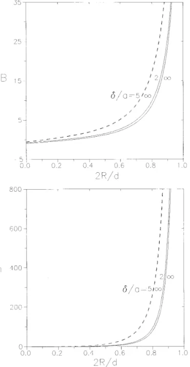
values of 2 R / d are listed in Table 1. The dependence of B and h on b0, d / a , a, h / ( h/a ) , and R / 2 d is given in Table 1 and Figs. 3 and 4. The results indicate that the particle interaction effects on the motion of two polymer-coated par-ticles can be significant.

Throughout the calculations in the previous section we have assumed a simple exponential decay of the polymer segment density. This could be an oversimplification since the convex nature of the surfaces of the particles might adjust

FIG. 3. The parameters B and h for the motion of two identical polymer-the excluded volume effects among polymer-the polymer segments. _{coated spheres with b0}_Å_{100 and U2/ U1}_{Å 0}_{1 as a function of 2 R / d in} A segment density of the following form was suggested ( 21 ) the free-draining limit ( fÅ1 ) . The solid curves are plotted for the case of aÅ0.5, and the dashed curves are plotted for the case of aÅ0.25. to allow for curvature effects on polymer distribution:

(11)

r( yi)Å0 if yi údi. [ 43b ]

For this profile in the free-draining limit, bi( yi) has the form

of Eq. [ 43 ] with ri 0replaced by bi 0 and it can be shown

that Ai` Å10b01 / 2i 0 tanh b1 / 2i 0 , [ 44a ] Bi` Å 0 1 Ai`bi 0 ( 1 0sech b1 / 2 i 0 ) 2 . [ 44b ]

It can be found that the value of Ai`is about six times greater

FIG. 4. The parameters B and h for the motion of two identical polymer-coated spheres with U2/ U1Å 01 as a function of 2 R / d . The solid curves are plotted for the case of b0Å10, and the dashed curves are plotted for the case of b0Å100. Note that d / ar `represents the free-draining limit ( fÅ1 ) and the two dashed curves are almost indistinguishable.

These calculations, which are plotted in Fig. 5 for the case of U2/ U1 Å 01, indicate that the magnitudes of B and h decrease with the increase of s for various values of 2 R / d as one would expect.

One may wish to consider a polymer segment distribution that has the same adsorbed amount as for the exponential distribution but is uniform over a distance from the particle surface:

FIG. 5. The parameters B and h for the motion of two identical polymer-coated spheres with the segment density distribution given by Eq. [ 42 ] , b0

Å100, and U2/ U1Å 01 as a function of 2 R / d in the free-draining limit. r( yi) Åri 0 if 0 °yi °di, [ 43a ]

(12)

can be seen that the particle interaction effect on B and h is weaker for the uniform distribution of segments over a dis-tance from the particle surface than for the exponential distri-bution of segments.

In addition to obtaining suitable approximate solutions of the quasisteady equations of motion of two polymer-coated spheres, it is desirable to know how well the predicted effects will be realized physically. Although experimental work has lagged behind the theory in this area, considerable data for two mutually interacting ‘‘bare’’ spheres are now available which indicate good agreement with corresponding solutions of the creeping motion equations (25). Once the segment density distribution in the surface polymer layer r(y) together with the dimensionless surface density parameter b0 is determined independently, one can measure the velocities and drag forces experienced by two polymer-coated spheres falling along the line between their centers in a viscous fluid for various values of the separation parameter (29) and choose the values of li

to test the theoretical analysis developed in this work. APPENDIX A

For completeness the definitions of functions Wik( ni) ,

Xik( ni) , Yik( ni) , and Zik( ni) in Eq. [19 ] are listed here.

Wik( ni)Å

∑

` nÅ2

H

[ R0 n/ 1 i Cink/R 0 n/ 3 i Dink] G 01 / 2 n ( ni) /

S

lj li

D

k [ g0 n/ 1 ij Cj nk/g0 n/ 3ij Dj nk] Gn 0ij

J

, [ A.1] Xik( ni)Å

∑

` nÅ2

H

0[ ( n 01 ) R0 n i Cink/( n 03 ) R0n/ 2i Dink] 1G01 / 2 n ( ni)/

S

lj li

D

k/ 1 g0 n/ 1 ij [ Gn 1ij FIG. 6. The parameters B and h for the motion of two identical

polymer-coated spheres with the segment density distribution given by Eq. [ 43 ] , b0

Å100, and U2/ U1Å 01 as a function of 2 R / d in the free-draining limit.

0( n 01 ) hijGn 0ij] Cj nk/

S

lj li

D

k/ 1 g0 n/ 3 ij The corresponding results for the exponential segment distribution are also

plotted for comparison.

1[ Gn 1ij 0( n03 ) hijGn 0ij] Dj nk

J

, [ A.2 ]

( if bi 0É 100 ) for an exponential distribution of segments

than for the polymer uniformly distributed over a region of

thickness di. Although Ai`is a function of bi 0for this seg- Yik( ni)Å

∑

` nÅ2

H

1

2[ n ( n01 ) R0 n0 1 i Cink

ment distribution, the ratio Ai/ Ai` or gi/ Ai` for the motion

of two polymer-coated spheres is independent of the segment _/_{( n}₀_{2 ) ( n}₀_{3 ) R}0 n/ 1 i Dink] G

01 / 2 n ( ni)

distribution, and its results have been given in Table 1 and

Fig. 2. In Fig. 6, the numerical results of parameters B and _/

S

lj li

D

k/ 2

g0 n/ 1ij

F

Gn 2ij0( n01 ) hijGn 1ij

h obtained using Eq. [ 43 ] as the segment distribution are

plotted for the case of U2/ U1 Å 01. The corresponding

results for the case of the exponential distribution of seg- _/_{( n}₀_{1 )}

S

n 2h

2

ij0mij

D

Gn 0ij

G

Cj nk

(13)

/

S

lj

li

D

k/ 2

g0 n/ 3

ij

F

» n0 2 … kÅ0 zij ÅRini 0( j0i ) d . [ A.19 ] 1 (01 ) k ( n 0k02 ) ! k ! ( n 02k03 ) ! ( n0k02 ) ! t n0 2 k0 2 ij APPENDIX B: NOMENCLATURE 1 [ ( n02k03 ) u2 ij /2£ij] 0 1

2n0 1 _a _{Stokes radius of a polymer segment ( m)}

Ai`, Bi` parameters defined by Eq. [ 29 ]

1

∑

» n … kÅ0 (01 )k ( n0k ) ! k ! ( n02k01 ) ! ( n0 k ) !t n0 2 k ij _A

i, Bi parameters defined by Eq. [ 9 ]

bj n, cj n, dj n coefficients defined by Eq. [ 20 ]

Cin, Din coefficients defined by Eq. [10 ] ( mn/ 2/ s,

1 [ ( n02k01 ) u2

ij /2£ij]

J

, [ A.7 ]

mn

(14)

Cinm, Dinm coefficients defined by Eq. [11] ( m n/ 2

/ s, z Stokes friction coefficient of a polymer segment ( kg / s )

mn

/ s )

d center-to-center distance between two hi fraction of tails as defined by Eq. [ 38 ] ui, f angular spherical coordinates about

parti-particles ( m)

ez unit vector in the z direction cle i

li di/ Ri

f parameter for the hydrodynamic

interac-tions among polymer segments defined L*j, Lj coefficients defined by Eqs. [ 30b, c ] by Eq. [1a ] m viscosity inside the polymer layer (kg/m s)

Fi hydrodynamic force exerted on particle i m_s fluid viscosity ( kg /m s )

( N ) _n_i _{cos u}_i

Finm functions of yi defined by Eq. [15 ] ( m

2

) _j _{R / d}

hydrodynamic force defined by Eq. [ 34 ]

FJ ( 0 )

j r polymer segment distribution ( m03)

( N ) _r_{i 0} _{polymer segment density in loops at the}

gi, hi parameters defined by Eq. [ 30 ] surface of particle i ( m03)

functions of yjdefined by Eqs. [ 22 ] – [ 26 ]

Gj, Hj, H*j fi ( 4 / 3 ) pa

3 r( yi)

( m) _f_{i 0} _{( 4 / 3 ) pa}3

ri 0

Gegenbauer polynomials of order n and

G01 / 2

n C Stokes stream function ( m3/ s )

degree01

2 C( O ) stream function in the outer region (m3/s)

Ki particle interaction factor defined by Eq. C( I )_i stream function in the inner region about

[ 8 ] _{particle i ( m}3

/ s )

Kij dimensionless resistance coefficients de- v_V radial cylindrical coordinate ( m)

fined by Eq. [ 33 ] _V_j _{coefficients defined by Eq. [ 28d ]}

Li effective hydrodynamic thickness of the

polymer layer on particle i defined by _{ACKNOWLEDGMENT} Eq. [ 8 ] ( m)

Li` effective hydrodynamic thickness of the _{This work was supported by the National Science Council of the Republic}

polymer layer on particle i defined by of China. Eq. [ 31] ( m)

Mij dimensionless mobility coefficients de- _REFERENCES

fined by Eq. [ 35 ]

p hydrodynamic pressure ( N /m2

) _{1. Napper, D. H., ‘‘Polymeric Stabilization of Colloidal Dispersions.’’}

pijn, qijn, sijn coefficients defined by Eq. [ 20 ] Academic Press, London, 1983.

2. Hunter, R. J., ‘‘Foundations of Colloid Science,’’ Vol. 1. Clarendon

Pn Legendre polynomial of order n

Press, Oxford, 1986.

ri radial spherical coordinate about particle

3. Roe, R. J., J. Chem. Phys. 44, 4264 ( 1966 ) .

i ( m)

4. Hesselink, F. Th., J. Colloid Interface Sci. 50, 606 ( 1975 ) .

Ri radius of particle i ( m) _{5. Scheutjens, J. M. H. M., and Fleer, G. J., J. Phys. Chem. 84, 178}

s curvature coefficient defined by Eq. [ 42 ] ( 1980 ) .

6. Fleer, G. J., Cohen Stuart, M. A., Scheutjens, J. M. H. M., Cosgrove,

Ui translational velocity of particle i ( m/ s )

T., and Vincent, B., ‘‘Polymers at Interfaces.’’ Chapman & Hall, Lon-velocity of particle j defined by Eq. [ 36 ]

U_J ( 0 )

j

don, 1993. ( m/ s )

7. Garvey, M. J., Tadros, Th. F., and Vincent, B., J. Colloid Interface

v fluid velocity ( m/ s ) _{Sci. 55, 440 ( 1976 ) .}

v( p )

velocity of polymer segments ( m/ s ) _{8. Kato, T., Nakamura, K., Kawaguchi, M., and Takahashi, A., Polym. J.}

13, 1037 ( 1981 ) .

Wik, Xik, Yik, Zik functions of ni defined by Eqs. [ A.1] –

9. Cohen Stuart, M. A., Waajen, F. H. W. H., Cosgrove, T., Vincent, B., [ A.4 ] ( m3

/ s, m2

/ s, m/ s, s01

)

and Crowley, T. L., Macromolecules 17, 1825 ( 1984 ) .

yi l

01

i ( ri 0Ri) ( m)

10. Baker, J. A., and Berg, J. C., Langmuir 4, 1055 ( 1988 ) .

z axial coordinate ( m) _{11. Koopal, L. K., Hlady, V., and Lyklema, J., J. Colloid Interface Sci.} ai ratio of loop-to-tail length scales for the 121, 49 ( 1988 ) .

12. Siffert, B., and Li, J. F., Colloids Surf. 62, 307 ( 1992 ) . polymer layer of particle i

13. Garvey, M. J., Tadros, Th. F., and Vincent, B., J. Colloid Interface bi parameters defined by Eq. [ 4a ]

Sci. 49, 57 ( 1974 ) . bi 0 parameters defined by Eq. [ 39 ]

14. Kawaguchi, M., and Takahashi, A., Adv. Colloid Interface Sci. 37, 219 gj coefficients defined by Eq. [ 28a ] _{( 1992 ) .}

di length scale of the polymer layer sur- 15. Doroszkowski, A., and Lambourne, R., J. Colloid Interface Sci. 26, 214 ( 1968 ) .

(15)

16. Barsted, S. J., Nowakowska, L. T., Wagstaff, I., and Walbridge, D. J., 23. Anderson, J. L., and Solomentsev, Y., Chem. Eng. Commun. 148 – 150, 291 ( 1996 ) .

Trans. Faraday Soc. 67, 3589 ( 1971 ) .

24. Gluckman, M. J., Pfeffer, R., and Weinbaum, S., J. Fluid Mech. 50, 17. Varoqui, R., and Dejardin, P., J. Chem. Phys. 66, 4395 ( 1977 ) .

705 ( 1971 ) . 18. Stromberg, R. R., Tutas, D. J., and Passaglia, E., J. Phys. Chem. 69,

25. Happel, J., and Brenner, H., ‘‘Low Reynolds Number Hydrodynam-3955 ( 1965 ) .

ics.’’ Martinus Nijhoff, Dordrecht, The Netherlands, 1983. 19. Lee, J. J., and Fuller, G. G., J. Colloid Interface Sci. 103, 569 ( 1985 ) .

26. Baker, J. A., Pearson, R. A., and Berg, J. C., Langmuir 5, 339 ( 1989 ) . 20. Barnett, K. G., Cosgrove, T., Vincent, B., Burgess, A. N., Crowley, _{27. Keh, H. J., and Tseng, Y. K., AIChE J. 38, 1881 ( 1992 ) .}

T. L., King, T., Turner, J. D., and Tadros, Th. F., Polymer 22, 283 _{28. Gerald, C. F., and Wheatley, P. O., ‘‘Applied Numerical Analysis,’’}

( 1981 ) . _{5th ed. Addison-Wesley, Reading, MA, 1994.}

21. Anderson, J. L., and Kim, J., J. Chem. Phys. 86, 5163 ( 1987 ) . 29. Steinberger, E. H., Pruppacher, H. R., and Neiburger, M., J. Fluid Mech. 34, 809 ( 1968 ) .