ELSEVIER
Available online at
www.sciencedirect.com__
computers &
, , , = , , - . , = - ( ' - ~ ) o , . . c T - m a t h e m a t i c swith applications Computers and Mathematics with Applications 51 (2006) 1075-1092
www.elsevier.com/locate/eamwa
D a t a Mining for the Diagnosis
of T y p e II D i a b e t e s from
T h r e e - D i m e n s i o n a l B o d y Surface
A n t h r o p o m e t r i c a l Scanning D a t a
C H A O - T O N S u D e p a r t m e n t of I n d u s t r i a l E n g i n e e r i n g a n d E n g i n e e r i n g M a n a g e m e n t N a t i o n a l T s i n g H u a University, Hsinchu, T a i w a netsu©mx, nthu. edu. t w
CHIEN-HSIN YANG
D e p a r t m e n t of I n d u s t r i a l E n g i n e e r i n g a n d M a n a g e m e n t N a t i o n a l C h i a o T u n g University, Hsinchu, T a i w a nKUANG-HUNG Hsu
D e p a r t m e n t of H e a l t h C a r e M a n a g e m e n t C h a n g G u n g University, T a o - Y u a n , T a i w a n W E N - K O C H I U D e p a r t m e n t of I n d u s t r i a l Design C h a n g G u n g University, T a o - Y u a n , T a i w a n(Received February 2005; revised and accepted August 2005)
A b s t r a c t - - D i a b e t e s mellitus has become a general chronic disease as a result of changes in cus- tomary diets. Impaired fasting glucose (IFG) and fasting plasma glucose (FPG) levels are two of the indices which physicians use to diagnose diabetes mellitus. Although this is a fairly accurate approach, the tests are expensive and time consuming. This study a t t e m p t s to construct a prediction model for Type II diabetes using anthropometrical body surface scanning data. Four d a t a mining approaches, including backpropagation neural network, decision tree, logistic regression, and rough set, were used to select the relevant features from the data to predict diabetes. Accuracy of clas- sification was evaluated for these approaches. The result showed t h a t volume of trunk, left thigh circumference, right thigh circumference, waist circumference, volume of right leg, and subjects' age were associated with the condition of diabetes. The accuracy of the classification of decision tree and rough set was found to be superior to t h a t of logistic regression and backpropagation neural network. Several rules were then extracted based on the anthropometrical data using decision tree. The result of implementing this method is not only useful for the physician as a tool for diagnosing diabetes, but it is sophisticated enough to be used in the practice of preventive medicine. (~) 2006 Elsevier Ltd. All rights reserved.
K e y w o r d s - - D a t a mining, Type II diabetes, Backpropagation neural network, Diagnosis.
This research was supported in part by Grant No. 93-2213-E-007-110 from National Science Council (Taiwan). The authors would like to t h a n k the medical staff at the Department of Health Examination at Chang Gung Memorial Hospital, Taiwan. We are grateful to the Chang Gung Biomedical Research Team members who provided the data and shared their experiences of medical research with us.
0898-1221/06/$ - see front matter (~) 2006 Elsevier Ltd. All rights reserved. Typeset by .Ah/tS-TEX doi: 10.1016/j.camwa.2005.08.034
1076 C.-T. S u e t al.
1. I N T R O D U C T I O N
Diabetes mellitus (DM) is a major chronic disease, affecting up to 3% of the population in industrialized countries. There are approximately 135 million people suffering from DM, and the number will rise to 300 million, or 5.4% of world population by 2025. Consequently, researchers all over the world are now paying more attention to the diagnosing a n d / o r predicting of DM.
According to the definition from the Canadian Diabetes Association [1], diabetes mellitus is a condition in which the body either cannot produce insulin or cannot effectively use the insulin it produces. Diabetes mellitus is divided into two types: T y p e I diabetes and Type II diabetes. T y p e I diabetes (or insulin-dependent diabetes, IDDM) occurs when the pancreas no longer produces any or very little insulin. The body needs insulin to use sugar as an energy source. It usually develops in childhood or adolescence and affects 10% of people with diabetes. Different from Type I, Type II diabetes (or non-insulin-dependent diabetes, NIDDM) occurs when the pancreas does not produce enough insulin to meet the b o d y ' s needs or the insulin is not metabolized effectively. Type II usually occurs later in life and affects 90% of people with diabetes.
In the past a statistical approach, such as analysis of variable (ANOVA), multi variable analysis, and factor analysis, was used to predict DM. For instance, K i m et al. [2] investigated the asso- ciation between microalbuminuria and the insulin resistance syndrome, independent of Type II diabetes, using a multiple regression analysis and multiple logistic regression analysis. The result shows t h a t the body mass index (BMI) and waist hip ratio (WHR) are both important factors for DM. Chen et al. [3] studied the association of hypertension and insulin-related metabolic syn- drome in nondiabetic Chinese using factor analysis. The result of their study shows a significant association between hypertension and the insulin-related metabolic syndrome. However, a simple statistical approach such as logistic regression cannot clearly explain the relationship among the input variables and DM. On the other hand, artificial intelligence (AI) could be a good candidate to avoid this problem. Since the early 1990s, feedforward artificial neural networks have been used increasingly in various fields, such as backpropagation for clinical diagnosis [4-6] and self- organizing map breast cancer clustering [7]. Other algorithms, like genetic algorithms, genetic programming, evolution strategies, evolutionary programming, classifier systems, and hybrid sys- tems are being reported continuously [8]. In addition, two indices, sensitivity and specificity, are used to evaluate the prediction models when conducting epidemiological studies using the statis- tical method [9-11]. In practice, we can understand t h a t researchers do not use statistics-based analysis due to the fact it may face some limitations. However, AI studies put emphasis on the accuracy of classification rather than on sensitivity and specificity. Although biochemical examination is a general approach for the diagnosis of diabetes, it has some disadvantages as a diagnostic for DM. Repeated diagnoses can lead to increased inconvenience for both the physician and the patient. On the other hand, some studies [12,13] have shown t h a t there is a relationship between body composition and DM. Based on this we use four d a t a mining approaches to find the relationship of anthropometrical d a t a and diabetes mellitus. It is our intention to provide a new diagnostic approach for physicians to diagnose DM, and thereby reduce government expenditures and enhance the health for all citizens.
The remainder of this paper is organized as follows. In Section 2, we introduce the four data mining techniques and their procedures. Methods and results are presented in Section 3. Technical and medical discussions are provided in Section 4. Finally, we draw our conclusion and make suggestion from this study in Section 5.
2. S E L E C T E D D A T A M I N I N G A P P R O A C H E S
Diagnosis is the process of selectively gathering information concerning the health status of a patient, and interpreting this information based on previous knowledge, as evidence for or against the presence or absence of a disorder [14]. Feature selection has always been one of the
processes for diagnosis and prognosis [15]. Some tools, like neural network and decision tree, are helpful for analyzing the results of feature selection. Logistic regression is also a traditional tool in many medical researches, including the process of feature selection. As for rough set, it is good at processing large and vague data where the character of the data is consistent with general medical data.
2.1. N e u r a l N e t w o r k
Neural network is one of the methods of artificial intelligence. It is characterized by (1) its pattern of connections between the neurons,
(2) its method of determining the weights of these connections, and (3) its activation function.
A neural net consists of a large number of simple processing elements called neurons. Similar to neural systems, each neuron is connected to other neurons by means of directed communication links, each with an associated weight, with the weights representing the level of information. Each neuron has an internal state, called its activation, which is a function of the inputs it has received. Typically, a neuron sends its activation as a signal to several other neurons. It is important to note that a neuron can send only one signal at a time, although t h a t signal is broadcast to several other neurons. In addition, it is convenient to visualize neurons as being arranged in layers. Typically, neurons in the same layer behave in the same manner. A multilayer net generally is composed of one input layer, hidden layers, and an output layer [16]. Usually, a neural network with signal hidden layer can provide a good performance of classification and prediction.
Neural network systems are divided into two groups: supervised learning and unsupervised learning. Backpropagation neural network is a typical network of supervised learning, and very useful for selecting features. The multilayer network modeling is accomplished via two phases: the training and the testing process. Even though it can basically approximate any function, the neural network method still has a few problems such as time consuming convergence, overfitted training, high complexity in computation and black boxes in the training results [17]. Some developed algorithms [18,19] reported that a suitable pruning of some of the input nodes might be helpful for rule extracting and knowledge acquisition.
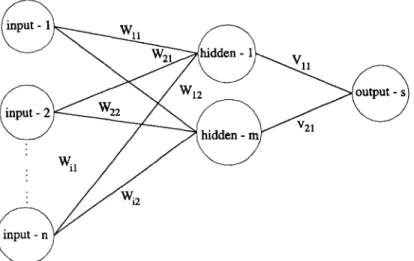
Consequently, we refer to S u e t al. [20] concerning an algorithm of feature selection. As per their research, a neural network is shown in Figure 1. This neural network is a multilayer perceptron. It is composed of a single input layer with n input nodes, a single hidden layer with m hidden
. 2 1
1078 C.-T. S u e t al.
nodes, and a single output layer with s output nodes. The connection (weight) of input to hidden is W; another hidden to output is V. The relationship between the two layers is determined by weight. It is important to note t h a t the priorities of these input nodes are according to W and V: As a result of not all of the connections being identical, i.e., sometimes W is greater than V and sometimes it is not. The priority of the input nodes is determined by Pi which is defined as follows,
Pi = IWij × V~kl, (1)
i=1 j = l k = l
where
Wiy is the weight between the ith input node and the jth hidden node; ~ k is the weight between the jth hidden node and the k th output node;
P~ is the sum of absolute multiplication values of the weights Wij and Vjk.
For the sake of convenience for the user, we calculate the mean of total Pi to determine the important input nodes according to equation (1). Thus, the ith input node is found to be an important node which will be selected if Pi >~ m e a n or else will be removed if Pi < m e a n .
In s u m m a r y of the above, we illustrate an algorithm for feature selection as follows. 2.1.1. A l g o r i t h m
Step 1: Calculate the product (Pi) of the connection of input-hidden and hidden-output for each input node.
Step 2: Sort the products and compute the mean of total Pi.
Step 3: Remove input node if its product (Pi) is less than the value of the mean of total Pi. Step 4: Go to Step 1 till the number of input nodes that are users is as expected.
2.2. D e c i s i o n T r e e
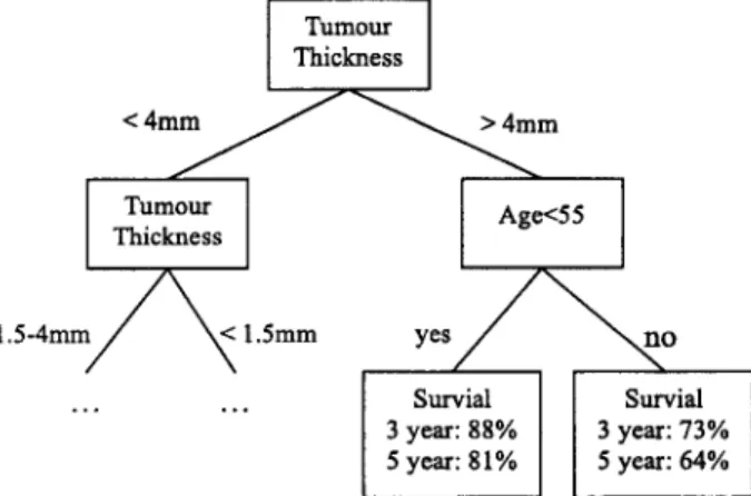
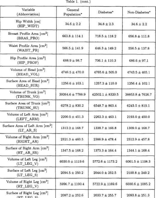
A decision tree is another feature selection approach. It is a popular classifier in machine learning applications and is also used as a diagnostic model in medicine. Decision tree is connected via nodes and branches. The tree construction process is heuristically guided by choosing the 'most informative' attribute at each step, aimed at minimizing the expected number of tests needed for classification. Let E be the entire initial set of training examples, and cl, . . . , c g be the decision classes. A decision tree is constructed by repeatedly calling a tree construction algorithm in each generated node of the tree. Tree construction stops when all examples in a node are of the same class, or if some other stopping criteria are satisfied. In brief, a decision tree is a flow-chart-like tree structure, in which each internal node denotes a test on an attribute, each branch represents an outcome of the test, and leaf nodes represent classes or a class distribution. The topmost node in a tree is the root node [21]. A typical decision tree is shown in Figure 2.
[ Turn°ur
ThicknessI
1 . 5 - 4 m m ~ < 1.5ram y e s / ~ ~ n o
Survial Survial 3 year: 88% 3 year: 73% 5 year: 81% 5 year: 64%
C4.5 is a well-known decision tree construction software (C5.0 is its recent upgrade), that is widely used, and has been incorporated into medical d a t a mining tools. Quinlan [22] provides ID3 (interactive dichotomizer 3) using a tree representation. It is an entropy-based algorithm used for some of the larger database analysis either consisting of string d a t a or integer data. Also, its interpretability has been maximized. It is important to note t h a t C4.5 is more interpretable than neural networks. C4.5 is easy to use for users with little or no knowledge of statistics and machine learning. Compared with C4.5, the C5 version classifies more accurately, much faster and requires
less memory. Although there are all these advantages, overfitting remains an important issue to overcome for the knowledge miner.
CART is another decision tree popular for data mining. Different from C4.5, CART is a binary tree based on the Gini Index (GI) to determine the condition for constructing the tree [23]. Both CART and C4.5 need to prune the initial tree after training and testing. The difference in pruning conditions between these two algorithms is t h a t C4.5 is based on the subtree, while CART is based on the entire tree. In addition, both C A R T and C4.5 rely on the specific 'cost function' to decrease the probability of misclassification [9].
In this study, entropy-based trees [24] have been chosen to analyze and induct this medical diagnostic tree. Some of the medical information such as the s y m p t o m of some diseases, or the classification of body size are vague and difficult to distinguish in a clinical diagnosis. It is worth noting here that CART is not suited for this study because it is an absolute binary classifier. In short, the entropy-based tree using C5 with not only a friendly interface, but also using a flow- chart-like structure makes it more user-friendly. The procedure, i.e., hypothesis and algorithms of entropy-based tree is as follows.
HYPOTHESIS. Let's take a training set S. Ci C S, Vi = 1 , 2 , 3 , . . . ,n. The number of class is
freq (Ci, S). IS[ is the total number of training sets. Hence, the probability of occurrence of the number of class is (freq ( C,, S) ) / I S I .
A L G O R I T H M S .
Step 1: Measure the information ( - log2(freq (Ci, S)/ISI)) of each class. Step 2: Calculate the mean information of training set S.
info(S) = - f i freq (Ci, S) //freq (Ci, S ) )
i=1 [SI l°g2 \ ISI (2)
Step 3: Partition S into S~ base on attribute A, i.e., let {$1, $2, $ 3 , . . . , Sn} E S. Step 4: Calculate the information which is partitioned.
infoA(S) = ~-~ n-~ x info(Si) (3)
i = l
Step 5: Compute the information gain.
gain (A) = info(S) - infoA(S) (4)
The algorithm computes the information gain of each attribute. The attribute with the highest information gain is chosen as the test attribute for the given set S. A node is created and labeled with the attribute, branches are created for each value of the attribute, and the samples are partitioned accordingly.
2.3. Logistic Regression
Logistic regression is a typical statistical approach which is good at binary d a t a analysis. For example, some medical research, as a result of output such as survivals (yes or no) and disease
1080 C.-T. S U e t al.
(positive or negative) are categorical data, where logistic regression is a useful analysis approach. Also accuracy of classification could satisfy some researchers and clinical operators. Different from traditional simple regression, it is a nonlinear approach to analyze the dependent variable that is categorical, such as binary data.
To obtain the logistic model from the logistic function, we write z as the linear sum a plus ~1 times X1 plus/32 times X2, and so on to flk times Xk, where the X are independent variables of interest and c~ and/3~ are constant terms representing unknown parameters. In essence, then, z is an index t h a t combines the X ' s (see equation (5)).
z = ~ + ~1X1 + ~2X2 + - . . + ~kXk. (5)
We now substitute the linear sum expression for z in the right-hand side of the formula for
f ( z ) to get the expression f ( z ) equals 1 over 1 plus e to minus the quantity a plus the sum of ~ X ~ for i ranging from 1 to k (see equation (6)),
1 1
f ( z ) - 1 + e - z - 1 + e - ( ~ + ~ x O " (6) Actually, to view this expression as mathematical model, we must place it in an epidemiologic context. Suppose we have observed independent variables X1, )(2, and so on up to Xk on group of subjects, for whom we have also determined disease status, as either 1 if "with disease" or 0 if "without disease".
We with to use this information to describe the probability t h a t the disease will develop, in a disease-free individual with independent variable values X1, X2, up to X k . The probability being modeled can be denoted by the conditional probability statement as follows,
P ( D = 1 I X I , X 2 , . . . , X k ) .
The model is defined as logistic if the expression for the probability of developing the disease, given the X is 1 over 1 plus e to minus the quantity ~ plus the sum from i equals 1 to k of /~i times X i . The terms ~ and fli in this model represent unknown parameters that we nee to estimate based on data obtained on the X ' s and on D (disease outcome) for a group of subjects. For notational convenience, we denote the probability statement P ( D = 1 ] X1, X 2 , . . . , Xk) as simply P ( X ) where the bold X is a shortcut notation for the collection of variables XI through Xk,
P ( X ) = P ( D = 1 I X 1 , X2 . . . Z k ) . (7) Thus, the logistic model [25] may be written as equation (8),
1
P ( X ) = 1 + (8)
2.4. R o u g h S e t
The rough set theory was proposed by Pawlak in 1982, and provides a mathematical tool for representing and reasoning about vagueness and uncertainty. T h e notion of indiscernibility plays an important role in this theory. Rough set theory is good at d a t a deduction, i.e., elimination of superfluous data, discovery of data dependencies, estimation of the significance of data, and the discovering of cause-effect relationships. Based on the above, rough set provides a powerful function for physicians and in medical studies as a diagnosis tool for some diseases.
The rough set theory has many important advantages [261 which are as follows, (1) provides efficient algorithms for finding hidden information in data, (2) finds minimal sets of data,
(3) evaluates the significance of data,
(4) generates minimal sets of decision rules from data, (5) easy to understand, and
According to the rough set theory, we should find the indiscernibility. Formally, let U be a set of training objects, A be a set of attributes describing the objects, C be a set of classes ^ (i) represents the value of attribute Aj for the ith and Vj be a value domain of an attribute
Aj. vj
object Obj (i). Obj (i) and Obj (k) are said to have an indiscernibility relation with attribute Aj while Obj (i) and Obj (k) have the same value of attribute Aj. Also, if Obj (i) and Obj (k) have the same values for each attribute in subset B of A, Obj (i) and Obj (k) are also said to have an indiscernibility relation with attribute set B.
The lower approximation and upper approximation are defined as
B.(X)
andB*(X)
respec- tively, as follows,B,(X) = {x I~ e U, B(x) c X } ,
B*(X) = {x I x E U, and B(x) n X # ¢}.
(9)
(10)
After the lower and the upper approximation have been found, the rough set theory can be used to derive both certain and uncertain information, and induce certain and possible rules from them.2.5. A c c u r a c y
Three accuracy indices are used to evaluate medical models. For data mining researches, accuracy of classification is often used. The other two indices, 'sensitivity' and 'specificity' are always used in epidemiological studies. For a two class problem the accuracy of classification can be estimated as
P/(P + N)
or ( P + 1 ) / ( P + N + 2) where P is the number of positive examples and N is the number of negative examples of the selected class. However, it is practical for four subsets to be considered.True positives (TP): true positive answers of a classifier denote the correct classification of positive cases.
True negatives (TN): true negative answers denote the correct classification of negative cases. False positives (FP): false positive answers denote the incorrect classification of negative
cases into a class positive.
False negatives (FN): false negative answers denote the incorrect classification of positive cases into a class negative.
According to the above definitions, the classification accuracy measures the proportion of correctly classified cases as follows,
T P + TN
Accuracy of Classification = T P + FN + TN + FP" (11) Regarding the other indices, sensitivity measures the fraction of positive cases that are classified as positive, and specificity measures the fraction of negative cases classified as negative. In other words, sensitivity can be viewed as a detection rate that one wants to maximize, while specificity can be seen as a false alarm rate which one wants to maximize.
3. I M P L E M E N T A T I O N
3.1. E q u i p m e n t s a n d M a t e r i a l s
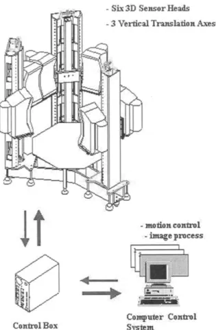
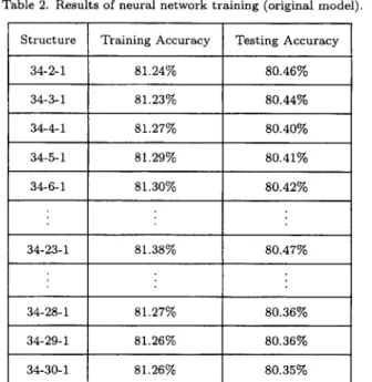
3.1.1. T h r e e - d i m e n s i o n w h o l e b o d y s c a n n e r
A three-dimension whole body scanner system (Figure 3) with six 3D sensor heads mounted on three vertical scanning mechanisms that could be motion synchronized, was used in this study. Based on optical triangulation techniques, including a CCD (charge coupled devices) image plane
1082 C.-T. Su et al.
t
:Co,tirol Box
- Six 3 D :Sensor Heads
- 3 Vertical Trauslafion Axes
. motion conlrol: ::-:image process
L~ ~
C o ~ p u l e r Control
Figure 3. A three-dimension whole study system.
O ~ j ~ 1
~
~
,
,,r m,vd
l,,:tsor C'CD
Figure 4. The optical triangulation techniques of whole body scanner.
(a 768 x 492 pixel a r r a y a n d laser sheet), six l a t e r a l laser p r o j e c t i o n s were f o r m e d (Figures 4 a n d 5). A f t e r w a r d s these six p r o j e c t i o n s n e e d e d to be merged. A t o t a l of a b o u t 280 m e a s u r e m e n t results were collected from t h e scan d a t a w i t h i n 24 seconds. In o r d e r to ensure a c c u r a c y of m e a s u r e m e n t , t h e s u b j e c t s were asked to e x t e n d t h e i r a r m s 30 ° o u t from t h e i r bodies. If t h e r e was a n y fault in this check, t h e n t h e s u b j e c t s were r e m e a s u r e d .
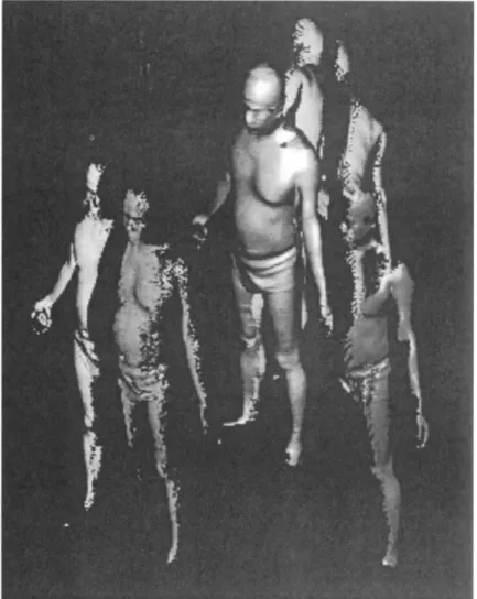
Figure 5. Six laser lateral projectors and a merged whole body.
3.1.2. Subjects
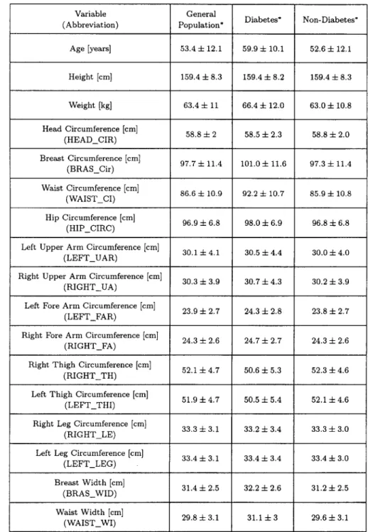
A total of 7020 subjects (3435 men and 3585 women) were recruited via the Department of Health Examination from those seeking an annual physical health check-up at Chang Gung Memorial Hospital in Tao-Yuan, Taiwan. Thirty-two anthropometrical data were measured by the whole body scanner. These data included: height, weight, head circumference, breast cir- cumference, waist circumference, hip circumference, left upper a r m circumference, right upper arm circumference, left fore a r m circumference, right fore arm circumference, right thigh circum- ference, left thigh circumference, right leg circumference, left leg circumference, breast width, waist width, hip width, breast profile area, hip profile area, volume of head, surface area of head, volume of trunk, surface area of trunk, volume of left arm, surface area of left arm, volume of right arm, surface area of right arm, volume of left leg, surface of left leg, volume of right leg, surface area of right leg. In addition to these measurements, the subjects' age and gender were collected as well.
3.2. Data Preprocessing
Some of this anthropometrical data tended to be incomplete and inconsistent, so we needed to perform data cleaning prior to implementation. D a t a cleaning tasks were carried out as follows. (1) Missing value. We ignored some missing tuples as a result of t h a t occupies a few propor-
1084 C.-T. S u e t al. (2) N o i s y d a t a . S o m e r e p e a t e d d a t a (e.g., r e p e a t e d k e y - i n b y o p e r a t o r ) w a s d e l e t e d . T h e d a t a w i t h k e y - i n e r r o r w a s also d e l e t e d . (3) I n c o n s i s t e n t d a t a . S o m e t u p l e s w e r e w i t h o u t a r e c o r d o f b i o c h e m i c a l e x a m i n a t i o n , b u t w e r e i n t h e a n t h r o p o m e t r i c a l d a t a b a s e . W e d e l e t e d i t as well. A f t e r d a t a p r e p r o c e s s i n g , 6023 s u b j e c t s ( 2 9 4 7 m e n a n d 3 0 7 6 w o m e n ) w e r e r e t a i n e d . T h e s u m m a r y of t h e s e s u b j e c t s is s h o w n i n T a b l e 1. F o u r a p p r o a c h e s , n e u r a l n e t w o r k , d e c i s i o n t r e e , l o g i s t i c r e g r e s s i o n a n d r o u g h s e t s a n a l y s i s w e r e p e r f o r m e d .
Table 1. Comparison of feature of all the included subjects with non-DM.
Variable (Abbreviation) Age [years] Height [cm] Weight [kg] Head Circumference [cm] (HEAD_ClR) Breast Circumference [cm] (BRAS_Cir) Waist Circumference [cm] (WAIST_CI) Hip Circumference [cm] (HIP_CIRC)
Left Upper Arm Circumference [cm] (LEFT_UAR)
Right Upper Arm Circumference [cm]
(RIGHT_UA)
Left Fore Arm Circumference [cm]
(LEFT_FAR)
Right Fore Arm Circumference [cm] (RIGHT_FA)
Right Thigh Circumference [cm] (RIGHT_TH) General Population* 53.4 4- 12.1 159.4 4- 8.3 63.4 4- 11 58.8 4- 2 97.7 4- 11,4 86.6 4- 10.9 96.9 4- 6.8 30.1 4- 4.1 30.3 ± 3.9 23.9 4- 2.7 24.3 4- 2.6 Diabetes* 59.9 4- 10.1 159.4 4- 8.2 66.4 4- 12.0 58.5 4- 2.3 101.0 + 11.6 92.2 4- 10.7 98.0 4- 6.9 30.5 4- 4.4 30.7 4- 4.3 24.3 4- 2.8 24.7 4- 2.7 52.1 4- 4.7 50.6 4- 5.3
Left Thigh Circumference [cm] 51.9 4- 4.7 50.5 4- 5.4 (LEFT_THI)
Right Leg Circumference [cm] 33.3 4- 3.1 33.2 4- 3.4 (RIGHT LE)
Left Leg Circumference [cm] 33.4 4- 3.1 33.4 4- 3.4 (LEFT_LEG) Breast Width [cm] 31.4 4- 2.5 32.2 4- 2.6 (BRAS_WID) Waist Width [cm] 29.8 4- 3.1 31.1 4- 3 (WAIST_WI) Non-Diabetes* 52.6 4- 12.1 159.4 4- 8.3 63.0 4- 10.8 58.8 4- 2.0 97.3 4- 11.4 85.9 4- 10.8 96.8 4- 6.8 30.0 4- 4.0 30.2 4- 3,9 23.8 4- 2.7 24,3 4- 2.6 52.3 4- 4.6 52.1 + 4.6 33.3 4- 3.0 33.4 4- 3.0 31.2 4- 2.5 29.6 4- 3.1
Variable (Abbreviation) Hip Width [cm]
(HIP_WIDT) Breast Profile Area [cm 2]
(BRAS PRO) Waist Profile Area [cm 2]
(WAIST PR)
Table 1. (cont.
Surface of Right Arm [cm 2] (RT AR SR) General Population* 34.6 =i= 2.2 663.8 =t= 114.1 Diabetes* 34.8 4- 2.3 718.5 4- 118.2 Non-Diabetes* 34.6 + 2.2 656.8 4- 111.8 556.5 4- 137.8 566.5 4- 141.9 646.3 4- 149.2
Hip Profile Area [cm 2] 688.9 4- 98.7 706.1-4- 110.3 686.6 4- 97.1 (HIP_PROF)
Volume of Head [cm 3] 4746.5 4- 470.0 4765.6 4- 505.0 4743.5 4- 465.1 ( H E A D _ V O L )
Surface Area of H e a d [cm 2] 1256.6 4- 103.1 1257.3 4- ii0.0 1256.4 4- 102.1 ( H E A D S U R )
V o l u m e of T r u n k [cm 3] 39264.6 4- 7788.9 42502.1 4- 8320.5 38853.8 4- 7626.7 ( T R U N K _ V O )
Surface Area of XYunk [cm 2] 6278.2 =t= 830.2 6548.7 4- 863.4 6243.5 =f= 819.1 (TRUNK_SU)
Volume of Left Arm [cm 3] 2200.5 4- 451.3 2262.3 4- 463.1 2193.0 4- 450.0 ( L E F T A R M )
Surface Area of Left Arm [cm 2] 1312.2 4- 168.7 1338.7 4- 166.8 1309.0 4- 168.7
(LT_AR_S)
Volume of Right Arm [cm 3] 2321.3 -4- 460.5 2388.9 4- 478.4 2312.9 4- 457.8 (RIGHT_AR)
1347.5 4- 168.2 1373.3 4- 164.4 1344.1 4- 168.4
Volume of Left Leg [cm 3] 6030.0 -4- 1119.6 5772.6 4- 1173.2 6061.5 q- 1108.3 (LT_LEG_V)
Surface of Left Leg [cm 2] 2094.5 -i- 250.2 2044.0 4- 252.5 2100.8 4- 249.2 (LT_LEG_S)
Volume of Right Leg [cm 3] 5996.7 4- 1100.4 5722.9 4- 1169.6 6030.6 4- 1085.2 (RT_LEG_V)
Surface of Right Leg [cm 2] 2087.2 4- 252.6 2033.7 4- 255.7 2093.8 4- 251.3 ( R T L E G _ S )
3.3. I m p l e m e n t a t i o n R e s u l t s
A t o t a l of 6000 d a t a sets w e r e s e l e c t e d r a n d o m l y f r o m t h e o r i g i n a l d a t a b a s e v i a d a t a pre- p r o c e s s i n g . T h e y w e r e d i v i d e d i n t o t w o g r o u p s : 80% of t h e cases w e r e t h e t r a i n i n g s e t s a n d t h e o t h e r s were t h e t e s t i n g sets, i.e., t h e t r a i n i n g sets w e r e 4800 t u p l e s a n d t h e t e s t i n g s e t s w e r e 1200 t u p l e s .
3 . 3 . 1 . N e u r a l n e t w o r k
All of t h e a n t h r o p o m e t r i c a l d a t a as well as t h e s u b j e c t s ' age a n d g e n d e r a r e t h e i n p u t n o d e s . O n e o u t p u t n o d e r e p r e s e n t s if t h e s u b j e c t suffer f r o m D M . So, t h e s t r u c t u r e of t h i s n e u r a l n e t w o r k c o u l d b e e x p r e s s e d as 3 4 - X - 1 w h e r e X d e n o t e s t h e n u m b e r of h i d d e n n o d e s . I n t h i s s t u d y , P r o f e s s i o n a l II P l u s s o f t w a r e [27] was u s e d t o p e r f o r m t h e c o m p u t a t i o n t o o b t a i n t h e s t r u c t u r e w i t h t h e m a x i m u m c l a s s i f i c a t i o n r a t e . I n t h i s m u l t i l a y e r n e u r a l n e t w o r k , n o d e s f r o m t h e h i d d e n layer, f r o m 1 to 30, w e r e chosen. T h e o t h e r p a r a m e t e r s , like m o m e n t u m w e r e set at
1086 C.-T. Suet al.
Table 2. Results of neural network training (original model). Structure Training Accuracy Testing Accuracy
34-2-1 81.24% 80.46% 34-3-1 81.23% 80.44% 34-4-1 81.27% 80.40% 34-5-1 81.29% 80.41% 34-6-1 81.30% 80.42% : : : 34-23-1 81.38% 80.47% : : : 34-28-1 81.27% 80.36% 34-29-1 81.26% 80.36% 34-30-1 81.26% 80.35%
Table 3. Results of neural network training (reduced model). Structure Training Accuracy Testing Accuracy
12-23-1 80.68% 80.15%
0.9, 0.8, and 0.7, the learning rate was set at 0.1, 0.2, and 0.3, and the number of iterations was set at 20,000. After trial and error, the accuracy of the classification of the training set and the testing set axe shown in Table 2. T h e result shows t h a t the s t r u c t u r e 34-23-1 provides the better performance when the learning rate is 0.1 and the m o m e n t u m is 0.9. Next, the network is pruned. Based on equation 1, the mean of Pi is 1.86. T h e input nodes with Pi < 1.86 are removed from the network. After that, twelve anthropometrical factors (subjects' age, waist profile area, right thigh circumference, breast profile area, left thigh circumference, volume of trunk, volume of left leg, waist circumference, volume of right leg, waist width, head circumference, breast width) were determined. Based on these twelve factors (see Table 3), we found t h a t the performance of the reduced model was similar to the original neural network model.
3.3.2. D e c i s i o n t r e e
A decision tree with 167 branches was inducted from the whole of t h e anthropometrical data (6000 instances, 34 attributes) by See 5 software. In See 5, we place training sets with 4800 tuples and testing sets with 1200 tuples to construct the decision tree (a medical diagnostic tree). Furthermore, cost files were defined and used to reduce the probability of misclassification from positive to negative. T h e original medical diagnostic tree shows t h a t the proportion of misclassification is approximate 9.3%. T h e criterion of feature selection is to collect all of the nodes t h a t form on each layer of the medical decision trees from all t h e folds. As a result of some nodes having been repeated, a total of thirteen anthropometrical factors (height, weight, breast circumference, waist circumference, left upper a r m circumference, right thigh circumference, left circumference, breast profile area, hip profile area, volume of trunk, surface area of left arm, subjects' gender and their age) were found from the medical diagnosis tree. Next, a decision tree was inducted from these thirteen attributes, and the proportion of misclassification was raised to 9.6%.
3.3.3. L o g i s t i c r e g r e s s i o n
A logistic regression model was constructed using the SPSS V10.0 software. Being similar as the R square of a simple linear regression, a likelihood ratio test was always used to test the variance and significance of this model. Next, the Lemeshow Test was used to test the goodness of fit of this model. The result showed t h a t the likelihood ratio was 2816 and t h a t the model chi-square was significant. The goodness of fit was satisfied in our model.
Next, 4800 training sets were used to construct an original logistic regression model. The accuracy of classification from the testing sets with 1200 tuples for this model is 88.50%. Then, a total of thirteen anthropometrical factors were selected through logistic regression analysis. These significant factors were weight, head circumference, right thigh circumference, left thigh circumference, breast width, waist width, hip width, waist profile area, surface area of head, volume of trunk, surface area of trunk, volume of right leg, and subjects' age, respectively. Rather than constructing the complete logistic regression model, the reduced logistic regression model is shown as equation (12). The accuracy of classification of the reduced model is 88.57%.
y = (0.0159 x AGE) + (0.0616 x W E I G H T ) - (0.0796 x H E A D _ C I R ) - (0.2371 x R I G H T TH) + (0.0027 x B R A S _ W I D ) - (0.0672 x WAIST WI) + (0.0325 x H I P _ W I D T ) + (0.0021 x W A I S T _ P R ) - (0.0015 x H E A D SUR) + (0.0001 x T R U N K VO) - (0.0009 x T R U N K _ S U ) - (0.0002 x RT LEG_V) + 10.7055
(12)
In equation (12), we can find the three significant factors are right thigh circumference, head circumference and waist width. The other factors are not significant.
3.3.4. R o u g h S e t
According to the rough set theory, 34 attributes were reduced by the Rosetta GUI version 1.4.41 software package [28]. Two steps, data discretization and computing the minimal reducts needed to be performed. We used the entropy-based algorithm to process d a t a discretization. However, a genetic algorithm (built-in Rosetta) was used to produces a set of minimal attribute subsets (minimal reducts) that define the functional dependencies. According to the algorithms, a total of 12 anthropometrical factors including height, waist circumference, right thigh circumference, left thigh circumference, right leg circumference, left leg circumference, hip width, volume of head, surface area of head, volume of trunk, volume of right leg, and surface area of right leg were used to construct a reduced model to evaluate DM. The accuracy of the classification of the reduced model is approximate to 89%.
Table 4. Summary of feature selection of four approaches.
SEX AGE HEIGHT WEIGHT H E A D C I R BRAS_CIR
Neural Network Decision Tree
WAIST_CI ~
HIP CIRC
Logistic Regression Rough Set Total 1 3 2 2 2 2 3 0
1088 C.-T. S u e t al. Table 4. (cont.) LEFT_UAR . RIGHT_UA LEFT_FAR RIGHT_FA R I G H T _ T H * * L E F T _ T H I . . RIGHT LE LEFT_LEG BRAS_WID * WAIST_WI .
Neural Network Decision Tree HIP_WIDT
B R A S _ P R O
Logistic Regression Rough Set
WAIST_PR * * HIP_PROF "k HEAD_VOL "k HEAD_SUR T R U N K _ V O "k TRUNK_SU * LEFT_ARM * LT AR S RIGHT AR RT A R SR L T _ L E G _ V * LT_LEG_S R T _ L E G _ V * * RT_LEG_S * 1 0 0 0 4 4 1 1 1 2 Total 2 2 2 1 1 2 4 1 1 0 0 0 1 0 3 1
S u m m a r y of feature selections from four d a t a m i n i n g a p p r o a c h e s a r e shown in T a b l e 4. Each a p p r o a c h has its a l g o r i t h m or function to provide some factors which are significant. T h u s , we can calculate t h e significant n u m b e r (frequency) of t h e four a p p r o a c h e s b a s e d on their functions in the l a s t column. A t o t a l frequency as p e r these four a p p r o a c h e s shows t h a t t h e volume of t r u n k , right t h i g h circumference, a n d left t h i g h circumference are g r e a t e r t h a n t h e o t h e r a n t h r o p o m e t r i c a l factors. T h e ones following after t h a t are waist circumference, v o l u m e of right leg, a n d s u b j e c t s ' age.
3 . 3 . 5 . R u l e i n d u c t i o n
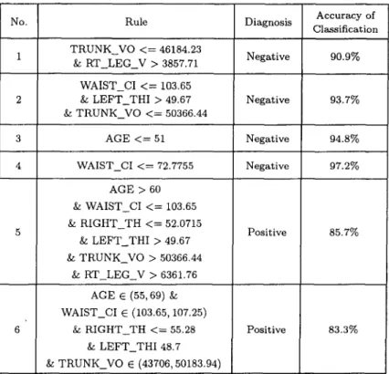
We choose six i m p o r t a n t a n t h r o p o m e t r i c a l factors including v o l u m e of t r u n k , r i g h t t h i g h cir- cumference, left t h i g h circumference, waist circumference, v o l u m e of right leg, a n d s u b j e c t s ' age as p e r Table 4 t o p e r f o r m t h e rule induction. A g a i n , See 5 was i m p l e m e n t e d a n d rules with an a c c u r a c y g r e a t e r t h a n 80% are shown in Table 5. I t is i n t e r e s t i n g to n o t e t h a t one of t h e rules was d e s c r i b e d as "if a s u b j e c t s ' age is under 51 y e a r s of age, he c a n n o t suffer from D M " .
No. 1 2 3 4 6
Table 5. Summary of accuracy of classification for rules. Accuracy of Rule Diagnosis Classification TRUNK_VO < = 46184.23
Negative 90.9% & RT_LEG_V > 3857.71
WAIST_CI < = 103.65
& LEFT_THI > 49.67 Negative 93.7% & TRUNK_VO < = 50366.44 AGE < = 51 Negative 94.8% WAIST_CI < = 72.7755 Negative 97.2% AGE > 60 & WAIST_CI < = 103.65 & RIGHT_TH < = 52.0715 & L E F T THI >49.67 & TRUNK_VO > 50366.44 & R T _ L E G V > 6 3 6 1 . 7 6 AGE E (55, 69) & WAIST_CI E (103.65, 107.25) & RIGHT_TH <-= 55.28 & LEFT_THI 48.7 & TRUNK_VO E (43706, 50183.94) Positive Positive 85.7% 83.3%
4. D I S C U S S I O N
We found the different body factors from these four d a t a mining approaches. The accuracy of the classification of the models conducted from these four approaches all exceeded 80%. The result of that is acceptable when compared with other epidemiological research. Many epidemio- logical researches often use a statistics approach, such as logistic regression, to predict a disease. However, we can't obtain the full meaning of input x to output y even though this relationship is significant via logistic regression approach. Therefore, the other approaches, i.e., neural network, decision tree and rough set were introduced in this study. The order of accuracy of these four models is decision tree, rough set, logistic regression, and with neural network the least accurate. Note that decision tree with a function of adjusting cost is helpful for the classification tasks. So, it is a principal cause that the performance of decision is greater than all the other approaches, perhaps.
In clinical practice, impaired fasting glucose (IFG) and fasting plasma glucose level (FPG) are often two predictors for diabetes mellitus. Nevertheless, there exists no accurate and precise measure for body composition. Although some researches indicate t h a t BMI and W H R are related to metabolic syndrome, hypertension, diabetes and hyperlipidemia, pure height and/or weight measure vary significantly across ethnic groups [29,30]. However, the result of this study is not restricted to BMI and WHR, i.e. height, weight, waist circumference, and hip circumference. Obviously, the artificial intelligence approach brings with it new features which are different from the traditional statistics.
Studies have reported a steady increase in the incidence of chronic diseases such as diabetes with increasing BMI. However, physicians may find some inconsistent conditions in their diagnosis. Such as with some metabolic diagnosis, a patient without obesity, i.e., although BMI in normal, he/she has been suffering from diabetes for a long time. On the other hand, some patients do not suffer from diabetes but their BMI are classed in the abnormal level. Furthermore, ethnic groups create a bias across the BMI [31-33]. Thus, the BMI seems to have limitations in the
1090 C.-T. Suet al.
interpretation of its association with diabetes. Physicians m a y risk making a misdiagnosis for diabetes if they base their assessment solely on BMI.
In practice, some research shows that body fat is related to diabetes [12,13,30]. For adults, the fat usually disperses uniformly to viscera and subcutaneous tissue. However, Erwin et al. [12] consider t h a t the subcutaneous adipose tissue in people with diabetes, especially in the lower trunk, is greater than in healthy people. Furthermore, some research shows t h a t the visceral fat is a major risk for impaired fasting glucose [29,30]. Therefore, they infer t h a t the visceral fat is a risk factor for diabetes. However, we obtained a crude index when we based on WHR, i.e., waist circumference, to evaluate visceral fat in relation to diabetes. It was relatively easy to do, even though advanced medical techniques, such as computer topography (CT) and magnetic resonance imaging (MRI) are available to evaluate visceral fat. These techniques however are much too expensive for screening all patients, and it could reduce the wish to be examined for diabetes for some patients. Thus, a simple and accurate approach is worthy of performing.
In this study, we find six factors associated with diabetes, and they are in order of impor- tance: volume of trunk, left thigh circumference, right thigh circumference, waist circumference, volume of right leg, and subjects' age. This result provides a new approach for the diagnosis of diabetes. It is not only a simple approach, but the accuracy of classification is satisfied in the diabetes diagnosis when we measure the patient's thighs. Furthermore, we m a y obtain a better performance of DM diagnostic using thighs because the body weight is almost entirely loaded on the thighs. Some studies show that patients with a metabolic syndrome such as diabetes have dimensions t h a t are greater than that of the healthy group. As anticipated, their thighs also have dimensions larger than t h a t of the healthy group. In addition, this noncontact method of making measurements may decrease some problems, such as bacterium infection. Basically, when using our approach, the evaluation of subcutaneous adipose tissue of the thigh is more accurate than the evaluation of the visceral fat at the waist. Nevertheless, this study shows t h a t the waist circumference is also an important factor, and it is consistent with previous researches [34].
5. C O N C L U S I O N
The aim of this study was to investigate what the risk factors were for anthropometrical data of Type II diabetes using four data mining approaches. Accuracy of classification was used to evaluate the performance of these four models. First, we found six factors including right thigh circumference, left thigh circumference, volume of trunk, waist circumference, volume of right leg and subjects' age to diagnose DM. Compared with the traditional approach for diagnosing DM, in particular the biochemical test, our study provides a new way with regard to anthropometry interventions, for doing that. We also found t h a t the thigh circumference is a good factor (i.e., with high weight or significance) among the anthropometrical d a t a in any one of these four approaches. It is obvious t h a t using the thigh circumference to diagnose DM is a better alternative than using BMI or WHR. Furthermore, measuring the thigh circumference can be done quickly and simply, but the 3D-whole-body-scanning procedure can reduce the discomfort of the subjects. At the same time, the accuracy of classification of all of the models was greater than 80%. This indicates t h a t all the approaches of either the statistics-based or the AI-based could provide a good performance of classification of the case. Even though each approach is founded in a strong theory, the performance of the decision tree (entropy-based) and the rough set (via indiscernibility) are still greater than the logistic regression and neural network. In addition, the decision tree with a flow-chart-like tree structure is good at interpreting the results, and is a good tool for persons who have no informatics knowledge, such as physicians. Also, the rules from the decision tree induction are helpful in a physician's diagnosis, and are also good for the prevention of DM in clinical medicine. Concerning DM diagnosis, in particular the evaluation of the risk for contracting DM using anthropometrical data such as thigh circumference, is certainly worth investigating in future study.
R E F E R E N C E S
1. Canadian Diabetes Association, Diabetes Dictionary h t t p : / / ~ . d i a b e t e s , ca, (2003).
2. Y.I. Kim, C.H. Kim, C.S. Choi, Y.E. Chung, M.S. Lee, S.I. Lee, J.Y. Park, S.K. Hong and K.U. Lee, Microalbuminuria is associated with the insulin resistance syndrome independent of hypertension and type 2 diabetes in the Korean population, Diabetes Research and Clinical Practice 52, 145-152, (2001).
3. C.H. Chen, K.C. Lin, S.T. Tsai and P. Chou, Different association of hypertension and insulin-related metabolic syndrome between man and women in 8437 nondiabetic Chinese, American Yournal of Hyper- tension 13 (7), 846-853, (2000).
4. G. Dorffner and G. Porenta, On using feedforward neural networks for clinical diagnostic tasks, Artificial Intelligence in Medicine 6, 417-435, (1994).
5. D.B. Fogel, E.C. Wasson III, E.M. Boughton and V.W. Porto, Evolving artificial neural networks for screening features from mammograms, Artificial Intelligence in Medicine 14, 317-326, (1998).
6. R. Folland, E. Hines, R. Dutta, R. Boilot and D. Morgan, Comparison of neural network predictors in the classification of tracheal-bronchial breath sounds by respiratory auscultation, Artificial Intelligence in Medicine 31, 211-220, (2004).
7. M.K. Markey, J.Y. Lo, C.D. Tourassi and C.E. Jr. Floyd, Self-organizing map for cluster analysis of a breast cancer database, Artificial Intelligence in Medicine 27, 113-127, (2003).
8. A. Carlos, R. Pena and S. Moshe, Evolutionary computation in medicine: An overview, Artificial Intelligence in Medicine 19, 1-23, (2000).
9. M. Kukar, I. Kononenko, C. Gro~elj, K. Kralj and J. Fettich, Analysing and improving the diagnosis of ischaemic heart disease with machine learning, Artificial Intelligence in Medicine 16, 25-50, (1999). 10. F. Mizoguchi, H. Ohwada, M. Daidoji and S. Shirato, Using inductive logic programming to learn classification
rules t h a t identify glaucomatous eyes, In Intelligent Data Analysis in Medicine and Pharmacology, (Edited by N. Lavra~, E. Keravnou and B. Zupan), pp. 227 242, Kluwer, (1997).
11. W.R. Shankle, S. Mani, M.J. Pazzani and P. Smyth, Dementia screening with machine learning methods, In Intelligent Data Analysis in Medicine and Pharmacology, (Edited by N. Lavra~, E. Keravnou and B. Zupan), pp. 149-166, Kluwer, (1997).
12. T. Erwin, M. Reinhard, S. Karl and R. Gilbert, The determination of three subcutaneous adipose tissue compartments in non-insulin-dependent diabetes mellitus women with artificial neural networks and factor analysis, Artificial Intelligence in Medicine 17, 181-103, (1999).
13. T. Erwin, M. Reinhard, S. Karl and R. Gilbert, Artificial neural networks compared to factor analysis for low-dimensional classification of high-dimensional body fat topography d a t a of healthy and diabetic subjects, Computers and Biomedical Research 33, 365-374, (2000).
14. P.J.F. Lucas, Analysis of notions of diagnosis, Artificial Intelligence 105 (12), 295-343, (1998).
15. P. Abdolmaleki, L.D. Buadu and H. Naderimansh, Feature extraction and classification of breast cancer on dynamic magnetic resonance imaging using artificial neural network, Cancer Letters 171 (2), 183-191,
(2ooi).
16. L. Fausett, Fundamentals of Neural Networks, Prentice-Hall International, (1994).
17. H. Tsukimoto, Extraction rules from trained neural networks, I E E E Transactions on Neural Networks 11, 377-389, (2000).
18. R. Andrews, J. Diederich and A.B. Tickle, Survey and critique of techniques for extracting rules from trained artificial neural networks, Knowledge-Based System 8, 373-389, (1995).
19. R. Andrews and J. Diederich, Rules and networks, Proceedings of Rule Extraction Trained Artificial Neural Networks Workshop, AISB, (1996).
20. C.T. Su, H.H. Hsu and C.H. Tsai, Knowledge mining from trained neural networks, Journal of Computer Information Systems 42 (4), 61-70, (2002).
21. J.W. Han and M. Kamber, Data Mining: Concepts and Techniques, Morgan Kaufmann, San Francisco, CA,
(2001).
22. J.R. Quinlan, C~.5: Programs for Machine Learning, Morgan Kaufmann, San Mateo, CA, (1993).
23. L. Breiman, J.H. Friedman, R.A. Olshen and C.J. Stone, Classification and Regression Trees, Wadsworth Int., Belmont, CA, (1984).
24. J.R. Quinlan, Induction of decision trees, Machine Learning 1 (1), 81-106, (1986).
25. D.G. Kleinbaum, Logistic regression: A self-learning text, Springer-Verlag, New York, (2002).
26. Z. Pawlak, Why rough sets, Proceedings of the Fifth IEEE International Conference on Fuzzy Systems 2, 738-743, (1996).
27. NeuralWare, NeuralWorks Professional I I / Plus getting started: A tutorial for Microsoft Windows comput- ers, Version 5.50, Carnegie, PA, (2001).
28. Rosetta GUI Version 1.4.41 h t t p : / / i d i . n t n u . n o / ~ a l e k s / r o s e t ~ ; a / , NTNU, Norway, (2001).
29. M.J. NcNeely, E.J. Boyko, J. B. Shofer, L. Newell-Morris, D.L. Leonetti and W.Y. Fujimoto, Standard definitions of overweight and central adiposity for determining diabetes risk in Japanese Americans, American Journal of Clinical Nutrition 74, 101-104, (2001).
30. H. Nagaretani, T. Nakamura, T. Funabashi, K. Kotani, M. Miyanaga, K. Togunaga, M. Takahasi, H. Nishizawa, K. Kishida, H. Kuriyama, K. Hotta, S. Yamashita and Y. Matsuzawa, Visceral fat is major contribution for multiple risk clustering in Japanese men with impaired glucose to tolerance, Diabetes Care 24, 2127-2133, (2001).
[092 C.-T. Suet al.
31. N.G. Norgan, Population difference in body composition in relation to the body mass index, European Journal of Clinical Nutrition 48 (Supplement), S10-$25, (1994).
32. J. Wang, J.C. Thornton, M. Russel, S. Burastero, S.B. Heymsfield and R.N. Pierson, Asians have lower BMI but higher percentage body fat t h a n do white: Comparison of anthropometric measurements, American Journal Clinical Nutrition 60, 23-28, (1994).
33. D. Gallagher, M. Visser, D. Sepulveda, R.N. Pierson, T. Harris and S.B. Heymsfield, How useful is BMI for comparison of body fatness across age, sex and ethic groups, American Journal of Epidemiology 143, 228-239, (1996).
34. A.H. Kissebah, D.S. Freedman and A.N. Peiris, Health risks of obesity, Medicine Clinics of North America