A Novel Approach to Comparison-Based Diagnosis for Hypercube-Like Multiprocessor Systems

全文

(1)A Novel Approach to Comparison-Based Diagnosis for Hypercube-Like Multiprocessor Systems Chieh-Feng Chiang Jimmy J. M. Tan [email protected] [email protected] Department of Computer Science, National Chiao Tung University, Hsinchu, Taiwan system but ignored some local systematic details. For example, if a system is of diagnosability t, it is at most t-diagnosable. That is, given any syndrome σ, all the faulty nodes in a system G can be precisely identified if G is with at most t faulty nodes. But it is possible to correctly point out all faulty nodes in some part of the system G under any given syndrome if G is with more than t faulty nodes. Thus, only considering the global status let us lose some local detail of a system. In this paper, we present a novel idea on system diagnosis which is called local diagnosability. More local information about a system can be retrieved through this concept. In other words, every node in a system has its own local diagnosability which states some kind of connection status around it. Moreover, we proposed a sufficient condition to easily compute the local diagnosability of each node based on the comparison model. Finally, we can get back to the original global diagnosis in the point of view of local diagnosis. We prove that the diagnosability of an n-dimensional hypercube-like network HLn is n for n ≥ 5 in this local sense, and show that the local diagnosability of each node in an n-dimensional hypercube-like network equals to its degree with up to n − 2 faulty edges.. Abstract Interconnection networks have been an active research area for parallel and distributed computer systems. The diagnosability has played an important role in the reliability of interconnection networks. In this paper, we present a novel idea on system diagnosis called local diagnosability. There is a strong relationship between the local diagnosability and the traditional global one. For this local sense, we focus more on a single processor and require only identifying the status of this particular processor correctly. We propose a sufficient condition to determine the local diagnosability of a given processor. Moreover, we prove that the diagnosability of an n-dimensional hypercube-like network HLn is n for n ≥ 5 in this local sense, and show that the local diagnosability of each node in an n-dimensional hypercube-like network equals to its degree with up to n − 2 faulty edges.. 1. Introduction. With the rapid development of technology, multiprocessor systems are more and more important. The reliability of the processors in multiprocessor systems is therefore becoming an important issue. In order to maintain the reliability of a system, if a processor is found faulty, it should be replaced by a fault-free one. The procedure of identifying all the faulty nodes is called the diagnosis of the system. The maximum number of faulty nodes that the system can guarantee to identify is called the diagnosability of the system. There are several approaches for interconnected processors to perform self-diagnosis for faulty ones. One major approach is called the comparison model, first proposed by Malek and Maeng [1] [2]. This approach performs the diagnosis by sending the same input to a pair of adjacent processors and comparing their responses. In the previous studies on diagnosis, most investigators focused on the global diagnosis ability of a. 2. Preliminaries. In this section, we give the basic of graph definition and notation [6]. G = (V, E) is a graph if V is a finite set and E is a subset of {(u, v) | (u, v) is an unordered pair of V }. The degree of node v in a graph G is the number of edges incident with v. A node cover of G is a subset Q ⊆ V (G) such that every edge of E(G) has at least one end node in Q. A node cover set with the minimum cardinality is called a minimum node cover. Vaidya et al. [5] introduced a class of hypercubelike interconnection networks, called HL-graphs, which can be defined by applying the ⊕ operation repeatedly as follows: HL0 = {K1 }; for m ≥ 1, 1. - 165 -.

(2) HLm = {G0 ⊕ G1 | G0 , G1 ∈ HLm−1 }, which has node set V (G0 ⊕ G1 ) = V (G0 ) ∪ V (G1 ) and edge set E(G0 ⊕ G1 ) = E(G0 ) ∪ E(G1 ) ∪ M , where M is an arbitrary perfect matching between the node set of G0 and G1 . That is, M is a set of edges connecting the nodes of G0 and G1 in a bijection. For the purpose of self-diagnosis of a given system, several different models have been proposed. The comparison model, called the MM model, proposed by Maeng and Malek [2] [3], is considered to be a major approach for fault diagnosis in multiprocessor systems. In this approach, for each processor w which has two distinct links to two other processors u and v, the diagnosis can be performed by sending two identical signals from w to u and from w to v, and then comparing their returning responses. Furthermore, in the MM* model [4], a special case of the MM model, it is assumed that a comparison is performed by each processor for each pair of distinct connected neighbors. This diagnosis-by-comparison strategy can be modeled as a labeled multigraph M = (V, C) , called a comparison graph, where V represents the set of all processors in G and C represents the set of labeled edges. For each labeled edge (u, v)w ∈ C, w is a label on the edge, which means that processors u and v are being compared by the comparator w. The output on a labeled edge (u, v)w ∈ C is denoted by r((u, v)w ) , which represent the comparison result of w for the two responses from u and v. An agreement is denoted by r((u, v)w ) = 0, whereas a disagreement is denoted by r((u, v)w ) = 1. If r((u, v)w ) = 1 , at least one member of {u, v, w} is faulty; or, if r((u, v)w ) = 0 and w is known to be fault-free, both u and v are fault-free. For a given syndrome σ, a subset of nodes F ⊂ V (G) is consistent with σ if the syndrome σ can be produced from the situation that all nodes in F are faulty and all nodes in V − F are fault-free. Let σF denote the set of syndromes which are consistent with F . Notice that for a syndrome σ, there might be more than one faulty subset of V which are consistent with σ. A system is defined to be diagnosable if, for every syndrome σ, an unique set of nodes F ⊆ V is consistent with it. In addition, a system is called t-diagnosable if the system is diagnosable as long as the number of faulty processors is at most t. The maximum number t for a system to be t-diagnosable is called the diagnosability of the system. Two distinct subsets of nodes F1 , F2 ⊂ V are distinguishable if and only if σF1 ∩ σF2 = φ; otherwise, F1 and F2 are indistinguishable. Let G = (V, E) be a graph and let M = (V, C) be. the comparison graph of G. Define the order graph [4] of a node u ∈ V to be Gu = (Xu , Yu ), where Xu = {v | either (u, v) ∈ E or (u, v)w ∈ C for some w} and Yu = {(v, w) | v, w ∈ Xu and (u, v)w ∈ C}. For a given node u ∈ V , the order of u is defined as the cardinality of a minimum node cover of Gu . For a subset of nodes U ⊂ V , define T (G, U ) to be the set {v | (u, v)w ∈ C and u, w ∈ U and v ∈ V − U }. The following is a lemma presented by Sengupta and Dahbura to characterize whether a system is tdiagnosable. Lemma 1. [4] For every two distinct subsets of nodes F1 and F2 , (F1 , F2 ) is a distinguishable pair if and only if at least one of the following conditions is satisfied: 1) ∃u, w ∈ V − F1 − F2 and ∃v ∈ (F1 − F2 ) ∪ (F2 − F1 ) such that (u, v)w ∈ C, 2) ∃u, v ∈ F1 − F2 and ∃w ∈ V − F1 − F2 such that (u, v)w ∈ C, or 3) ∃u, v ∈ F2 − F1 and ∃w ∈ V − F1 − F2 such that (u, v)w ∈ C. In the rest of this paper, we present our novel concept of local diagnosability under the comparison diagnosis model and discuss some properties of it.. 3. Local diagnosability. In this section, we will define the definition of local diagnosability, and we will provide some practical theorems about local diagnosability. By these theorems, we can easily check the diagnosability of a system. We now introduce the concept of a system being locally t-diagnosable at a given node. Definition 1. A system G(V, E) is locally tdiagnosable at node x ∈ V (G) if, given a test syndrome σF produced by the system under the presence of a set of faulty nodes F containing node x with |F | ≤ t, every set of faulty nodes F ′ consistent with σF and |F ′ | ≤ t, must also contain node x. An equivalent way of stating the above definition is given below. Proposition 1. A system G(V, E) is locally tdiagnosable at node x ∈ V (G) if, for each pair of distinct sets F1 , F2 ⊂ V (G) such that F1 6= F2 , |F1 |, |F2 | ≤ t, and x ∈ (F1 − F2 ) ∪ (F2 − F1 ), (F1 , F2 ) is a distinguishable pair. Then, we define the local diagnosability of a given node as follows. 2. - 166 -.

(3) Definition 2. The local diagnosability tl (x) of a node x ∈ V (G) in a system G(V, E) is defined to be the maximum number of t for G being locally tdiagnosable at x, that is,. t-diagnosable at node x by Proposition 1, which is a contradiction. 2 We now propose a substructure at node x, called an extended star, which can guarantee the local diagnosability of node x.. tl (x) = max{t | G is locally t − diagnosable at x}. The concept of a system being locally t-diagnosable at a node x is consistent with the traditional concept of a system being t-diagnosable in the global sense. The relationship between these two is as follows.. x. Theorem 1. A system G(V, E) is t-diagnosable if and only if G is locally t-diagnosable at x, for every x ∈ V (G).. v11. v21. vn1. v12. v22. vn2. v13. v23. vn3. v14. v24. vn4. Figure 1: extended star sturcture ES(x; n).. Theorem 2. The diagnosability of a system G(V, E) is t if and only if. Definition 3. Let x be a node in a graph G(V, E). For n ≤ degG (x), an extended star min{tl (x) | ∀x ∈ V (G)} = t. ES(x; n) of order n at node x is defined as ES(x; n) = (V (x; n), E(x; n)), where the set of Now, we need some definitions for further discusnodes V (x; n) = {x} ∪ {vij | 1 ≤ i ≤ sion. For any set of nodes U ⊆ V (G), G[U ] denotes n, 1 ≤ j ≤ 4} and the set of edges E(x; n) = the subgraph of G induced by the node subset U . Let {(x, vk1 ), (vk1 , vk2 ), (vk2 , vk3 ), (vk3 , vk4 ) | 1 ≤ k ≤ n}. H be a subgraph of G and v be a node in H, degH (v) denotes the degree of v in subgraph H. For a given We say that there is an extended star structure set of nodes S ⊆ V (G), we use G − S to denote the ES(x; n) ⊆ G at node x if G contains an extended induced subgraph G[V (G) − S]. Let S be a set of star ES(x; n) of order n at node x as a subgraph. nodes and x be a node not in S, we use Cx,S to deTheorem 4. Let x be a node in a system G(V, E). note the connected component which x belongs to in The local diagnosability of x is at least n if there exists G − S. The symmetric difference of two sets A and an extended star ES(x; n) ⊆ G at x. B is defined as the set A∆B = (A ∪ B) − (A ∩ B). In the following, we propose a sufficient condi- Proof. We use Theorem 3 to prove this result. First, tion for verifying whether a system G is locally t- we define lk = (vk1 , vk2 , vk3 , vk4 ) to be a quadruple of four consecutive nodes for any k, 1 ≤ k ≤ n, with diagnosable at a given node x. respect to ES(x; n). We note that lk is a path of Theorem 3. A system G(V, E) is locally t- length 3. Accordingly, the cardinality of a node cover diagnosable at a given node x ∈ V (G) if, for every of each l is at least 2. Let S ⊂ V (G) be a set of k set of nodes S ⊂ V (G), |S| = p, 0 ≤ p ≤ t − 1, and nodes in G with |S| = p, 0 ≤ p ≤ n − 1, and x ∈ / S. x∈ / S, the cardinality of every node cover including After deleting S from V (G), there are at least (n − x of the component Cx,S is at least 2(t − p) + 1. p) complete lk ’s still remaining in ES(x; n), where Proof. We prove this theorem by contradiction. the word “complete” means that all vk1 , vk2 , vk3 , Suppose G is not locally t-diagnosable at node x. By and vk4 of an lk have not been deleted in G − S. Proposition 1, there exists two distinct sets of nodes Thus, the cardinality of a node cover including x of F1 6= F2 ⊂ V with |Fi | ≤ t, i = 1, 2, and x ∈ F1 ∆F2 , the connected component Cx,S is at least 1 + 2(n − such that (F1 , F2 ) is an indistinguishable pair. Let p). Therefore, the system G with an extended star S = F1 ∩ F2 , then |S| = p, 0 ≤ p ≤ t − 1. According ES(x; n) is locally n-diagnosable at x by Theorem to the condition, the cardinality of a node cover in- 3. By Definition 2, the local diagnosability of x is at 2 cluding x of the component C is at least 2(t−p)+1. least n, i.e. tl (x) ≥ n. x,S. Since |F1 ∆F2 | ≤ 2(t − p) and x ∈ F1 ∆F2 , there is at least one node which is a member of the node cover of Cx,S lying in Cx,S − F1 ∆F2 . Consequently, there is at least one edge of Cx,S lying in Cx,S − F1 ∆F2 . Then, (F1 , F2 ) is a distinguishable pair since it satisfies condition 1 of Lemma 1. Therefore G is locally. Theorem 5. Let x be a node in a system G(V, E) with degG (x) = n. The local diagnosability of x is at most n. Proof. We prove this proposition by contradiction. Suppose on the contrary that the local diagnosability 3. - 167 -.

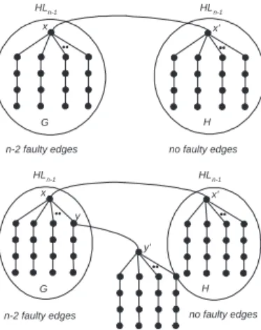
(4) of x is n + 1 or more, i.e. tl (x) ≥ n + 1. Let the nodes adjacent to x be vk , for all k, 1 ≤ k ≤ n. Let F1 be the set {x} ∪ {vk | k = 1 to n} and F2 be the set {vk | k = 1 to n}. Then, (F1 , F2 ) is not a distinguishable pair according to Lemma 1, which is a contradiction. Then, the proof is completed. 2. F2. b. X XX F1. a. Figure 2: an indistinguishable pair.. By Theorem 4 and Theorem 5, we have the followexclusive {(a, b)} are faulty. We can see that (F1 , F2 ) ing result. is an indistinghushable pair by Lemma 1. Theorem 6. Let x be a node in a system G(V, E) Now we are going to prove this theorem in the folwith degG (x) = n. The local diagnosability of x is n lowing. Suppose the local diagnosability of any node if there exists an extended star ES(x; n) ⊆ G at x. in HLn−1 with n − 3 edge faults equals to its degree . Consider HLn which has n − 2 faulty edges is constructed with two copies of HLn−1 , one is G and the 4 Diagnosability of Hypercube- other is H. Without loss of generality, we may assume that x is in G and deg(x) = m. And the degree Like Network of node x′ in H corresponding to x is m′ . We prove Theorem 7. The diagnosability of an n-dimensional it in two cases. case 1: There are k faulty edges that are crossed hypercube-like network HLn is n for n ≥ 5. edge, where 1 ≤ k ≤ n − 2. See Fig. 3. Proof. We prove this theorem by induction on n, case 1.1: Edge (x, x′ ) is faulty. the dimension of hypercube-like network HLn . Since there are k faulty edges in the crossed edge, Basis: We now prove that HL5 is 5-diagnosable. where 1 ≤ k ≤ n − 2, the number of faulty edges in Consider any node x in HL5 , we find that there is G is at most n − 3. So the local diagnosability of x in a subgraph ES(x, 5) at x. Hence node x in HL5 is G equals to its degree m. Hence there is a subgraph locally 5-diagnosable by Theorem 6. Because HL5 ES(x, m) at x in HL because (x, x′ ) is faulty. By n is node symmetric, every node in HL5 is locally 5- Theorem 6, the local diagnosability of x in HL with n diagnosable. Hence HL5 is 5-diagnosable by Theo- n − 2 faulty edges equals to its degree m . rem 1. case 1.2: Edge (x, x′ ) is fault-free. Hypothesis: Suppose the claim holds for HLn−1 . Since there are k faulty edges in the crossed edge, Induction: Consider an n-dimensional hypercube-like where 1 ≤ k ≤ n − 2, the faulty edges in G and H are network HLn . We want to show that each node at most n − 3. So the local diagnosability of x in G of HLn has a subgraph ES(x, n) at it. Consider equal to its degree m − 1 and the local diagnosability any node x in HLn , we can separate HLn into two of x′ in H equal to its degree m′ − 1. Hence there is a HLn−1 , denoted by G and H. Without loss of gensubgraph ES(x, m − 1) at x in G and ES(x′ , m′ − 1) erality, we may assume that x is in G. By hypothin H. So there is a subgraph ES(x, m) at x in HLn . esis, there is a subgraph ES(x, n − 1) in G. ConBy Theorem 6, the local diagnosability of x in HLn sider the corresponding node x′ in H, there is a subwith n − 2 faulty edges equals to its degree m. ′ graph ES(x , n − 1) in H. Hence there is a subcase 2: There are no faulty edges that are crossed graph ES(x, n) in HLn . Therefore x is locally nedge. diagnosable by Theorem 6. And HLn is node symcase 2.1: All faulty edges are in G. (That is, there metric, each node in HLn is locally n-diagnosable, are n − 2 faulty edges in G.) See Fig. 4. hence HLn is n-diagnosable by Theorem 1. 2 If there is a faulty edge s belonging to Theorem 8. If the local diagnosability of each node {(x, v11 ), (x, v21 ), ..., (x, vn1 )}, we assume that s is in HLn−1 with n − 3 edge faults equals to its degree, fault-free. Hence there are n−3 faulty edges in G. By then the local diagnosability of each node in HLn with assumption, the local diagnosability of x in G equals to its degree. So we can find ES(x, m − 1) in G. n − 2 edge faults equals to its degree. Consider x′ in H, we can also find ES(x′ , m′ − 1) Proof. First we explain why the local diagnosability in H by assumption. Therefore, we can easily find of each node in HLn does not equal to its degree if ES(x, m) in HLn . Then the local diagnosability of x there are n − 1 faulty edges. We give an example in HLn with n − 2 faulty edges equals to its degree in Fig. 2. Suppose all edges incident with node b by Theorem 6. 4. - 168 -.

(5) 5. x. G. HL n-1. x. x' y y'. H. G n-2 faulty edges. no faulty edges. Figure 4: case2.1 of the proof in Theorem 8. HL n-1. HL n-1. x. G the number of faulty edges is between 1 to n-3. x'. H the number of faulty edges is between 1 to n-3. Figure 5: case2.2 of the proof in Theorem 8.. References [1] J. Maeng and M. Malek, “A Comparison Connection Assignment for Self-Diagnosis of Multiprocessors Systems,” Proc. 11th Int’l Symp. Fault-Tolerant Computing, pp. 173-175, 1981. [2] M. Malek, “A Comparison Connection Assignment for Diagnosis of Multiprocessors Systems,” Proc. 7th Int’l Symp. Computer Architecture, pp. 31-36, 1980. [3] F. P. Preparata, G. Metze, and R. T. Chien, “On the Connection Assignment Problem of Diagnosis Systems,” IEEE Tran. Electronic Computers, vol. 16, no. 12, pp. 848-854, Dec. 1967. [4] A. Sengupta and A. Dahbura, “On SelfDiagnosable Multiprocessor Systems: Diagnosis by the Comparison Approach,” IEEE Tran. Computers, vol. 41, no. 11, pp. 1386-1396, Nov. 1992.. HL n-1 x'. k faulty edges. no faulty edges. HL n-1. [5] A. Vaidya, P. Rao, and S. Shankar, “A Class of Hypercube-Like Networks,” Proc. Fifth IEEE Symp. Parallel and Distributed Processing (SPDP), pp. 800-802, Dec. 1993.. X at most n-3 faulty edges. H. G. The reliability of interconnection networks is an important issue. The diagnosability is also an important factor in measuring the reliability of interconnection networks. In this paper, we proposed a new point of view which is called the local diagnosability, and a theorem to verify the diagnosability of multiprocessor systems under the comparison-based diagnosis model. Then we prove the diagnosability of an ndimensional hypercube-like network is n for n ≥ 5, and show that the local diagnosability of each node in an n-dimensional hypercube-like network equals to its degree with up to n − 2 faulty edges. x. x'. n-2 faulty edges. Conclusions. HL n-1. HL n-1. HLn-1. If there is a faulty edge s belonging to {(v11 , v12 ), (v21 , v22 ), ..., (vn1 , vn2 )}, we assume that s is fault-free. Hence there are n − 3 faulty edges in G. By assumption, the local diagnosability of x in G equals to its degree. So we can find ES(x, m − 1) in G. Consider x′ in H, we can also find ES(x′ , m′ − 1) in H by assumption. Consider node y ′ in H, we can find ES(y ′ , deg(y ′ )−1) in H. Therefore, we can easily find ES(x, m) in HLn . Hence the local diagnosability of x in HLn with n − 2 faulty edges equals to its degree by Theorem 6. If there is a faulty edge s belonging to {(v12 , v13 ), (v22 , v23 ), ..., (vn2 , vn3 )} or {(v13 , v14 ), (v23 , v24 ), ..., (vn3 , vn4 )}, it can be proved by using the same way. case 2.2: There are k1 faulty edges in G, where 1 ≤ k1 ≤ n − 2. And there are k2 faulty edges in H, where 1 ≤ k2 ≤ n − 2. See Fig. 5. Because the number of faulty edges in G and H is at most n − 2. By the assumption, the local diagnosability of x in G equals to its degree, m − 1. Hence we can find ES(x, m − 1) in G. We can find an ES(x′ , m′ − 1) in H in the same way. Hence we can find an ES(x, m) in HLn . Therefore the local diagnosability of x in HLn with n − 2 faulty edges equals to its degree by Theorem 6. In cases 1 and 2, we proved all possible distributions of faulty edges. Therefore, the proof is completed. 2. H. at most n-3 faulty edges. [6] Douglas B. West, “Introduction to Graph Theory,” Prentice Hall. 2001.. Figure 3: case1 of the proof in Theorem 8.. 5. - 169 -.

(6)