土壤之物理及化學不均質性對有機污染復育成效之影響及模擬(3/3)

(1)

行政院國家科學委員會補助專題研究計畫成果報告

※※※※※※※※※※※※※※※※※※※※※※※※※※※※※※※※※※※※※ ※ ※ ※ 土壤之物理及化學不均質性對有機污染復育成效之影響及 ※ ※ 模擬 ( Modeling the influence of physical and chemical ※

※

heterogeneity on the performance of soil remediation for

※ ※

organic contaminants)

※ ※ ※ ※※※※※※※※※※※※※※※※※※※※※※※※※※※※※※※※※※※※※

計畫類別：▓個別型計畫 □整合型計畫

計畫編號：NSC 89-2211-E-002-080 、NSC 90-2211-E-002-054 與

NSC 91-2211-E-002-062

執行期間： 89 年 8 月 1 日至 92 年 7 月 31 日

計畫主持人：吳先琪 (Shian-chee Wu)

計畫參與人員：林志興 (Jyh-shing Lin)、張美玲(Meei-ling Chang) 、

施養信(Yang-hsin Shih)、王美雪(Mei-sheue Wang)、

梁瑜玲(Yu-ling Liang)、黃鈺雯(Yu-wen Huang) 、

張嘉芳 (Chia-fang Chang) 、蕭宏杰 (Hung-chieh

Hsiao)

本成果報告包括以下應繳交之附件：

出席國際學術會議心得報告及發表之論文各一份

執行單位：國立台灣大學環境工程學研究所

(2)

摘要

由於土壤存在物理及化學不均質性，導致在規劃土壤復育工作時，模擬預測污染物行為發生困難。物理的不均質性導致土壤中流體傳輸速度有很大差異而產生流體流動區域及靜止區域。雖然數學的計算能力可以處理不均質的地下水文模式，但是因為地質水文調查的限制，無法提供模式所需要之空間參數，所以必須以統計的方法來處理物理不均質的問題。本研究以對數常態分布的一組質傳係數來描述移動相與靜止相間污染物趨向平衡的速度。模擬的結果與實驗數據相當吻合，顯示當傳輸尺度大於實驗室的土柱時，不平衡的分配或是貫穿曲線脫尾的現象主要是源於污染物在靜止相內受到質傳限制的移動所導致。而此組質傳係數之分布與土壤質地、水分含量及系統之尺度有關，這些性質均是可以很容易測量到的。此外土壤影像擷取系統可以快速及經濟的提供土壤質地之剖面分布，將有助於土壤復育之調查評估及預測工作。針對土壤化學異質性而言，分別利用重量法與光譜法吾人採用三種不同極性的揮發性有機物作為吸附質，用來研究有機污染物與腐植素之間的作用。腐植素對於高極性有機物丙酮有很高的吸附量，相較於腐植酸更為顯著。由兩腐植質碳 13 核磁共振光譜的比較可知，腐植素之極性較腐植酸為高，所以較高極性之腐植素可吸附較多之丙酮。以吸附動力學而言，丙酮、甲苯與正己烷在腐植素中的外觀礦散係數約在 10-8 cm2/sec 到 10-10 cm2/sec 之間。在脫附實驗中，吾人並未觀測到有甲苯殘餘在腐植素中，但高極性之丙酮與長鏈脂訪族碳氫化合物正己烷則有 35%與 20%的吸附量未完全脫附。薄膜傅氏紅外光光譜法可偵測在不同相對溼度狀態下，揮發性有機物在薄膜之吸附行為。甲苯在兩相對溼度下吸附於鈣與銅交換之蒙特石之吸附量，可藉由紅外光吸收量來度量。在乾狀態下相較於鈣蒙特石之吸附量，甲苯對銅交換之蒙特石有較大吸附量，可推測甲苯與銅蒙特石有較強之吸附作用關係。在乾狀態下，不論鈣或銅蒙特石皆有部分吸附的甲苯分子以較慢速率脫附，並且可由光譜資料中看出，尚有部分甲苯之特徵峰存在或新波峰出現，所以推測少部分吸附之甲苯分子有吸脫附不可逆現象，甚至有一些轉化作用存在在揮發性有機物與黏土礦物之間。雖然在高溼度狀態下，光譜分析並未發現有甲苯不完全脫附，但在未飽和層中，黏土礦物仍然可能是土壤中慢脫附之限制因子。

(3)

含氯化合物三氯乙烯在腐植酸與腐植素圓片中之擴散係數皆在 10-8 cm2/sec 到 10-9 cm2/sec 這個數量級，而且並無觀測到有三氯乙烯殘餘在腐植酸與腐植素中。含氯化合物三氯乙烯在黏土礦物之吸脫附動力在幾分鐘這個時間尺度。所以揮發性有機物在土壤中之傳輸中，各獨立之土壤成分之吸脫附行為並非主要之限制因子。分子動態模擬方法運用來研究揮發性有機物甲苯在土壤有機物腐植酸中之擴散作用。雖然模擬之擴散係數有些微高估，但對於此複雜的系統已是相當好的模擬結果，而且模擬吸附動力與熱力的結果與實驗的結果有相同的趨勢。吾人相信此方法將是一個很好的輔助工具，不只幫助預測土壤復育所需之化合物參數，應可輔助了解更多的環境問題。運用上述之評估技術並將土壤物理與化學異質性之影響整合於模式中，將有助於未來土壤污染整治方案及與效益評估。

(4)

Abstract

The distributed mass-transfer coefficient approach is used to model the transport of pollutants where there is heterogeneous soil texture and mass-transfer limited partition kinetics. The experimental and simulation results indicate that in a length scale larger than that of a laboratory soil column the phenomenon of non-equilibrium transport or tailing is resulted mainly from the mass-transfer limited migration of the sorbate into the stagnant region inside the immobile phases. The problem of modeling each of these immobile phases due to the lack of geological information can be improved by using a distributed mass-transfer coefficient set, which is related to some of the easily obtained soil properties such as the length scale of the system of concerned, the moisture content and the heterogeneity of the soil texture profile. Also the soil video imaging system can be used to identify and locate the layers with high hydraulic conductivity and layers with low hydraulic conductivity, or say the heterogeneity of the soil column with quite low cost and in short time, which will be a promising tool to help on the characterizing, modeling and remediation of a contaminated site.

Three VOCs were used to study the interaction between humin and organic contaminants. Higher sorbing capacity of humin for more polar VOCs and the C13-NMR data of humin indicate that humin was more hydrophilic than Aldrich humic acid. The apparent diffusivity of acetone, toluene, and hexane in the disks ranged from 10-8 to 10-10 cm2/s. The sorbed toluene in humin does not seem persistent to desorption; however, acetone and hexane, either a polar or a linear compound, show persistence against desorption. On the completion of the desorption experiments, there were approximately 35% and 20% sorbate residue for acetone and hexane, respectively.

The sorption kinetics of toluene in dry and humid clay films was investigated by tracking the change of the IR absorbance. Under humid condition, similar toluene sorbed intensities are found on Ca -and Cu– montmorillonites. However, higher intensities of toluene sorbed were found on Cu-form under dry condition, which indicates stronger interaction occurring. On Ca- and Cu-montmorillonite, some portion of toluene is desorbed at an extremely slow rate under dry conditions. Either some original toluene peaks or some new peaks are persistent against desorption from montmorillonites, also suggesting the existence of irreversibly sorbed species. There

(5)

may be some transformation of VOCs in clay systems. Although the persistence was not observed under high humidity conditions by spectroscopic method, the clay minerals could be a controlling factor of slow desorption in soil.

The sorption and desorption of trichloroethylene (TCE) in humic acid and humin disks was investigated by microbalance. The apparent diffusivity of TCE in these two humic substances was in the 10-8 to 10-9 cm2/s magnitude. There are no residual sorbed TCE observed via a microbalance. The intrinsic sorption/desorption time scale of TCE on two cation exchanged montmorillonites was only few minutes by thin film/FTIR method.

Molecular dynamic simulations were also used to study the sorption of organic contaminants in soil organic matter. The simulation results of the sorption kinetics and thermodynamics of toluene in humic acid are in good agreement with the experimental data. We believe that this technique will become a powerful tool not only to facilitate the solving of the problems of contaminated soil clean-up but also to be applied to a wider range of environmental problems.

After studying soil chemical heterogeneity, we found the intrinsic sorption is fast for VOCs into humin, humic acid, and montmorillonite. So they do not contribute to the sequestration process in soils. The mass transfer of contaminants into soil plays the

(6)

Chapter 1 Introduction

1.1 Background

Soil is a heterogeneous matrix which affects the remediation, prediction, and fate of a pollutant in the soil. Many laboratory and field observations found that there was transfer rate-limited transport of organic contaminant. For example, when soil vapor extraction (SVE) approach is used for cleaning up the organic contaminants, it is often found that in a short period of time the concentrations of the organic contaminants in the soil gas are reduced to very low level. However, after a brief pause of the

air-extracting operation, the concentrations of the organic contaminants in soil gas are built up again to reach another new concentration plateau. The phenomenon is

sometimes called “rebounding”. (Wilson and Lin, 1997 ) This phenomenon is believed due to that the fluid moving rate is much slower in some mass-transfer-limiting areas in soil. The contaminants previously entered in these areas will take longer time to be released than what in the fast-flowing regions. The existence of the

mass-transfer-limiting areas in soils brings difficulties to the soil pollution remediation engineering. To predict the average residual concentration in the exhausted air or groundwater from the contaminated zone, sophiscated mathematical models and powerful computation softwares have been developed and may help greatly. However, the lack of precise and sufficient values of aquifer properties, such as the hydraulic conductivity of each grid point, makes the modeling of the contaminant migration in the heterogeneous matrix fail.

Soil is chemically a heterogeneous matrix with various inorganic and organic constituents. Each component of the soil exhibits a unique sorption behavior toward organic sorbates. The chemical heterogeneity complicates the prediction of the fate of a pollutant in the soil. Recently, the slow sorption of organic contaminants in soil aggregates resulted from the interactions between the sorbates and SOM and

micropores was investigated. Humin, a tenaciously rigid SOM, could be a HSOM and constrain the mobility of organic contaminants in its inflexible polymer chains. Smectite, one expanding clay mineral group, has a lot of interlamellar regions

providing hydrocarbons more micropore spaces to enter into but hardly to escape from. Moreover, these reactive clay minerals could act as a mediator to transfer electrons

(8)

involving chemisorption or as a catalyst to help produce new chemicals. More understanding of these sorption mechanisms can be obtained by way of the

computational chemistry. The molecular simulation method has been used to solve the environmental issues recently. To better predict the rates of pollutant migration and attenuation in soil, the sorption rate and the reversibility of the sorption process with each soil component should be further investigated.

1.2 Scope and Objectives

The aim of this report is to better understand the effect of the soil chemical and physical heterogeneity on the transport of organic contaminants in soils. The objectives of the first part of this study were to investigate the relationship between the mass transfer coefficients and the soil characteristics and to establish a pollutant transport model with the distribution of the coefficients capable of reflecting the heterogeneity of the subsurface matrix. Results from laboratory experiments and field test were used to calibrate the distribution of the coefficients and as basis for the discussion of the scale and moisture effect on the soil heterogeneity in terms of pollutant transfer rate.

The other purposes of this study is to improve our understanding of the relationships among soil chemical heterogeneity properties, kinetics and

thermodynamics processes for the sorption of VOCs in soil systems via separating and studying individual soil component which could contribute to the slow sorption

phenomenon. Delineation of the sorption rate and the reversibility of each soil component are necessary to precisely predict the rates of migration and attenuation of the pollutants in soil. Moreover, humidity or water content plays an important role in the distribution of contaminants in different soil components, so the sorption

experiments under different levels of humidity were performed by an innovative thin film/FTIR method. Another goal of the present study is to predict the sorption kinetics and mechanisms of hydrocarbons in a complex humic substance from the

(9)

Chapter 2. The effects of soil heterogeneity on the

mass-transfer limited transport of organic tracers in the

soil columns and field

The effects of soil heterogeneity on the transport of pollutants in the groundwater can be described by a set of distributed mass-transfer coefficients. A numerical model was developed in which the groundwater aquifer was divided into a mobile phase and several immobile, or stagnant, phases. The movement of pollutants is governed by advection and dispersion in the mobile phase, and by mass transfer between mobile and immobile phases.

A distributed mass-transfer coefficient approach is used to model the transport of pollutants where there is heterogeneous soil texture and mass-transfer limited partition kinetics. The experimental and simulation results indicate that in a length scale larger than that of a laboratory soil column the phenomenon of non-equilibrium transport or tailing is resulted mainly from the mass-transfer limited migration of the sorbate into the stagnant region inside the immobile phases. The problem of

modeling each of these immobile phases due to the lack of geological information can be improved by using a distributed mass-transfer coefficient set, which is related to some of the easily obtained soil properties such as the length scale of the system of concerned, the moisture content and the heterogeneity of the soil texture profile. Also the soil video imaging system can be used to identify and locate the layers with high hydraulic conductivity and layers with low hydraulic conductivity, or say the heterogeneity of the soil column with quite low cost and in short time, which will be a promising tool to help on the characterizing, modeling and remediation of a

contaminated site.

2.1 Introduction

Contamination of soil by organic chemicals are frequently occurring serious environmental problems in the recent years. The organic contaminants will deteriorate the water quality of the nearby residential wells and threaten the human health. Recent examples in Taiwan were pentachlorophenol contamination of An-shun site in Tainan, PCE and TCE contamination of RCA site in Taoyuan. The

(10)

remediation of these site require appropriate techniques and high cost. Often, cleaning-up these site faces the problem of long-lasting clean-up time due to the persistency of residual organic pollutants in the soils and groundwater aquifers.

Understanding the fate and transport of contaminants in soils is essential for selecting correct technologies and designing remediation plans. For example, the speed of that the organic contaminants will be cleaned away is often much slower than that predicted by solely the flow velocity of the carrying fluid, groundwater or air, during the remediation of a site ( Pignatello and Xing, 1996; Zhang and Brusseau, 1999). The extent of sorption of contaminants in soil matrixes and its rate are important processes controlling the slagashness of removal of contaminants from the porous media.

The processes of cleaning up the organic contaminants in soil are often

characterized by an initially fast recovery followed by an extremely slow recovery of the organic contaminants. Often the cleaning time is tenfold or hundred times longer than the contact time. Where the contact time can be represented by the time for one pore volume of fluid flowing through the whole length of the contaminated porous matrix (Griffioen, 1998；Miller et al., 1998；Lorden et al., 1998)

Many laboratory and field observations found that there was transfer rate-limited transport of organic contaminant. For example, when soil vapor extraction (SVE) approach is used for cleaning up the organic contaminants, it is often found that in a short period of time the concentrations of the organic contaminants in the soil gas are reduced to very low level. However, after a brief pause of the air-extracting

operation, the concentrations of the organic contaminants in soil gas are built up again to reach another new concentration plateau. The phenomenon is sometimes called “rebounding”. (Wilson and Lin, 1997 ) This phenomenon is believed due to that the fluid moving rate is much slower in some mass-transfer-limiting areas in soil. The contaminants previously entered in these areas will take longer time to be released than what in the fast-flowing regions. The existence of the

mass-transfer-limiting areas in soils brings difficulties to the soil pollution remediation engineering. To predict the average residual concentration in the exhausted air or groundwater from the contaminated zone, sophiscated mathematical models and powerful computation softwares have been developed and may help

(11)

greatly. However, the lack of precise and sufficient values of aquifer properties, such as the hydraulic conductivity of each grid point, makes the modeling of the contaminant migration in the heterogeneous matrix fail.

Soils are spatially heterogeneous in terms of the soil texture and structure, so as the moisture content. The soil spatial heterogeneity results in that in some area the fluid is moving very quick but in some area the fluid is moving very slow or even nearly stagnant. (Wilson and Lin, 1997；Culver et al., 2000 ). Inside the stagnant area with very low hydraulic conductivity there always retains some amount of immobile water, where the solutes will not easily be removed from or penetrate into the fluid by advection, instead, can only be transferred between the mobile region and the immobile region by diffusion. Then the immobile water behaves as a sink or a source of the solute in different periods of the sorption process.

The key parameters affecting the transferring capability between the mobile and immobile regions are the diffusion coefficients of the solute in the less permeable regions, the dimensions of them, and the hydraulic conductivity contrasts between the regions. The consequence of the solute-storage effect offered by transverse

diffusion into low-permeable aggregates is a slower rate of migration of the frontal portion of a contaminant in the permeable regions than the groundwater velocity and a longer tail of solute concentration in the fluid when the peak has passed by.

2.2 Model development

Mathematic models based on the diffusion process in stagnant aggregates has been developed to quantify the sorption behavior of sediment grains in a completely mixed suspension (Rao et al., 1980; Wu and Gschwend, 1986; 1988). The mass transfer of solute between the advective area and the nonadvective area is governed by the diffusion in the aggregates (Wu and Gschwend, 1986; 1988 , Brusseau and Rao, 1989). Wu and Gschwend (1988) have used a first-order mass transfer model to approximate the behavior of the sorption in aggregates with a uniform size. The relationship between the first-order transfer coefficient and the aggregate and solute properties has been established in either a closed batch or an open system (Wu and Gschwend, 1988), in which the transfer coefficient is a function of the size of the

(12)

aggregate, the solute diffusivity in water, the intra-aggregate porosity and the local partition coefficient. This approach greatly reduces the calculation needs.

In many cases the size of the aggregates is not uniform. The diffusion model is able to take the aggregate size distribution into account and describe the sorption process in a system with uniform sizes or discrete size groups well, however, needs high amount of calculation to perform a simulation or a prediction. Also, in modeling the non-equilibrated transport in soils and groundwater aquifers, there is often lack of information of the size distribution and location of the non-uniform impermeable regions or aggregates.

Rabideau (1991) have modeled the transport of pollutants in groundwater by dividing the soil matrix into a region controlled by advection and another region without any influence of advection. Rabideau and Miller (1994) had been using a single transfer coefficients, into and out of the stagnant regions, to predict the breakthrough curve and found that the clean-up time would be longer than that of advection-diffusion only if there were mass-transfer limiting regions. To reflect the size distribution and the often found two stage sorption kinetics, slow sorption following a fast sorption, Wu and Gschwend (1986) has applied a two-site model to simulate the sorption process in sediment suspensions. Further discretization of the sorbent in terms of the first-order transfer coefficient will help to improve the model prediction and keep the calculation simple.

Culver et. al. (1997 ) have been separating the soil into many classes. Each class has a specific mass transfer coefficient. The value of these mass transfer coefficients can be fit into a log-normal distribution function or a gamma distribution function with only two characterizing parameters, mean and the deviation. Applying models with specific distributions of mass transfer coefficients or a two-site model to simulate the TCE transfer in groundwater (the saturated soil column) the authors found that the models with distributions of mass transfer coefficients described the experimental results better than the two-site model.

Deitsch et. al. (2000) conducted model simulation for time courses of the sorption and desorption of 1,2-dichlorobenzene to natural soil by using the Γ probability

density function to generate the distribution of the first-order rate coefficients. The results of the simulation were consistent with the results by the model adopting an

(13)

intra organic matter diffusion mechanism.

All (Most) of the above-referenced studies acquired the first-order rate coefficient(s) or the distributed mass transfer rate coefficients by adjusting the parameters to fit the experimental data. In predicting the transport and fate of pollutants or evaluating the efficiency of a remediation scheme there is often lack of experimental results to support the parameterization of the sorption process of the specific sorbent-sorbate system in the field. Relating the parameters to the soil properties will help to predict their values and obtain insight of the mechanisms that contribute to the mass-transfer limited sorption process. Most of all, the

experimental results and subsequent transfer coefficients obtained in laboratory scale may not properly reflect the sorbing behavior of the subsurface continuum in the field sites.

2.3. Materials and Methods

2.3.1. Model Formulation

Soils often exhibit a variety of small-scale heterogeneities such as cracks, macropores and voids, which permeate and separate the matrix or inter-aggregate pore regions. A consequence of the wide variations in fluid velocity generated by heterogeneous void space within an averaging volume is that the transport processes in some soils and geologic formations cannot be successfully described using the advective–dispersive equation (ADE). (Schwartz et al., 2000) That is, the common assumption of equilibrium sorption cannot accurately describe many laboratory and field observations. ( Griffioen, 1998; Culver et al., 2000)

When two comparable subsurface regions with significant different hydraulic conductivities, K, (e. g. one is one hundred times of another) co-exist in parallel, the fraction of flow, proportional to the K, through the lower permeable region may be negligible. On the other hand, we may divide the subsurface continuum into two phases, mobile and immobile phases, according to the relative hydraulic conductivity. The regions having K higher than some specific value and allowing ninety percent of the flow to pass can be classified as the mobile phase and the other regions as the immobile phase. In the mobile phase, the contaminants are

(14)

transported relatively fast by advection. However, in the immobile phases the fluid is stationary, the contaminant migration is dominated by molecular diffusion. The volume fractions of the mobile phase and the sum of the immobile phases are fm and fs, respectively, where fm＋fs=1, where fs =Σ fsj j = 1 to N.

When the contaminant transport in vadose zone, that the fluid only can be pass the gaseous phase in the mobile phase. The contaminant in the gaseous phase in the immobile phase is stationary, because the gas in the immobile phase exists in the inter-aggregate pore regions is immobile. The solid phase in vadose zone is

immobile, so the contaminant in solid phase is stationary and transport in the gaseous phase by mass transfer effective. The contaminant in the liquid phase is stationary, because the liquid in vadose zone always sorption on the soil pellet surface and permeate into the inter-aggregate pore regions, so the liquid phase in vadose zone is immobile .

For one-dimensional, incompressible flow with negligible density effects due to concentration gradients, the contaminant transport in each region can be described using the ADE :

X C U X C D flux x t C mg mg mg mg T ∂ ∂ − ∂ ∂ = ∂ ∂ = ∂ ∂ 2 2 ) (

The uptake and release of organic tracers in and out of an immobile region can be described by a first-order mass transfer model with a specific mass-transfer coefficient. For a good number of immobile regions in heterogeneous subsurface soil matrix or groundwater aquifers the distribution of the size of the immobile regions is a distribution function, F(α), where α is the mass-transfer coefficient.

F(α) = the total fraction of the immobile regions with the coefficients lower than α.

F(0) = 0

F(∞) = 1

As mentioned previously, α is believed to be a function of the tracer and the soil properties. Wu and Gschwend (1986) has established correlation between the first-order rate constant and the molecular diffusivity, the aggregate radius, the soil-water partition coefficient, intra-aggregate porosity and bulk density. When

(15)

there is only one sorbate to be considered and constant soil porosity and organic matter content can be assumed, the most important soil property is the dimension of the aggregate, or the dimension of the immobile region in the soil column. It is also reported in the literature that the sizes of the natural particles are often in a lognormal distribution, that is, the distribution of the amount of particles is a normal distribution in according to the logarithmic scale of particle size. There is little information about the dimension of the immobile phase in the soil so far, but lognormal distribution will be a starting point for F(α). Let

y = log(α)

µ = the average of log(α) y = µ + Ζ x SD

F(z) = probability of (total volume of immobile regions with) y ≥ µ with standard deviation SD

Adopting a numerical approach we separate the distribution of the immobile regions into N groups, with the coefficient αj and the fraction (probability intensity)

fsj for the jth group. The volume fractions of the mobile phase and the sum of the

immobile phases are fm and fs, respectively, where fm＋fs=1, where

Σ fsj = 1 j = 1 to N

There are gas, liquid and solid phases in mobile phases and immobile phases. When the organic compounds have gotten into soil then the organic compounds will be distributed to all phases.

The average concentration of the organic compound, CT, is

CT=Fm×Cm＋Fs×Cs ,

where CT is the average concentration of the organic compound (mg/ soil cm3), Cm is

the average concentration in mobile phase (mg/ soil cm3), Cs is the average

concentration in immobile phases (mg/ soil cm3), Fm is the volume fraction of the

mobile phases, Fs is the volume fraction of the immobile phases.

(16)

concentration in the mobile phases, Cm, is the weighted sum of the concentrations in

the solid, liquid and gaseous phases.

Cm＝ρm×Cms＋θm×Cml＋am×Cmg ,

where Cms, Cml, and Cmg are the concentrations in solid, liquid and gaseous phases

respectively. Similarly, the averaged concentration in the immobile phase, Cs, is also

the weighted sum of the concentrations in the solid, liquid and gaseous phases.

Far many immobile phases existing in the soil column simultaneously the average concentration in all the stationary phases, Cs, is

Cs=Σ( fsj×Csj)；j=1,2,…..N,

in which，N is the number of the immobile phases with difference sizes and

mass-transfer coefficients, fsj is the volume fraction of the jth immobile phase with the

concentration of Csj. Csj is defined as

Csj＝ρsj×Cssj＋θsj×Cslj＋asj×Csgj；j=1,2,…..N,

where Cssj, Cslj, and Csgj are the concentrations in solid, liquid and gaseous phases

respectively. The total averaged concentration in the stationary phase is

Cs=Σ( fsj×Csj)=Σ( fsj×(ρsj×Cssj＋θsj×Cslj＋asj×Csgj)) ；j=1,2,…..N

The averaged concentration, CT, in the column soil is then

CT=Fm×Cm＋Fs×Cs =Fm×(ρm×Cms＋θm×Cml＋am×Cmg)＋Fs×(Σ( fsj×(ρsj×Cssj

＋θsj×Cslj＋asj×Csgj))); j=1,2,…..N

Where Cms is the concentration in the solid phase in the mobile phase (mg/g), Cml is

the concentration in the liquid phase in the mobile phase (mg/ cm3), Cmg is the

concentration in the gaseous phase in the mobile phase (mg/cm3), ρm is the bulk

density of the mobile phase (g/cm3),θm is the liquid content in the mobile phase

(cm3/cm3), am is the gas content in the mobile phase (cm3/cm3), Cssj is the

concentration in the solid phase in the jth immobile phase (mg/g), Cslj is the

concentration in the liquid phase in the jth immobile phase (mg/ cm3), Csgj is the

concentration in the gaseous phase in the jth immobile phase (mg/cm3), ρsj is the

(17)

immobile phase (cm3/cm3), asj is the gas content in the jth immobile phase (cm3/cm3).

If the tracer is moving with a uniform flow through an isotropic aquifer in only one dimension and the concentration is averaged over the cross-sectional plane, the concentration variation by time is equal to the spatial derivative of the sum of the advection and diffusion fluxes,

) ( flux X t C_T ∂ ∂ = ∂ ∂ [ Eq. 1 ]

When the contaminant transport in the vadose zone is of concern, the movement of the liquid is often negligible. The mass flux of contaminants is mainly contributed by the flow in the gaseous phase. The solid phase in mobile zone is immobile too, since the contaminant in solid phase is stationary and transferred among solid, liquid and gaseous phases by diffusive mass transfer only. The contaminant in the liquid phase is stationary, because the liquid in vadose zone always sorption on the soil pellet surface and permeate into the inter-aggregate pore regions, so the liquid phase in vadose zone is immobile . The contaminant in the gaseous phases in the immobile phase is stationary, because the gas in the immobile phase existing in the inter-aggregate pore regions is immobile.

For one-dimensional, incompressible flow with negligible density effects due to concentration gradients, the contaminant transport in each region can be described using the ADE :

) ( flux x t C_T ∂ ∂ = ∂ ∂ [Eq. 1] X C U X C D flux x mg mg mg mg _∂ ∂ − ∂ ∂ = ∂ ∂ 2 2 ) (

where Dmg is the dispersion coefficients of the gas flows in the mobile phase, Umg is

the linear flow velocity of the gas flows in the mobile phase, and X is the longitudinal dimension. The left hand side of Eq. 1 is the change of the summation of the concentrations in all phases with time.

t C_T ∂ ∂ = t ∂ ∂ [Fm×(ρm×Cms＋θm×Cml＋am×Cmg)＋Fs×(Σ( fsj×(ρsj×Cssj ＋θsj×Cslj＋asj×Csgj)))] ， j=1,2,…..N。

(18)

In a time scale longer than hours or days, in the length scale as small as a grain, it can be assumed that the concentrations of an organic tracer in the gas, liquid and solid phases of mobile phase and each immobile phase are in equilibrium. The concentrations in immobile liquid and solid phases can be related to the mobile phase with a linear partitioning relationship, that are Cms=Kmd×Cmg， Cmg=Kmh×Cml in each

immobile phases and are Cssj =Ksdj×Csgj， Csgj =Kshj×Cslj in immobile phases。 Kmd is

partition coefficient between the solid phase and the gaseous phase; Kmh is the

partition coefficient between the liquid and the gaseous phase (the reciprocal of the Henry’s Law constant); Ksdj is the partition coefficient between the solid phase and the

gaseous phase in jth stationary phase; Kshj is the partition coefficient between the

liquid and the gaseous phase in the jth stationary phase. Then, the transport governing equation can be expressed as

t CT ∂ ∂ = t ∂ ∂ [fm×(ρm×Cms＋θm×Cml＋am×Cmg) + fs×(Σ( fsj×(ρsj×Cssj＋θsj×Cslj＋asj×Csgj)))] ；j=1,2,…..N = t ∂ ∂ [ fm×(ρm×Kmd×Cmg＋(θm/Kmh)×Cmg＋am×Cmg) + fs×(Σ( fsj×(ρsj×Ksdj×Csgj＋(θsj/Kshj )×Csgj＋asj×Csgj)))] ；j=1,2,…..N = t ∂ ∂ [ fm×(ρm×Kmd＋θm/Kmh＋am)Cmg]＋ + fs×(Σ( fsj×(ρsj×Ksdj＋θsj/Kshj＋asj)Csgj)))] ；j=1,2,…..N

Since fs、 fsj are all constant system parameters, we may let fs×fsj = fj；j=1,2,…..N，

and express the left-hand-side of the governing equation as

t C_T ∂ ∂ = t ∂ ∂ [ fm×(ρm×Kmd＋θm/Kmh＋am)Cmg] + Σ( fj×(ρsj×Ksdj＋θsj/Kshj＋asj)Csgj)] ；j=1,2,…..N = fm×am× t C_mg ∂ ∂ ＋[fm×ρm×Kmd＋(fm×θm) / Kmh] t C_mg ∂ ∂ + Σ( fj×(ρsj×Ksdj＋θsj/Kshj＋asj) t Csgj ∂ ∂ ) ；j=1,2,…..N

By combining the left-hand side, t CT ∂ ∂

, and the right-hand side, ( flux) X ∂

∂

, we

(19)

X C U X C D_mg mg _mg mg ∂ ∂ − ∂ ∂ 2 2 = fm×am× t Cmg ∂ ∂ ＋[fm×ρm×Kmd＋(fm×θm) / Kmh] t Cmg ∂ ∂ + Σ( fj×(ρsj×Ksdj＋θsj/Kshj＋asj) t C_sgj ∂ ∂ ) ；j=1,2,…..N

From the above discussion, we recognized that due to the mass-transfer limitation the concentrations between the gaseous phases and the liquid or solid phases, or between the mobile phases and the immobile phases will not reach equilibrium. That is, for example, the concentration change of the gaseous concentration in the immobile phase with time is proportional to the difference between the gaseous concentration of the immobile phase and the gaseous concentration of the mobile phase.

FSC C C t C sgj mg sj sgj / ) ( − × = ∂ ∂ α

in which αsj is the mass-transfer coefficient of the jth immobile phase, FSC is the

total fraction of the immobile phases. The transport governing equation is finally:

X C U X C D mg mg mg mg ∂ ∂ − ∂ ∂ 2 2 = fm×am× t C_mg ∂ ∂ ＋[fm×ρm×Kmd＋(fm×θm) / Kmh] t C_mg ∂ ∂ ＋Σ( fj×(ρsj×Ksdj＋θsj/Kshj＋asj) t Csgj ∂ ∂ )-t Csgj ∂ ∂ ；j=1,2,…..N FSC C C t C sgj mg sj sgj / ) ( − × = ∂ ∂ α

2.3.2. Column experiments

For the column experiments, soil material was obtained from the alluvial soil near the Shindian river in Taipei, Taiwan. The particle size distribution was generated by dry sieving. Any particles smaller than the 0.12mm were collected and packed into a glass column apparatus. The soil is composed of 2.8% of clay, 36,1% of silt, and 61.1% of sand. The natural organic-matter content is 1.87%, and its specific gravity is 2.73 g/cm3.

(20)

The column experiments include two glass columns under different conditions. Column A was conditioned with moisturized air under a flow rate of 6.5ml/min let for 72 hours. The water content of the soil in Column A was 1.6%. The bottom of Column B was dipped in a reservoir of water for 24 hours before the experiment. The soil was moisturized by capillary suction of water from the bottom up. The water content of the soil in Column B varied from the bottom at 24.15% to the top of the column at 14.06%. The schematic diagram of the column experiment apparatus is given in Figure 2.1. Experimental parameters are given in Table 2.1.

Before extracting the column with air each column was added a layer of soil spiked with pure toluene. Each column was extracted with air under different flow rate. Gaseous samples were taken at different time and locations of columns, and analyzed with a gas chromatograph equipped with a flame ionization detector.

Table 2.1. Some experimental parameters and properties of soil columns ______________________________________________________________

column A(2) column B(3)

--- soil describe air-dried soil moisturized soil

column diameter (cm) 4.8 4.8

column length (cm) 101 30

whole bulk density (g/cm3) 1.378 1.378

water contain (%) 1.6 14.09(top)-24.15(bottom)

total porosity 0.4952 0.4949

air-extracting flow rate (cm3/min) 7.23 5.53 total mass of added toluene (mg) 772 380

(21)

Figure 2.1 The schematic diagram of the column experiment apparatus

2.3.3. Model simulation for column experimental results

A finite difference scheme written in Fortran computer program was use to solve the concentration distribution at different time and place for the transport .of toluene in a soil column. The initial conditions, boundary conditions and model parameters were input according to the real experimental setting.

CT=Co for t = 0, X = 0~3 cm Cgo= CT/(ρm×Kmd＋θm/Kmh＋am) Cg= Cgo Csgj= Cgo Otherwise Cg=0，Csgj=0， At the boundaries: Cg=0 at X＝-30 cm, ) ( ) ( X H X g H X g X C X C ∆ − = = _∂ ∂ = ∂ ∂ at X＝H.

Adopting a numerical approach we separate the distribution of the immobile regions into N groups. The jth group has a coefficient αsj and a fraction (probability

(22)

intensity) fsj., where

Σ fsj =1, j = 1 to N

fsj is a normal distribution density function in the respect of y, that is

fsj = fsj(yj) = F(yj+1/2) – F(y j-1/2), j=1 to N

where yj = log(αsj) , yj+1/2 = yj + 0.5 ∆ y, yj-1/2 = yj - 0.5 ∆ y and ∆ y is the segment

width. The distribution function has a mean µ and a standard deviation SD which are fitting parameters during the simulation of the column experiments.

2.3.4. Tracer field test and model simulation

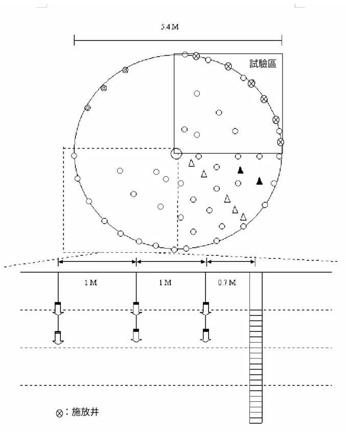
The field test for soil vapor extraction was conducted in the experimental farm of National Taiwan University in Hsin-tein. The SVE site had a radius of 2.7 meters and covered with 15-cm bentonite layer to avoid air leaking into the sucking well. Around the suction well there were 10 monitoring well in a quarter of a circle shown in Figure 2.2.

The diameter of the suction well was 6 inches. The screen opened between thedepth of 1 meter to 4 meter with total opening length of 3 meters. The monitoring wells were distributed in a quarter circle with depth around 1 meter to 1.8 meter depth which were installed by applying a direct push-in probe to drill a 2-inch hole, putting one or more Teflon tubes with screened aluminum heads at the desired positions then stuffing the surrounding of the head with quartz sands and sealing the hole with bentonite.

Samples were taken from the Teflon tubes with a hand pump. The suction wellwas connected to a demister and a vacuum pump at a suction head of 50 inches of water and a flow rate at 80 cfm. Sulfur hexafluoride, SF6, gas was used as the

tracer, which has little affinity with soils , no toxicity, high persistency in soils and high sensitivity for detection.

Before the tracer test was conducted the site had been condition for one day by suction at the previously described operational conditions. Fifty cubic centimeters of SF6 were injected in each of the six injection wells while the sucking pump was

temporarily stopped. Suction was started immediately after the tracer being injected. Samples were taken at different times and analyzed with GC-ECD for the gaseous

(23)

concentration of SF6.

The geology of the site is shown in Table 2.2.

The governing equation of the transport of a tracer in a cylindrical coordinate system is

( )

r C r C r r C D t C _g _g _g g g ∂ ∂ −         ∂ ∂ + ∂ ∂ = ∂ ∂ 1 ν 2 2 gm gf g D D D = + ν ξ⋅ = gm D H R Q v ⋅ ⋅ = ₂ π

ξ is the dispersivity (cm)，Q is the flow rate (cm3

/min)，H is the length of the

screen (cm)，R is the radius of the well (cm)， is the molecular diffusion

coefficient (cm

gf

D

2

/min). The only fitting parameters above is dispersivity. All other parameters can be measured on site. Q is 565.2 cm3/min, the length of the screen is 300 cm，molecular diffusion coefficient is 3.66 cm2/min。

Assuming that the injected tracer at 250 cm from the center is evenly distributed in a 2 cm by 300 cm layer of soils. The outer boundary was set at 300 cm from the center. The boundary conditions are

r = 300 cm 0 = g C 0 = ∂ ∂ r C_g r = 0 cm

The initial condition at t = 0 is

0

C

C_g = at r = 249 - 251 cm Cg =0 otherwise

(24)

Table 2.2 The geology of the SVE sits

Soil particle size distribution (%) depth

(m) description _gravel _{sand silt caly} Water content (%) Bulk density (g/cm3) 0~0.5 Grayish dark silt

with sands 0 47.5 44.2 8.3 17.7 1.41

0.5~1.5 Yellow brown

sandy soil 3.3 42.1 47.1 7.5 16.8 1.65

1.5~3

Yellow brown sandy soil with

gravels 3~4.5 Yellow brown

sandy soil

4.5~5.5 Grayish caly

2.3.5. Soil heterogeneity characterization

Traditional methods have been used to characterized the heterogeneity of the subsurface soil layer. Mechanical soil texture analysis of segments of a soil sample core will give the vertical distribution of the soil texture along the depth. Profile of the hydraulic conductivity of the soil layer is obtained by measuring the permeation of core segment by a permeameter. The soil moisture content also shows the porosity and heterogeneity of the soil column.

A new technique, Geo VIS, that can avoid the tedious sampling and analyses in the laboratory and uncover the profile the soil texture and some properties has been developed (Fig. 2.3). A frill rod is equipped with a video camera in side the belly and project to the surrounding soil stratum through a quartz window. Video signals are transmit to a monitor or a video recorder. The resolution of the camera is finer than 0.01 mm, which is fine enough to distinguish between clayey and sandy soils. Also, the equipment can be used to explore any NAPL in the aquifers. In this study, the technique was used to identify and locate the layers with high hydraulic conductivity and layers with low hydraulic conductivity, or say the heterogeneity of the soil column.

(25)

試驗區

：施放井

Figure 2.2 The locations of the suction well, injection wells and sampling wells on the SVE experimental site

(26)

Figure 2.3 The schematic diagram of the In-situ video geo-probe (Geo VIS)

2.4. Results and discussion

2.4.1. Column experimental results

We have been using the advection-diffusion governing equation to simulate the transport of tracer in soil column with the consideration of immediate equilibration between the mobile phases and immobile phases, or only first-order sorption kinetics, or two-stage first-order (two-box) sorption kinetics, or a distribution of mass-transfer limiting immobile regions. We found that the equilibration assumption or the first-order sorption kinetics approaches were not able to satisfactorily describe the experiment results.

(27)

Adopting a numerical approach we separate the distribution of the immobile regions into 10 groups. The jth group has a coefficient αsj and a fraction

(probability density) fsj., where

Σ fsj =1, j = 1 to 10

fs is a normal distribution density function in the respect of y, that is

fsj = fsj(yj) = F(yj+1/2) – F(y j-1/2), j=1 to 10

where F(z) = Pr(Z≦z) is a normal distribution function.

yj = log(αsj) ,

αsj=10Yi ,

yj+1/2 = yj + 0.5 ∆ y,

yj-1/2 = yj - 0.5 ∆ y

and ∆ y is the segment width. The distribution function has a mean µ and a standard deviation SD. Also

yj=μ+z*SD, -2.5 < z < 2.5

The breakthrough curve of soil column A shows slightly tailing and a retardation factor of 23.3, while soil column A shows significant tailing and much small

retardation factor of 3.4 (Fig. 2.4 and Fig. 2.5). Moisturizing the soil would greatly reduce the sorption capacity of the soil, facilitate the removal of the contaminant, however, likely to increase the heterogeneity of the porous matrix (with more significant tailing).

The best-fitting values of model parameters are shown in Table 2.3. The total fraction of the mobile phases.

(28)

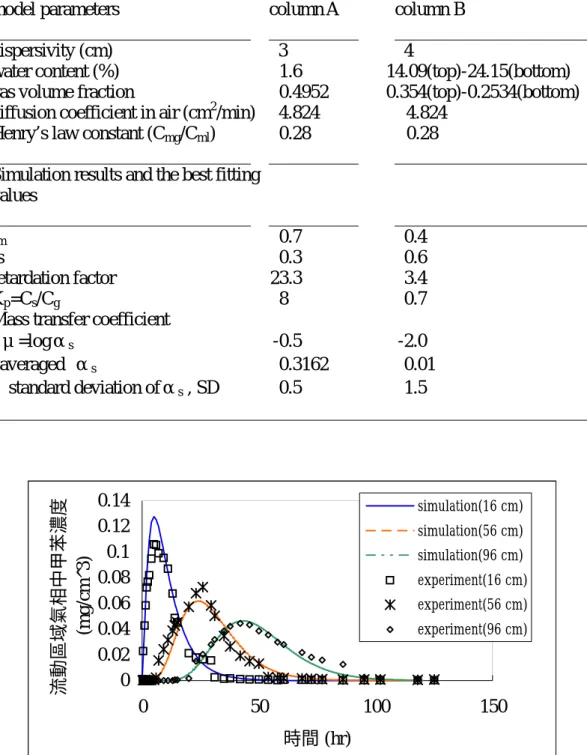
Table 2.3 The modeling parameters and the results of model simulation

___________________________________________________________________

model parameters column A column B

_____________________________ __________ ______________________

dispersivity (cm) 3 4

water content (%) 1.6 14.09(top)-24.15(bottom)

gas volume fraction 0.4952 0.354(top)-0.2534(bottom) diffusion coefficient in air (cm2/min) 4.824 4.824

Henry’s law constant (Cmg/Cml) 0.28 0.28

_____________________________ __________ ______________________ Simulation results and the best fitting

values _____________________________ __________ ______________________ fm 0.7 0.4 fs 0.3 0.6 retardation factor 23.3 3.4 Kp=Cs/Cg 8 0.7

Mass transfer coefficient

μ=logαs -0.5 -2.0

averaged αs 0.3162 0.01

standard deviation ofαs , SD 0.5 1.5

___________________________________________________________________ 0 0.02 0.04 0.06 0.08 0.1 0.12 0.14 0 50 100 150 時間 (hr) 流動區域氣相中甲苯濃度 (mg/cm^3) simulation(16 cm) simulation(56 cm) simulation(96 cm) experiment(16 cm) experiment(56 cm) experiment(96 cm)

Figure 2.4 The concentration of toluene at the locations of 16 cm, 56 cm, and 96 cm from the top of the soil column, respectively, in column A packed with dry soils (symbols) and the model simulation results (lines). A log-normal distribution of the mass-transferring coefficients is adopted with the mean at 0.32 and standard deviation at 0.5.

(29)

0 0.02 0.04 0.06 0.08 0.1 0.12 0.14 0.16 0 20 40 60 80

Time (hr)

Cgo (

m

g/ml)

5 cm 10 cm 20 cm 30 cm 5-fit 10-fit 20-fit 30-fit

Figure 2.5 The concentration of toluene at the locations of 5 cm, 10 cm, and 20 cm from the top of the soil column, respectively, in column B packed with water-soaked soils (symbols) and the model simulation results (lines). A log-normal distribution of the mass-transferring coefficients is adopted with the mean at 0.01 and standard deviation at 1.5.

The distributed mass-transfer coefficient approach is obviously able to simulate the transport of pollutants where there is heterogeneous soil texture and mass-transfer limited partition kinetics. The tailing of the breakthrough curve can be described quite well. Comparing the best-fitting parameters, we found that the mean of the mass-transfer coefficients of the moisturized soil column was much lower (by a factor of 30) than that of the dry soil column. It indicates that the transfer of the tracer between the mobile phases and the immobile phases in the moisturized is much slower. The reason of the slower equilibration is believably due the larger sizes of the immobile phases, which are the result of blockage of the gas channels by capillary water. Also, due to the uneven distribution of water in the soil column, the variation of the size of stagnant aggregates is high, which is reflected by the larger standard deviation of the fitting mass-transfer coefficient.

2.4.2. Tracer test on a soil-vapor-extraction field site

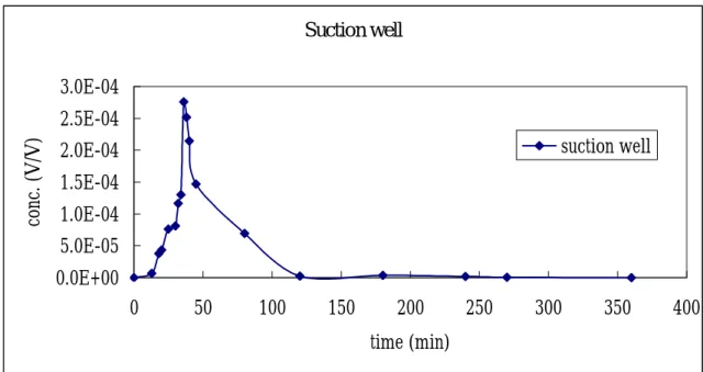
The concentrations of SF6 at the suction well, 70 cm from the well and 150 cm

from the well at different time are shown in Figure 2.6 to Figure 2.8. The peak of the concentration passed through the suction well 34 minutes after the beginning.

(30)

Suction well 0.0E+00 5.0E-05 1.0E-04 1.5E-04 2.0E-04 2.5E-04 3.0E-04 0 50 100 150 200 250 300 350 400 time (min) conc. (V/V) suction well

Figure2.6 The breakthrough curve of tracer at the suction well

r=70 cm 0.0E+00 1.0E-03 2.0E-03 3.0E-03 4.0E-03 5.0E-03 0 50 100 150 200 250 300 350 400 time (min) conc. (V/V) r=70cm

Figure 2.7 The breakthrough curve of tracer at the sampling well 70 cm from the center

(31)

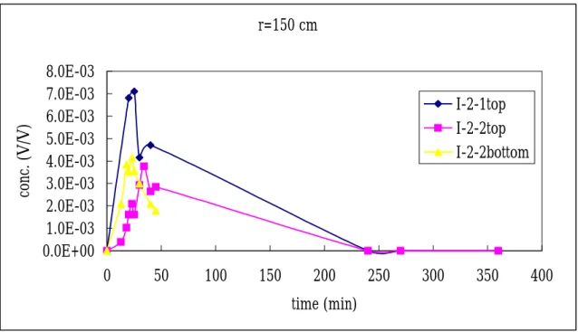
r=150 cm 0.0E+00 1.0E-03 2.0E-03 3.0E-03 4.0E-03 5.0E-03 6.0E-03 7.0E-03 8.0E-03 0 50 100 150 200 250 300 350 400 time (min) conc. (V/V) I-2-1top I-2-2top I-2-2bottom

Figure 2.8 The breakthrough curve of tracer at the sampling well 150 cm from the center

2.4.3. Application of soil video imaging system to in-situ soil monitoring

The soil video imaging system was fabricated that utilize a micro imaging device in internal part of a drill rod. The soil video imaging system is an on-line image monitoring system that can be applied to capture the continuous images of soil profile through a digital camera to perform the soil texture distribution investigation while drilling into the subsurface soil layer (see Fig. 2.9). Due to the limitation of budget, we were not able to apply any hydraulic pressurizing driller. Therefore, only images from shallow soil column were obtained (Fig. 2.10).

One snap shot is shown as Fig. 2.11 , the resolution of this photo is around 10 um, and the diameters of the observed soil aggregates were in the range of 10 um and 100 um. The continuously on-line images were converted to the mpeg files.

Apparently different soil texture distributions were observed from soil core samples at different depth. At a deeper location, the image indicates a finer and more uniform soil texture than that at the depth of 80 cm (Fig. 2.11). With a continuous image of the soil profile, we will be able to identify soil layers with relatively high permeability or layers with relatively low permeability.

(32)

Figure 2.9 Soil video imaging system. The drilling rod. Figure 2.10 The image of the texture of soil at depth of 80 cm.

Figure 2.11 The image of the texture of soil at a depth larger than 80 cm.

The results show that using this technique to distinguish between clayey and sandy soils. Also, the equipment can be used to identify and locate the layers with high hydraulic conductivity and layers with low hydraulic conductivity, or say the heterogeneity of the soil column.

2.5. Conclusions

The distributed mass-transfer coefficient approach is able to model the transport of pollutants where there is heterogeneous soil texture and mass-transfer limited partition kinetics. The experimental and simulation results also indicate that in a

(33)

length scale larger than that of a laboratory soil column the phenomenon of

non-equilibrium transport or tailing is resulted mainly from the mass-transfer limited migration of the sorbate into the stagnant region inside the immobile phases. The problem of modeling each of these immobile phases due to the lack of geological information can be improved by using a distributed mass-transfer coefficient set, which is related to some of the easily obtained soil properties such as the length scale of the system of concerned, the moisture content and the heterogeneity of the soil texture profile. Also the soil video imaging system can be used to identify and locate the layers with high hydraulic conductivity and layers with low hydraulic conductivity, or say the heterogeneity of the soil column with quite low cost and in short time, which will be a promising tool to help on the characterizing, modeling and remediation of a contaminated site.

(34)

Chapter 3 Sorption Kinetics of Toluene in Humin under Two

Different Levels of Relative Humidity

3.1 Introduction

The rate of sorption/desorption of volatile organic compounds (VOCs) plays an important role in pollutant fate modeling and contaminated soil remediation. Irreversible VOC sorption to or slow VOC desorption from soils in laboratory studies or field scales has been reported (Aochi and Farmer, 1995; Pingatello and Xing, 1996). It is found that a portion of VOCs desorbs very slowly from soil particles and a certain fraction of it is retained strongly by the particles (Steinberg et al., 1987; Pingatello, 1990). The retention of VOCs by soil components affects the fate of pollutants in the environment and the effectiveness of contaminated soil and aquifer remediation. Delineation of the sorption rate and of the reversibility of the sorption process with essential soil components is necessary to better predict the rates of pollutant migration and attenuation in soil.

Soil, a chemically heterogeneous matrix, contains various inorganic and organic components that each exhibits unique sorption behavior for pollutants (Chiou, 1998). The chemical heterogeneity complicates the prediction of the sorption or desorption rates of pollutants in the soil. Recent studies reveal the existence of a slow sorption/desorption of some organic compounds with soils (Luthy et al., 1997; Pignatello and Xing, 1996). This phenomenon has been attributed in part to a slow diffusion of the compounds through the micropores of soil particles (Farrell and Reinhard, 1994; Lin et al., 1994) and in part to their slow migration through soil organic matter (SOM) (Brusseau et al., 1991; Fu et al., 1994).

Sorption to humic substances is contended to contribute to the irreversible retention of xenobiotic compounds by soil (Cheshire, 1979). However, the sorption of toluene to humic acid, an integral member of soil humic substance, is found to be reversible and diffusion-controlled (Chang et al., 1997). Since humin represents a highly stable, recalcitrant, and high-molecular-weight fraction of SOM (Almendros et al., 1996; Hatcher et al., 1985), it may behave differently than the humic acid in the kinetics of sorption. Due to its cross-linked structure, humin may be capable of retaining VOCs for a significantly longer time and thus contribute to the slow or apparent irreversible sorption.

(35)

effect, due to the existence of a small amount of high-surface-area carbonaceous material (Chiou et al., 2000), the soil organic matter, including humin, behaves by and large like a partition medium for VOCs (Boyd et al., 1988; Chiou, 1988; Chiou et al., 1990; Chiou and Kile, 1994; Chiou, 1998). The amorphous humic structure provides a “solvent-like” medium that organic molecules can enter into or escape from it according to the thermodynamic gradient.

Humin is defined as the portion of humic materials that is insoluble in an aqueous solution at any pH. To be separated from the inorganic minerals in soils, humin is obtained by extensive digestion of soils with a mixture of concentrated HF and HCl (Stevenson, 1982). The HF/HCl extraction method has been widely applied for humin preparation (Chefetz et al., 2000; Grasset and Ambles, 1998; Guthrie et al., 1999; Lichtfouse et al., 1998a; Lichtfouse et al., 1998b), while the MIBK (methyl isobutyl ketone) method, as suggested by Rice and MacCarthy (1990), has also been applied for extraction of humin. In the MIBK method, humic substances are allowed to partition between water and MIBK as a function of the pH in water phase. Humin is then isolated from fulvic acid and humic acid. However, this method is so selective that some humin component could not be retrieved by MIBK. To meet the purpose of our experiment on the sorption/desorption rate of toluene with near natural humin, the solvent extraction was not adopted in order to prevent a significant alteration of the humic composition.

A spectroscopic approach has been adopted to address the interaction between VOCs and humic substances by Aochi and Farmer (1997). The authors investigated the sorption/desorption behavior of 1,2-dicholoethane on humic acid and fulvic acid under dry conditions. They found that an absorbance band increases continuously after days of desorption and the sorbed chemical was strongly retained. However, the sorption kinetics of VOCs on humin in a system resembling the natural level of humidity on a short time scale (say, minutes) has not been investigated. In this study, toluene, a model nonpolar, mononuclear hydrocarbon, was used as the sorbate to delineate the sorption behavior of VOCs with humin. Humin disks were prepared and used to study the rate of transport of toluene in humin matrix with artificially exaggerated mass transfer distance. Thin humin films were also used to mimic natural humin in a near-natural soil environment.

3.2 Materials and Methods

3.2.1 Soil Sample

Approximately ten kilograms of Yamingshan soil, classified as medial, thermic, Pachic Melanudands according to the definition by USDA (USDA-NRCS, 1993), were

(36)

air-dried, freed of large plant debris, and screened through a 20-mesh (0.84 mm) sieve. Small plant debris was further removed by flotation using ethanol. Then, soil sample was mixed well.

3.2.2 Humin

Humin was extracted according to the procedure developed by Rigol et al. (1998) and Russell et al. (1983) except that an ethanol/hexane mixture (1:1 v/v) was used to remove fats and waxes to avoid the interference from toluene, which is the target VOC to be studied. In short, soil was refluxed to remove fats and waxes and extracted by sodium hydroxide to remove humic acids and fulvic acids. The solid residue was separated by centrifugation, neutralized with 6 M HCl, washed with 0.1 M HCl and deionized water, and finally freeze-dried. The humin fraction was isolated from the solid residue by sequentially removing the mineral matter with a three-step digestion procedure: first, suspension in a 1:1 mixture of 0.2 M HF and 0.2 M HCl (20 ml/g) for 64 hours; subsequently, digestion in a 1:1 HF (5.5 M) and HCl (1.1 M) mixture for 1 hour three times; and, finally, digestion in 5.5 M HF four times for 16 hours each time. After centrifuging and washing with 0.1 M HCl and water three times, the final residue designated as humin was freeze-dried and ready for use.

A previous investigation by IR spectroscopy (Rigol et al., 1998) suggested that the treatment of soils with HF decreases the structural mineral matter content with relatively little influence on the nature of humin. Despite the challenges presented by modification, humin obtained by HF-extraction procedure were used for some sorption experiments (Chefetz et al., 2000; Gurthrie et al., 1999; Rigol et al., 1998). The

13_{C-NMR spectrum (not presented) of the solid residue after removal of waxes, humic}

and fulvic acids, and treatment by weak acids before severe HF/HCl extraction, is the same as that of the humin product after the severe HF/HCl treatment. The severe treatment procedure removed most of soil inorganic components while the humin components were preserved.

3.2.3 Sample Characterization

Element Analysis. Elements such as C, H, and N of humin were quantified in

triplicate samples using an Element Analyzer (EA) (Perkin-Elmer CHN-2400). Inorganic carbon was removed according to Ball et al. (1990). To determine the contents of major elements such as Fe, Al, Si, and Ca, samples were pretreated by fusion with LiBO2 at 1000oC for 30 min. The product was dissolved in 0.9 M HNO3

(37)

triplicates by inductively coupled plasma optical emission spectroscopy (ICP-OES) (Ingamells, 1970; Rigol et al., 1998).

Solid-State 13C-NMR Spectrometry. The cross polarization/magic angle spinning

(CP/MAS) 13C spectra of samples were measured on a Bruker DSX400WB NMR Spectrometer with a 7-mm diameter probe. The spinning rate was 7000 Hz. The acquisition parameters included contact time of 1 ms, pulse delay of 1 s, and pulse width of 4.2 µs.

The 13C-NMR spectra were analyzed according to the chemical-shift assignments made by Perminova et al. (1999) and Chefetz et al. (2000): 5-50 ppm, aliphatic H and C-substituted C atoms; 50-108 ppm, aliphatic O-substituted C atoms; 108-145 ppm, aromatic H and C-substituted C atoms; 145-163 ppm, aromatic O-substituted atoms; 163-190 ppm, C atoms of carboxylic, esteric, and amide groups. The distribution of C in each structural group was calculated as the percentage to the total carbon. The region between 5 to 108 ppm was calculated as aliphatic C and 108 to 163 ppm as aromatic C. The total aromaticity was calculated by expressing the aromatic C as a percentage of the sum of aliphatic and aromatic C; the total aliphaticity was calculated as the percentage of aliphatic C to the sum of aliphatic and aromatic C (Hatcher et al., 1981; Hatcher et al., 1983). The regions 50-108 ppm and 145-190 ppm were calculated as O- or N- substituted C atoms. The polarity was assigned based on the percentage of the sum of O- and N- substituted C atoms.

3.2.4 Preparation of Humin Disks

Humin disks were prepared by pressing the humin powder under a pressure of 12.7 N/m2 for 1.5 min (Chang et al., 1997). Four disks, all being 12.45 mm in diameter, were 0.34 mm, 0.44 mm, 0.61mm, and 0.64 mm in thickness, and weighed 61.5 mg, 72.8 mg, 100.2 mg, and 102.5 mg, respectively. Their bulk densities were 1.49 g/cm3, 1.36 g/cm3, 1.35 g/cm3, and 1.32 g/cm3, respectively. The disks were oven-dried (105 oC) overnight and stored in a desiccator before use.

The scanning electron microscopy (SEM) photographs were taken with a Hitachi S-800 SEM. Figure 3-1 shows the SEM photographs of one of the disks prepared by the above-mentioned procedure. The surface morphology (Fig. 3-1a) and the exposed inner surface of a broken edge with only a few pores and cracks display the homogeneity of the disk.

3.2.5 Sorption/Desorption Experiment

(38)

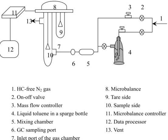
for sorption have been described elsewhere (Chang et al., 1997). Briefly, the experimental apparatus was maintained in a thermostatic room at 15±0.1oC, 25±0.1oC, or 35±0.1oC. The set temperature was closely monitored for at least one day to ensure its stability before initiation of the experiment. The disk was hung on the sample side of a Cahn 200 electric microbalance enclosed in a glass chamber. The toluene mass flux to the disk was significantly larger than the maximum toluene removal rate, which keeps the vapor concentrations inside the chamber at virtually fixed levels. The experiment was terminated when the change of weight could not be distinguished from the base noise of the microbalance, which was about 2 µg/5hr. The concentration of the toluene was determined with GC/FID (Hewlett-Packard 5890II).

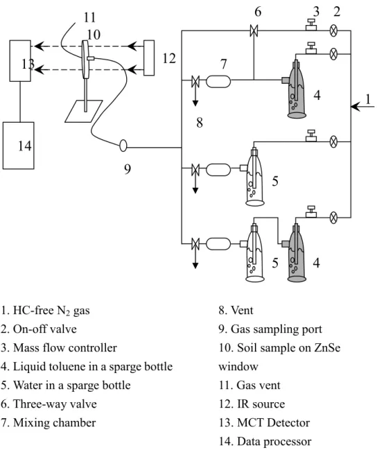
Sorption/Desorption Experiments Traced by FTIR. A drop of the humin

suspension in water was placed on the inner surface of a ZnSe window of a gas cell and dried in a desiccator. The absorbance spectra of IR beam passing through the gas cell windows were recorded on an IR spectrometer (BIO-Rad FTS 40) by averaging 200 scans at 2 cm-1 resolutions. The sample cell was purged with nitrogen gas carrying a constant toluene vapor concentration and relative humidity (RH below 1% for dry conditions and above 95% for humid conditions) during sorption experiments and purged with nitrogen gas without toluene during desorption experiments (Fig. 3-3).

3.2.6 Estimating Diffusivity

The diffusion model and its incorporation into the gravimetric method has been described in detail by Chang et al. (1997). The model development is briefly summarized here. The one-dimensional mass conservation equation is

2 2 x q D t q ∂ ∂ = ∂ ∂ (3-1) (3-2) dx t x q S t M l l

∫

− = ( , ) ) (

where q (mg/cm3) is the sorbate concentration in the disk at a distance x from the center plane of the disk and at time t; D is the apparent diffusivity of the sorbate inside the disk;

l is the half-thickness of the disk; M(t) is the total sorbed mass of sorbate in the disk; and S is the surface area of the disk.

Given the initial and boundary conditions,

(3-3) 0 ) 0 , (x = q (3-4) e q t l q(± ), =

(39)

0 ) , 0 ( = ∂ ∂ t x q (3-5)

The analytical solution for the fraction of equilibration is available in Crank and Park (Equations 36 and 37 in Chapter 1, 1968) and can be expressed as

) (t

f M

M_t _e = (3-6)

where Mt is the sorbed mass and f(t) is the dimensionless solution that is zero at t=0 and unity when t approaches infinity.

For the desorption process, the initial and boundary conditions are

(3-7) e q x q( ,0)= (3-8) 0 ) , (± tl = q

and Eq. 5. The analytical solution during desorption is )

( 1 f t M

M_t _e = − (3-9)

The diffusivity can be estimated by the best fit of the experimental results using the least-squares method.

3.3 Result and Discussion

3.3.1 Characteristics of Humin

The humin fraction contributes to 6.84% of the weight of the original soil and 15.9% of the weight of the total organic fraction (Table 3-1). The contents of the major elements, such as C, H, O, and N, in humin are shown in Table 3-2. The low atomic H/C ratio (1.08) indicates that a large fraction of the organic matter contains aromatic carbons. However, there is still a significant amount of aliphatic carbons according to the 13C-NMR results (Fig. 3-4).

Table 3-2 shows the amounts of Si, Al, and Fe in the humin fractions determined by ICP-OES. No noticeable amount of crystalline minerals can be detected through XRD (X-ray diffraction) observation. A small amount of these metals must be in amorphous form. The low inorganic content of the humin plus its low sorbing power for toluene did not significantly affect the sorption experiments.

The 13C-NMR spectrum of humin (Fig. 3-4) revealed the following composition: 50.2 % aliphatic moieties (32 ppm), 32.5 % carbohydrates (73 and 103 ppm), 14.4 % nonpolar aromatic compounds (128 ppm), and 2.9 % amide or carboxylic compounds (172 ppm) similar to the observation made by Chefetz et al. (2000). The total aromaticity of humin, 15.1 %, close to 8.8 % reported by Chefetz et al. (2000), is different from that of Aldrich humic acid (66.7 %) (Perminova et al., 1999). The major