台灣地區住宅存量與住宅價格之動態調整：失衡模型之應用

行政院國家科學委員會專題研究計畫 成果報告

台灣地區住宅存量與住宅價格之動態調整：失衡模型之應

用

研究成果報告(精簡版)

計 畫 類 別 ： 個別型

計 畫 編 號 ： NSC 95-2415-H-004-015-

執 行 期 間 ： 95 年 08 月 01 日至 96 年 07 月 31 日

執 行 單 位 ： 國立政治大學經濟學系

計 畫 主 持 人 ： 林祖嘉

計畫參與人員： 教授-主持人(含共同主持人)：林祖嘉

報 告 附 件 ： 國外研究心得報告

處 理 方 式 ： 本計畫可公開查詢

中 華 民 國 97 年 05 月 12 日

台灣地區住宅存量與住宅價格之動態調整：失衡模型之應用

*

林祖嘉

**

_{、馬毓駿**}

2008.5.

摘要

台灣住宅市場的的空屋率一直居高不下，自 1980 年初期的 7%水準攀升至

2007 年的 13%水準，期間經歷 1991 年的容積率管制措施，造成往後幾年的住宅

供給量大增。在此一情況下，再加上建物的耐久財特性，使得台灣房地產經歷了

長期的不景氣。然而，如果供需機制能有效運作時，理應能消化此一過多的餘屋，

然我們卻發現空屋率依舊維持在相對的高水位，顯示出台灣住宅市場呈現長期的

失衡現象。

本文嘗試由存量、流量的架構出發，建構一失衡調整模型，研究台灣在 1980

年至 2007 年間，住宅市場的價量動態調整過程，藉由此一機制，我們將可發現

台灣住宅市場價量變化的特性。然此一失衡模型之應用亦有極限，特別是未考量

政策因素與區域特徵將導致偏誤的估計值，本文亦提出進一步修正此一模型的可

能性。

關鍵詞：住宅存量、住宅價格、失衡模型

JEL Classification：R21, R31

* 本文為初稿，未經作者同意請勿引用。作者感謝國科會研究計畫（NSC95-2415-H-004-015）的 財務協助。 ** 兩位作者分別為政大經濟系教授與博士班研究生，聯絡方式，

一、前言

住宅市場中的需求行為與供給行為，一直都是住宅領域中重要的研究課題。

比方說，許多國內外學者估計住宅的需求彈性與所得彈性， 例如Hanushek and

Quigley(1990) 、Glennon(1989)、吳森田(1994)、吳森田與吳祥華(2004)、與林祖嘉

與 林 素 菁 (1994) 等 。 也 有 許 多 學 者 估 計 住 宅 供 給 彈 性 ， 例 如 de Leeuw and

Ekanem(1971)、Smith(1976)、與林素菁與林祖嘉(2001)等等。

也有不少學者同時考慮住宅市場的供需，以均衡模型來探討住宅市場的狀

況，例如Rosenand Smith(1983)、Wheaton(1990)、林祖嘉等(1994)、花敬群(2001)、

與彭建文(2004)等。這些研究除了探討住宅市場的供需行為以外，也同時探討空

屋率的問題。另外，也有一些文章直接研究住宅價格變動與存量調整的關係，例

如Heckman(1985)與花敬群與張金鶚(1997)。

上述的研究都是基於一個最基本的假設，即住宅市場是處於均衡的狀態，所

以可以利用傳統的均衡分析來處理。然而，住宅市場中有幾個特性，使得許多學

者對於住宅市場是否處於均衡狀態一直都有很大的爭議。第一，住宅的調整(或

遷徙)成本很高，使得有些家計單位雖然對於住宅需求已有改變(例如家庭人口增

加或減少)，但仍不願意調整其住宅消費，造成失衡。第二，由於住宅的異質性

很大，市場訊息又不充分，使得住宅需求雙方不易找到相合的適當交易對象，造

成住宅市場上經濟出現很大的價格分散(price dispersion)，例如林祖嘉(1994)。在

供需雙方都缺乏訊息下，很容易造成住宅市場的失衡。第三，由於住宅的興建速

度較慢，再加上供需雙方對於市場價格的反應與調整較慢，於是造成住宅市場的

失衡(disequilibrium)，而且往均衡調整的速度很慢，可參見Fair(1972)、DiPasquale

and Wheaton (1994)、與Riddle(2004)。由於住宅市場缺乏訊息的結果，也造成住宅

市場缺乏效率性，見Case and Shiller(1989)。

以國內的住宅市場來看，過去三次人口普查(1980、1990、與2000)，台灣住

宅的空屋率分別高達(12.65%、13.16%、與18.19%)。雖然林祖嘉等(1994)與彭建文

(2004)等研究指出台灣的均衡空屋率很高，我們仍然無法否認台灣市場上的兩大

特性，即住宅市場的長期失衡是存在的，同時，住宅市場往均衡調整的速度很慢，

這兩個現象與國外學者研究國外市場得到的結果十分相似。

既然國內的住宅市場具有長期失衡的現象，我們仍使用均衡模型來討論住宅

供需，在方法上是否適當？或許我們應該改用失衡模型來處理台灣住宅市場的供

需較為妥當？這個問題不但在學術上很重要，而且也具有很重要的政策意義。因

為如果失衡模型較好，那麼過去對於住宅市場供需的估計可能都會有問題，或者

至少會產生一些偏誤。而不幸得是，雖然我們看到台灣住宅市場長期處於失衡狀

態，但國內文獻卻一直缺乏採用失衡模型來處理市場供需與市場調整的問題。

所採用的失衡模型，來探討國內住宅市場的狀況。本文先建立一個簡單的失衡供

需模型，然後加入部分調整模型，再將之轉換成計量模型，最後再以台灣地區

1982 到 2007 年住宅市場 26 年的季資料來測試住宅市場的供需與調整速度。由於

國內採用失衡模型的研究很少，在住宅市場上更可能是第一次嘗試，所以本文對

於國內研究住宅領域方面應該有很重要的學術價值。

二、失衡模型

(1) 失衡模型的建立

依據 Fair(1972)與 Fair and Jaffee(1972)的失衡模型，第 t 年住宅市場的需求曲線

(

HD

_t

)與供給曲線(

HS

_t

)分別可以寫成

e t t t HD =HD +u

(1)

e t t t HS =HS +v

(2)

其中

u

_t

與 代表影響需求與供給的誤差項(不均衡量)，

v

_t e t HD

與

HSte

分別代表長期

均衡的需求與供給，其分別決定於相關的解釋變數，可分別寫成

0 1 e t t t HD =

α

+

α

P+ XD t

(3)

0 1 e t t HS =

β

+

β

P+ XS

(4)

其中

P

_t

為市場價格；

XD 與

_t

XS 則是決定長期住宅需求與供給的有關變數，

_t

本研究稍後有更詳細的說明。

再依失衡理論，第 t 年的實際交易量(

HD

_t

)(或是可看成長期均衡量

e t HD

)決定

於需求量(

HD

_t

)與供給量(

HS

_t

)較小的一方，即

min(

,

)

t t

HQ

=

HD HS

_t

(5)

或是

, , t t t t t

HD

if HD

HS

HQ

HS

if HS

HD

≤

⎧

= ⎨

_≤

⎩

t t t t t

(6)

或是

(1

)

t t

HQ

=

kHD

+ −

k HS

(7)

其中

, , , ,

0

1

t t t t t t

if HQ

HD or HD

HS

k

if HQ

HS or HS

HD

=

≤

⎧

= ⎨

₌

_≤

⎩

在住宅市場上，由於住宅是一種標準的耐久財(durable goods)，在市場不均衡

的情況下，每期數量的變化會決定於本期均衡交易量

e t HQ

與前期存量

的差

異。依 DiPasquale and Wheaton(1994)與 Riddle(2004)，此一住宅存量調整(

)可用

部分調整模型(partial adjustment model)來處理，即

1 t

HQ

₋ t

S

Δ

1 ( e ) t t S

γ

HQ HQ₋ Δ = − _t )

(8)

同樣的，住宅價格的調整也決定於本期均價格(

e

)與前期價格的差異，即

t P 1 ( e t t t P

δ

P P₋ Δ = −

(9)

其中

γ 代表住宅數量的調整速度，

δ

則代表住宅價格的調整速度。由於住宅

興建大約需要兩年以上的時間，再加上通常每年住宅興建的數量(即住宅投資)大

約只有住宅存量的 2%到 3%左右，所以理論上來說，短期下住宅數量往均衡調整

的速度較慢，而長期下才可能看到較大的調整。反之，住宅價格則可以有較快的

調整，所以一般而言，

γ 要小於

δ

。

(2)失衡模型的估計

在估計失衡模型方面，通常會有二個步驟，第一個步驟是先估計住宅的需求

函數與住宅的供給函數，即上述的(1)與(2)式。然後，我們再把(1)式及(2)式代入

(8)式與(9)式當中，可以得到(8)式與(9)式的縮減式(reduced form)。依 Riddle(2004)，

此縮減式可寫成：

0 1 2 3 4 1 5 1 t t t t t t

S

a

a P

a

XD

a

XS

a u

₋

a v

₋

ε

_t

Δ =

+ Δ + Δ

+ Δ

+

+

+ (10)

0 1 2 3 4 1 5 1 t t t t t t

P

b

b S

b XD

b XS

b u

₋

b v

₋

e

Δ = + Δ + Δ

+ Δ

+

+

+

_t

(11)

其中

Δ

XD

_t

是關於影響住宅需求相關變數的變動量，

Δ

XS

_t

是關於影響住宅

供給相關變數的變動量，

u

_t−1

與

v

_t−1

則是前一期需求變數與供給函數的差額(即不

均衡下的數額)，此

u

_t−1

與

v

_t−1

的估計可由(1)式與(2)式的估計式中得到。而

ε

_t

與 則

符合傳統誤差項的假設。

t

e

就住宅市場失衡模型而言，我們最在意的是前期失衡量(

u

_t−1

與

)對於本期

數量變化(

)與價格變化(

)的影響，亦即

a 、

₄

a

₅

b

₄

b 的符號方向與大

₅

小。就理論上來看，當前期的住宅需求量(

u

_{t 1} 1 t

v

₋ t

S

Δ

Δ

P

_t

、

與

−

)太大(代表的是使需求曲線右移)，

或是前期供給量(

v

_t−1

)太大(代表的是使供給曲線右移)，都會引起本期存量(

Δ )

S

_t

的增

(即

a 、

₄

a 為正)。但另一方面，當前期住宅需求的失衡量(

₅

u

_t−1

)太大(代表

的是使需求曲線右移)，則會使本期價格(

P

_t

加

Δ )上升；而當前期住宅供給失衡量(

v

_t−1

)

太大(代表的是使供給曲線右移)，則會使本期價格

(

Δ )下降。換言之，我們預期

P

_t

、

。因此我們要檢定的假設有兩組，即在住宅數量調整方面，我們

要檢定的假設是：

4

0

b

>

b

₅

<

0

0 4 5 1 0

:

0,

:

H

a

a

H

not H

>

> 0

0

(12)

在住宅價格調整方面，我們要檢定的假設是：

0 4 5 1 0

:

0,

:

H

b

b

H

not H

>

<

(13)

最後，在計量分析架構方面，依一般時間數列分析的流程，我們首先進行數

列的定態檢定。理論上，因長短期的關係即為 DiPasquale and Wheaton(1994)與

Riddle(2004)所提及的存量-流量關係，而存量又為流量之累積，存量經一階差分

後即為流量分析，也就是式(10)與式(11)的失衡模型，故判定變數差分前後的階

次，是確保分析可靠性的首要條件。

在確定數列的階次後，遂進入式(3)與式(4)的長期均衡關係估計，本文在此

一階段將採用共整合估計的方式來描述變數間的關係。Riddle(2004)的研究則是在

確認變數階次後，直接以 OLS 估計其長期均衡關係，此一作法相對較不嚴謹，

稍後本研究有更詳細探討。在獲得長期關係之後，我們進一步計算此一方程式的

殘差值作為長期關係失衡時的代表，並以延遲一期的方式(

u

_t−1

與

v

_t−1

)呈現在式(10)

三、實證結果分析

(1) 資料來源與數列恆定檢定

依實證分析的需求，本文採用的變數相對較多，同時部分變數依研究需求亦

將略微修正，或資料長度不足而改以插補法的方式補足所需之觀察值。本研究期

間由 1982Q2 自 2007Q4，為季資料，共 103 季。在存量-流量的架構中，如DiPasquale

and Wheaton(1994)與Riddle(2004)的模型，採用住宅存量作為存量變數。而台灣住

宅存量登記始自 1990 年開始，時間長度過短且相對不精確，因此本文改以使用

執照面積(SQF)之累積量(CSQF)作為本文的存量變數。

1

在房價變數選取方面，因

國泰房價指數與信義房價指數時間長度過短而無法使用，本文以預售屋住宅價格

(HP)作為本文的住宅價格變數。在其餘的需求變數方面，本文亦將選取累積之家

戶數存量(HH)作為人口特徵變數，租金指數(RENT)作為租賃選擇變數，國民可支

配所得代表所得效果，再依Almon(1962)的方法，將國民可支配所得轉換成恆常

所得(PY)。

2

在衡量家戶需求的資金成本方面，本文以Dougherty and Van Order(1982)

定義的使用者成本(USERC)作為家戶借貸時的資金成本。

3

在影響供給量的選取方面，除累積執照面積(CSQF)外，本文採用的變數尚有

營建成本指數(CC)、空屋率(VAC)、GDP與代表建商短期融資成本的 90 天期商業

本票利率(TBR)。

4

因使用的變數頗多，為節省文章的篇幅與撰寫之流暢性，本文

一併於附錄中說明的資料定義與來源出處。此外，為方便實證結果的說明，除使

用者成本、商業本票利率與空屋率外，其餘變數均進行對數化處理，並以L加註

之。

在表一中，我們列出各主要變數的基本統計量，包括平均數與標準差。不過

由於我們使用的是時間數列分析，所以平均數只能當作一個很基本的參考資料，

而各主要變數時間數列的統計性質才是我們所關心的。

1 以衡量供給量變動的角度而言，因每件推案的面積均不相同，住宅存量記錄的方式相對較不精 確且容易失真。相對而言，使用執照面積則是代表當期實際產生的供給量，並以面積(平方公尺) 的方式紀錄，較易掌握建商真實的供給行為。 2 因家戶購買住宅必須考量長期的支付能力，以當期可支配所得描述可能略嫌不足，故研究以改 以恆常所得的概念定義所得需求變化的影響，Almon (1962)多項式時間落後模型( polynomial distributed lag)的定義為 0 ( ) [2 /( 1)] n ( ) n t i t i A Y = n+

∑

₌ n i Y− ₋，i=1…n，本文以n=4 計算恆常所得。 3 1 1

(

)(1

) 0.5(

/

) 0.5(

/

)

t t p y t t t t

USERC

=

i

+

t

−

t

−

Δ

HP HP

−

Δ

HP

₋

HP

₋ ， 與 分別代表地價 稅率與所得稅率，台灣的地價稅率極小(約千分之二)可忽略，所得稅率則以 33%表示， 為預

售屋住宅價格指數。Dougherty and Van Order(1982)站在已擁屋者的角度來看，當房價升值時，機 會成本較小。 p

t

t

_y t

HP

4 Riddel(2004)是以 90 天期的國庫券利率作為建商的短期資金成本，但台灣的國庫券交易並不似 美國熱絡，利率的變化相對較小，因此本文以商業本票利率來替代。

表一 變數基本統計量

變數

平均數

標準差

家戶數 (HH) (戶)

5775069 1043912

累積使用執照面積 (SQF) (平方公尺)

4.36E+08 2.77E+08

恆常所得水準 (PY) (百萬元)

6607104 2574400

國內生產毛額 (GDP) (百萬元)

1739177 860400

預售屋住宅價格 (HP) (萬)

13.501 5.370

租金指數 (RENT) (指數)

84.015 16.622

建築成本指數 (CC) (指數)

77.657 10.612

90 天期商業本票利率 (TBR) (%)

0.057 0.030

空屋率 (VAC) (%)

0.106 0.025

使用者成本 (USERC) (%)

0.040 0.053

資料來源：本研究。

表二 單根檢定結果

ADF 檢定統計量

變數

原始值

一次差分

家戶數 (HH)

-1.919

-3.352***

累積使用執照面積 (SQF)

1.247

-2.008**

恆常所得水準 (PY)

-0.809

-3.764**

預售屋住宅價格 (HP)

-2.105

-4.840***

國內生產毛額 (GDP)

-0.372

-4.506***

租金指數 (RENT)

0.729

-1.866*

建築成本指數 (CC)

0.653

-5.292***

90 天期商業本票利率 TBR

-3.004

-10.95***

空屋率 (VAC)

-1.061

-3.090**

使用者成本 (USERC)

-2.856

-11.697***

資料來源：本研究。

附 註：(a)表中數值代表檢定統計量。

(b)*、**與***分別代表在10%、5%與1%的顯著水準下拒絕數列為單

根的虛無假設。

在檢定數列是否為恆定數列上，本研究採用 ADF(Augmented Dickey-Fuller)的

檢定方法進行，並表列原始值與一次差分後的檢定結果。由表二的結果發現，本

文採用變數的原始數列皆顯著為非恆定數列，但再經一次差分後，所有數列均在

至少 10%的顯著水準下，均已呈現恆定狀態。經恆定狀態的檢定後，便可進入存

量-流量分析的架構。

(2) 實證結果

在前述理論說明中，本文已對將採用之架構有詳細的描述，同時在確定文中

使用數列的階次後，便可估計供需的長期需求關係，此部分也就是存量分析。接

著將所得之長期關係的殘差帶入短期關係中，也就是流量分析。本文首先就建構

供給與需求的長期均衡式工具說明。

以需求面而言，本文採用恆常所得、租金指數、使用者成本、家戶數與新成

屋房價作為影響需求的主要來源。同時本文依據 DiPasquale and Wheaton(1994)與

Riddle(2004)的作法，將需求函數定義在家戶數變化比例下的實質家戶需求，如下

所示：

(

,

)

t t t t

LCSQF

=

HH

⋅

f LP XD

+

u

_t

其中

XD 表示恆常所得、租金指數與使用者成本的水準值，亦即影響存量累

_t

積的因素是以家戶數的水準值加成(proportional)而來。同時為方便實際估計時的

運算，通常會將之改寫成：

( , ) t t t t LCSQF t t LPCSQF f LP XD u HH = = +

)

式中的 (

f LP XD 以本文而言為一線性關係，同時本文對殘差值

_t

,

_t

採用相同

的符號，因這並不影響我們的分析。

t

u

5

在供給面的長期關係方面，依舊由累積使

用執照面積表示供給存量，影響供給存量的來源，仍假定先前介紹過的變數，其

關係亦為線性。

在估計長期關係的工具方面，Riddle(2004)採用Engle and Granger的方法來決

定長期關係，此法相對而言有較多的缺點。

6

本文採用Johansen(1990)的方法來檢

定變數間是否存在共整合，此一共整合關係即為本文描述的需求(供給)的長期均

5 本文的作法是將累計使用執照面積發放的原始值除以家戶累計數後，在進行對數化處理，並以 P表示加成(proportional)之意。同時，本文亦對 進行單根檢定，發現原始值亦呈現單根 性質，經一次差分後，而在 5%的顯著水準下，已顯著拒絕單根的虛無假設。

LPCSQF

6

衡關係。Johansen(1990)的檢定結果如表三所示：

表三 共整合檢定

Hypothesized

No. of CE(s)

Trace test

Max test

None 136.887** 56.941**

需求面

At most 1 79.947** 51.575** None 195.316** 88.217**

供給面

At most 1 107.099** 42.911**

資料來源：本研究。

附 註：**與*分別表 5%與 10%的顯著水準下拒絕虛無假設。

Johansen 的共整合結果顯示，不論是需求的均衡式或供給的均衡式均存在不

止一條的長期關係式。理論上，實證研究者希望得到唯一的一條關係式，但事實

上，估計的過程不易獲得僅一條的關係式，特別是模型採用的變數為數較多時。

通常會採一較折衷的方式，即採用眾多關係式中，估計係數較符合經濟意義的關

係式作為說明，本文亦採此一作法。需求與供給的長期關係表示如下：

t t t t (0.136) (0.285) (1.022) (0.087)

LPCSQF

=

0.388*LPY + 2.820*LRENT -3.449*USERC - 0.510*LHP

_t

t

t t t t t (0.032) (0.058) (0.341) (0.063) (0.452)

LCSQF

=

0.216*LHP + 0.810*LGDP - 2.805*TBR - 0.046*LCC +1.356*VAC

上兩式中括弧內是 S.D.。其中長期需求關係式的參數估計結果均符合我們事

前的預期，而且係數顯著，恆常所得增加(0.388)會使住宅需求增加，租金增加

(2.820)會使租賃成本增加而衍生住宅需求。使用者成本(-3.449)的影響亦在預料之

中，當資金的機會成本越低，住宅的需求就越大。而當房價(-0.510)越低，住宅需

求相對較高亦是吾人所預期。

在供給方面，大多數的變數對供給量影響的亦如預期，房價越高時建商的供

給意願更大。DiPasquale and Wheaton(1994)認為住宅供給與GDP有一定比例關係，

GDP越高則供給量越大，本文得到的估計係數(0.810)亦支持此一論述。代表建商

短期融資成本的商業本票利率亦對供給量有顯著影響(-2.805)，利率越低則建商的

機會成本亦相對較小。建築成本的影響則未如我們預期的具有顯著影響，本文猜

測因建築成本指數的建構僅包含建築材料或人力成本，但卻未納入土地成本所

致。

7

最後，我們發現空屋率對供給的影響並未如本文預期(1.356)，正向且顯著的

影響顯然與理論不符，吾人造成此一結果可能來自於忽略區域差異所致。

在獲得長期均衡關係式後，我們計算二者共整合估計下長期關係式，並將之

以延遲一期的效果帶入價量的短期結構式中。在短期的價量調整式中，依據式(10)

與式(11)所述，將影響需求與供給均衡的外生變數，經一次差分後以延遲一期的

效果帶入短期調整式中。本文為防止可能遺漏變數延遲效果可能性，故將遲落效

果由 1 期延長至 3 期，並將估計過程中不顯著的估計係數予以剔除，僅保留 10%

以上的顯著水準下的估計係數值，並以此說明經濟意涵，估計係數彙整如表三所

示。

在表四的估計結果中，本文關注的是誤差修正估計係數

u

_t−1

與

，與本研究

事先的預期有所差距，住宅流量調整方程式對需求失衡的調整速度為-0.063，但

並不顯著。而當面對供給失衡時時，供給行為將持續擴大失衡狀態，以每期約

0.45 的速度增加，且此一效果具有統計上的顯著性，此一結論顯與吾人的猜測不

符，吾人對此結果的看法，將於說明價格調整方程式後一併分析。在價格調整方

程式方面，需求與供給的失衡都顯著的衝擊價格調整，誤差修正係數分別為-0.317

與 0.343，且都在 1%的顯著水準之上，面對需求的下降致使當期整體住宅價格下

降，相對符合經濟直覺與相關研究的結論。但面對供給失衡時，正向的誤差調整

係數說明當市場存在超額供給，將進一步推升房地產房價，此一結果亦與經濟直

覺相違背，且與流量調整方程式的結論雷同。

1 t

v

₋

吾人猜測造成此一估計的原因如下，第一，理論上，當市場存在超額供給時，

房價即使不會立即反應過多的供給，亦不至造成房價上漲。但若考慮台灣住宅市

場結構，確有可能促使此一情況發生，台灣建築業的景氣循環具有擴張期間短，

收縮期間長的特性，且擴張期間價格上漲迅速，當處於衰退期間，住宅價格的下

跌十分緩慢，甚至不明顯。輔以政府時常採用的購屋優惠貸款措施，更進一步阻

絕房價下跌的空間，此外，此一政策效果亦可能造成建商的預期心理，在餘屋過

多的情況下持續推案，遂使供給不減反增。

再者，政府於 1992 年實行建壁率與融資率管制措施，造成建商一窩蜂的搶

建風潮，遂造成往後數年的住宅供給量遽增，其餘總體特徵變數的變化卻相對平

穩。很明顯的，此一期間的供給行為明顯偏離長期均衡水準，而供給量與存量為

本文採用的應變數之一，在無其餘替代變數的情況下，此一政策影響的結果自然

會造成估計時的精確度下降，甚至是錯誤的結論。第三，忽略區域因素造成的差

異，區位特徵在住宅市場的扮演的地位不下於總體特徵變數，以台灣為例，台北

市是相對發展較早、也較快的區域，多數的土地都已開發，而以外的都會區發展

較晚且多屬平原地形，在此一先天結構下，土地取得的難易不同，造成價量調整

的過程不盡相同。忽略區域因素，亦可能是造成存量均衡式中，有關空屋率的估

計係數與理論不符的因素。

地成本的比重相對較高。

表四 住宅流量與房價部分調整方程式

住宅流量調整方程式

房價調整方程式

變數

估計係數

標準差

變數

估計係數

標準差

Constant 11.496

2.021

Constant -6.825 1.038

1 t

u

₋

-0.063 0.093

u

t−1

-0.317 0.048

1 t

v

₋

0.450 0.111

v

t−1

0.343 0.053

2 t

LPY

₋

Δ

-13.807

2.488

Δ

USERC

t

-1.442 0.118

1 t

LGDP

₋

Δ

11.326 2.585

Δ

USERC

t−1

0.392 0.124

2 t

LGDP

₋

Δ

4.422 1.423

Δ

USERC

t−2

-0.315 0.132

t

VAC

Δ

0.404

0.062

Δ

LRENT

t

8.897 1.162

2 t

VAC

₋

Δ

0.422 0.060

Δ

TBR

t

0.802 0.336

t

TBR

Δ

2.454 1.503

Δ

TBR

t−1

0.794 0.365

R-squared 0.678 R-squared

0.707

資料來源：本研究。

在短期特徵變化的影響方面，當期流量的調整明顯受實質所得的影響較大，

兩期的遲落效果皆為正向(11.326 與 4.422)。而遲落二期的房價變化影響為負

(-13.807)，表示房價越高則供給量越少，此一估計結果亦與實際觀察不符，推測

此一原因與遺漏重要變數或遲落效果超過兩期以上有關。空屋率的影響一如存量

均衡式一般，對當期供給量有正向影響(0.404 與 0.422)，與理論論述有不同的結

果，吾人對此一結果的解讀亦與為進行區位劃分有關。商業本票利率變化的影響

為正(2.454)，融資成本上升卻推升當期供給量，此結果亦可能是不同延遲效果所

致。

在房價調整方程式方面，使用者成本的變化顯然是構成房價變化的主因，不

同延遲期數有不同的效果(-1.442、0.392 與-0.315)，加總效果約為-1.4，說明當

使用者成本下降，其效果具有持續性之外，對房價的推升相對顯著。租金指數的

改變亦如本文的預期，對房價產生正向的間接效果(8.897)，當期租金越高的產

生的替代效果，致使住宅需求越高，進而推升房價。商業本票利率變化亦對房屋

價格變化有正向顯著的影響(0.802 與 0.794)，此一結果係透過供給面的管道傳遞，

本文亦傾向解釋為忽略區域因素所致。

四、結論

本文由存量-流量的架構出發，利用失衡模型來探討供給與需求的均衡關係

破壞時，如何衝擊短期價量的變化，以此來解讀台灣 20 餘年房地產市場，構成

價與量的主要因素。我們發現，以長期關係而言，以家戶變化為比例的住宅需求

與房價、恆常所得、租金水準與使用者成本構成一穩定的均衡關係。在供給方面，

亦發現存量與房價、GDP、90 天期商業本票利率與空屋率有顯著關連性，唯空屋

率的影響並產生預期的效果，本文推測可能是忽略區域因素所致。

在流量變化與房價的短期調整方面，需求面失衡僅對房價產生衝擊，未對流

量有顯著影響。而供給面的失衡雖顯著影響房價變化與住宅供給量的調整，但其

方向卻非吾人所預期，我們推測可能是來自於未考量政策效果或區域特徵所致。

此一效果亦影響部分外生變數短期間的變化對房價與供給量的衝擊，產生不符合

經濟直覺的估計係數。未來可進一步依區位劃分估計方程式，並尋找衡量政策效

果的可靠變數，將能使價量變化的失衡模型更精確的描述台灣房地產市場。

參考文獻

吳森田(1994)，“所得、貨幣與房價-近二十年台北地區的觀察＂，

住宅學報

，2，

25-48。

吳森田、吳祥華(2004)，“Affordability, Speculation and House Price in Taipei

＂，

住宅學報

，13(2)，1-22。

林祖嘉(1994)，“價格分散與搜尋均衡在台灣地區住宅市場之驗證＂，

經濟論文

叢刊

，22(2)，237-269。

林祖嘉、林素菁(1994)，“台灣地區住宅需求價格彈性與所得彈性之估計＂，

住

宅學報

，2，25-48。

林祖嘉、張金鶚、彭建文(1994)，“台灣地區空屋率與房價調整之均衡分析＂，

國科會八十二年度經濟學門專題計畫研究成果發表會論文集

，85-106。

林素菁、林祖嘉(2001)，“台灣地區住宅供給彈性之估計＂，

住宅學報

，10(1)，

17-27。

花敬群(2001)，“自有率、空屋數量與住宅市場調整＂，

住宅學報

，10(2)，

127-137。

花敬群、張金鶚(1997)，“住宅市場價量波動之研究＂，

住宅學報

，5，1-15。

彭建文(2004)，“台灣空屋狀況變遷與原因分析＂，

住宅學報

，2，23-46。

謝文盛(2001)，“再論土地增值稅與住宅價格之關係＂，

住宅學報

，10(2)，91-105。

Case, K.E., and R.J. Schiller (1989), “The Efficiency of the Market for Single

Family Homes,” American Economics Review, 79, 125-137.

Clapp, J.M., and C. Giaccotto (1994), “The Influence of Economic Variables on

Local House Price Dynamics,” Journal of Urban Economics, 36, 161-183.

de Leeuw, F., and N.F. Ekanem, (1971), “The Supply of Rental Housing,”

American Economics Review, 61(5), 806-817.

DiPasquale, D., and W. Wheaton (1994), “Housing Market Dynamics and the

Future of Housing Prices,” Journal of Urban Economics, 35, 1-27.

Dougherty, A., and R. Van Order (1982), “Inflation, Housing Costs and the

Consumer Price Index,” American Economic Review, 72(1), 154-164.

Fair R.C. (1972), “Disequilibrium in Housing Models,” Journal of Finance, 27(2),

207-221.

Fair, R.C., and D.M. Jaffee (1972), “Methods of Estimator for Markets in

Disequilibrium,” Econometrics, 40(3), 497-514.

Gabriel, S.A., and F.E. Nothaft (2001), “Rental Housing Markets, the Incidence

and Duration of Vacancy and the Natural Vacancy Rate,” Journal of the

American Real Estate and Urban Economics, 49(1),121-149.

Glennon, G.D. (1989), “Estimating the Income, Price, and Interest Elasticities

of Housing Demand,” Journal of Urban Economics, 25, 219-229.

Hanushek, E.A., and J.M.Quigley, (1980), “What is the Price Elasticity of

Housing Demand,” Review of Economics and Statistics, 62, 449-454.

Heckman, J.S.(1985), “Rental Price Adjustment and Investment in the Office

Market,” Journal of the American Real Estate and Urban Economics, 13,

32-47.

Mankiw, N.G., and D.N. Weil (1989), “The Baby Boom, the Baby Bust, and the

Housing Market,” Journal of Regional Science and Urban Economics, 19,

235-256.

Phillips, P.C., and M. Loretan (1991), “Estimating Long Run Economic

Equilibria,” Review of Economic Studies, 58, 407-436.

Riddel, M. (2004), ”Housing-Market Disequilibrium: an Examination of Housing

Market Price and Stock Dynamics,” Journal of Housing Economics, 13,

120-135.

Rosen, T., and B. Smith (1983), “The Price-Adjustment Process for Rental

Housing and Natural Vacancy Rate,” American Economic Review, 73(4),

779-786.

Smith, B.A. (1976), “The Supply of Urban Housing,” Quarterly Journal of

Economics, 90(3), 389-405.

Wheaton, W.C., (1990), “Vacancy, Search, and Prices in a Housing Market

Matching Model,” Journal of Political Economy, 98(6), 1270-1292.

附錄：資料來源說明

使用執照面積(SQF)(平方公尺)：內政部營建署。

預售屋住宅價格(HP)(萬元)：內政部營建署。

家戶數存量(HH)(戶)：中華民國人口統計月報。

租金指數(RENT)(指數)：內政部營建署。

恆常所得(PY)(Almon 定義轉換)：行政院主計處公布之國民可支配所得(單位為百

萬台幣)，本文以 Almon(1962)建議轉換成恆常所得定義。

國內生產毛額(GDP)(百萬)：行政院主計處發行之國民所得統計摘要。

使用者成本(USERC)(%)：金融統計月報之本國一般銀行放款利率，再依定義轉換

成使用者成本。

營建成本指數(CC)(指數)：資料來源為內政部營建署，原始資料自 1991 年開始以

月資料型態登錄，本文以算數平均將之轉換成季資料型態，並利用 AR(3)的模型

將插補至本文研究期間的起始點(1982Q1)。

空屋率(VAC)(%)：內政部營建署。利用台電紀錄之不足用電底數的家戶數資料。

90 天期商業本票利率(TBR)：金融統計月報。

國立政治大學補助學術活動執行成果報告書

填表日期：96 年 8 月 19 日

活動類別

□研究團隊 □學術研討會 Ⅴ 出席國際會議發表論文

□讀書會 □鼓勵教師及研究人員申請國科會專題研究計畫

□其他

申請人姓名 林祖嘉

服務單位 政大經濟系

職稱

Ⅴ 教師/研究人員

□博士生 □碩士生

電 話 29387462

e-mail [email protected]

實際活動起迄日期 2007.7.9 – 12

活動地點 澳門

活動名稱

（中文）第十三屆亞洲不動產學會與美國不動產與都市經濟學會

聯合年會

（英文）The 12

th

AsRES Annual Conference & The 2007 AREUEA

International Conference

National Chengchi University Faculty Attendance at International

Conferences--Report

19/80/2007 (dd/mm/yyyy)

Name

Chu –Chia Lin

Administrative Unit

and Job Title

Department of Economics

Professor

Location of

Conference

Macau

Duration of

Conference

09~12/07/2007

Name of Conference

(Chinese)

第十三屆亞洲不動產學會與美國不動產與都市經濟學會

聯合年會

(English)

The 12

th

AsRES Annual Conference & The 2007 AREUEA

International Conference

Title of Presented

Manuscript

Chinese)住宅環境與兒童教育表現關係的新證據：台灣的個案分析

(English) New Evidence on the Link between Housing Environment and

Children’s Educational Attainments：The case of Taiwan

The report should include:

1.Type of participation in the conference

2.Reflections deriving from conference participation

3.Suggestions

4.Name and content of the materials brought back

5.Other

2007 年出席國際學術會議心得報告書

一．

會議名稱：the 12

th

AsRES Annual Conference and The 207 AREUEA

International Conference

二．

會議地點：Macau

三．

參與人數與論文數目：約三百人，約八十場，約二百三十篇論文

四．

本人論文發表場次 7/12, 1400-1530, Session I-5

題目：New Evidence on the Link between Housing Environment and

Children’s Educational Attainments: The Case of Taiwan

五．

重要結論與研究成果：

(1) 國際學術文獻中有許多探討居住環境對小孩讀書效果影響的文

章，但是這些文章中都一直缺乏嚴謹的實証研究。我們的文章利用台灣 2000 年

的住宅普查資料，我們可以實際的來檢視居住環境對於小孩讀書成效的正面影響

效果。因為台灣的住宅普查資料中，有完整的地址資料，所以我們可以用來控制

無法觀察到的家庭異質變異的問題，然後我們可以進一步的來比較居住在鄰近的

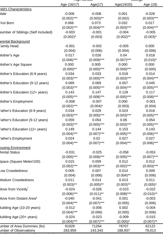
同年級小孩的讀書成效。結果我們發現，16 與 17 歲的青少年及 19 與 20 歲的

年輕成年人的學術表現與其家庭的住宅面積、居住時間與是否自有等變數有正且

顯著的關係；而與住宅年齡有負的關係。

在現在的國際學術文獻當中，本研究可能使用住宅資料來討論這個問

題最完整的文章，所以本文的學術貢獻應該是很可觀的，因此本文應該有很大的

機會在國際學術期刊上發表。

(2) 在本人發表的場次上，也有許多學者提出問題，顯示他們對於本

文的議題都很有興趣，對於本文的改進建議也有不少，對本文的修改也有很顯大

的助益。

六．

相關聯結：Faculty of Business Administration, University of Macau

http://www.umac.mo/fba

七．

附件：(1) 本人論文全文一份

(2) 大會手冊一份

New Evidence on the Link between Housing Environment and Children’s

Educational Attainments

+

Hsien-Ming Lien*, Wen-Chieh Wu**, Chu-Chia Lin***

Abstract

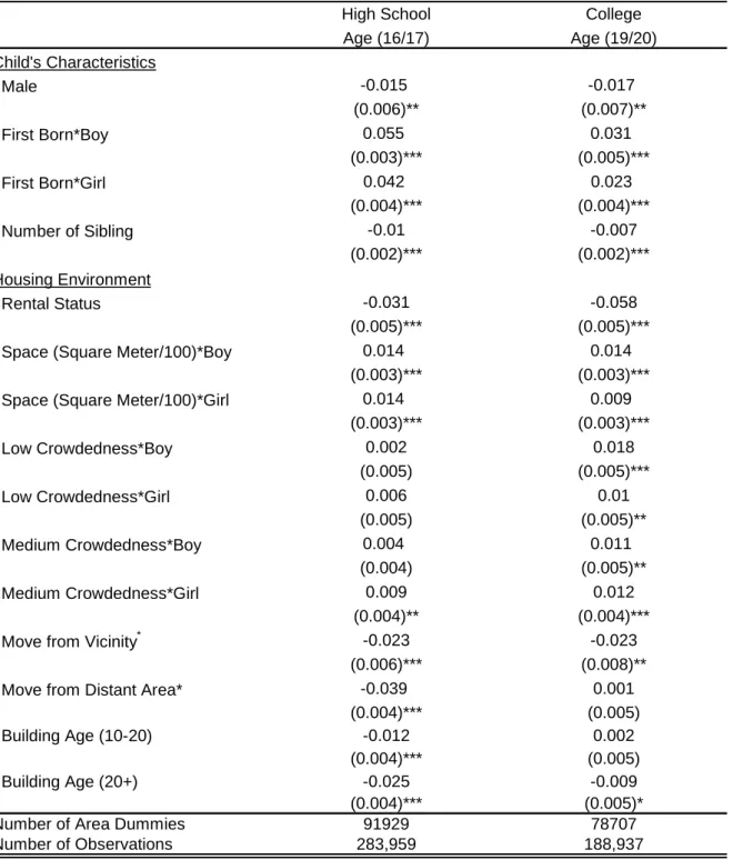
There is an extensive literature that posits the hypothesis that a better housing environment enhances a child’s educational attainments. However, there is little causal evidence demonstrating the presence of this effect. Using the census files covering the entire population of Taiwan, we examine the effect of housing environment on children’s educational attainments. Because the Taiwan census data contain unique address information for every household, we are able to control for unobserved family heterogeneity by comparing a child with his or her peers of the same age cohort in the same neighborhood. After controlling for neighborhood using tens of thousands of area dummies, the chance of high school enrollment for teens (ages 16 and 17) and college enrollment for young adults (ages 19 and 20) is found to be positively correlated with increases in floor space, increases in residential stability, and ownership status, but negatively correlated with increases in building age. In addition, we found that the effect of a child’s private space on the chance of school enrollment is nonlinear and different across age and gender. The results are robust even when we account for the potential endogeneity between sibship size and educational outcome using the instrumental variable method.

Keywords: quantity–quality trade-off, housing, educational attainment JEL classification: R0, I2

#

We thank David H. Autor, Charles Leung, and Jin-Tan Liu for their comments and suggestions. We are grateful to Directorate General of Budget, Accounting, and Statistics for providing the census data. Supports from National Science Council (NSC-93-2415-H-004-013) and National Health Research Institute (NHRI-EX93-9204PP) for Hsienming Lien are greatly appreciated. The usual disclaimer applies.

*

Department of Public Finance, National Cheng-Chi University, 64 Sec 2, Zhi-Nan Rd, Taipei, Taiwan; email:

[email protected].

**

Corresponding author, Department of Public Finance, National Cheng-Chi University, 64 Sec 2, Zhi-Nan Rd, Taipei, Taiwan; email:[email protected].

1. Introduction

One long-standing area of interest in the social sciences is to understand the connection between the family environment and a child’s outcome, particularly educational attainments. It is generally believed that a larger family size may negatively affect a child’s outcome through resource dilution [e.g., Blake (1981, 1989)]. The best-known economic theory that links family circumstances and a child’s educational outcome is perhaps the quantity–quality trade-off model [Becker and Lewis (1973) and Becker and Tomes (1976)]. This theory claims that as parents become richer because of the interaction between quantity and quality in the budget constraint, they demand higher quality children, but not necessarily more children. Thus, a reduction in family size leads to an improvement in a child’s schooling.

The majority of early studies confirm this trade-off relationship, with a negative relationship between family size and a child’s educational attainments being widely observed in regression results.1 While this negative correlation is often interpreted as evidence supporting the quantity– quality trade-off theory, the conclusions are facing serious criticism. Most problematic is that the apparent negative relationship is not necessarily indicative of a causal effect. That children raised in larger families have less schooling than those in smaller families is not necessarily because of the sibship size per se, but may reflect the omission of other unobserved characteristics, such as parental preferences, household resources, neighborhood conditions, and quality of schooling. In light of this potential bias, several studies have sought to uncover the causal effect of family size on a child’s educational outcome using the instrumental variable method (IV) [e.g., Angrist, Lavy, and Schlosser (2005), Caceres (2004), and Conley and Glauber (2005)], or controlling for family fixed effects [e.g., Guo and VanWey (1999) and Black, Devereux, and Salvanes (2005)]. Notably, these studies generally found the coefficient of sibship size becomes insignificant after controlling for unobserved family characteristics.

1

For a review in the economic literature on the link between family size and children’s outcomes, see Schultz (2005). There have also been numerous discussions on this issue in sociology. For details, see Blake (1981, 1989), Powell and Stellman (1993), and Guo and VanWey (1999).

Why are results of OLS estimation so different from those of IV or the family fixed effects model? One likely explanation, as pointed out by Phillips (1999), is that sibship size does not produce a negative impact on a child’s educational outcome, but the type of family resources it dilutes does.2 Furthermore, Goux and Maurin (2005) investigated the effect of household crowdedness on a child’s school performance, one key resource likely to affect a child’s education. Using exogenous variations of family size and household crowdedness as instruments, they found the importance of sibship size becomes negligible under IV estimation, but the private space each child has is negatively associated with a child’s educational attainments. In other words, children in large families perform less well not because of their family size, but because of the smaller private space each child has available to them.

In the same spirit as Goux and Maurin (2005), this paper seeks to explore the underlying relationship between the housing environment and a child’s educational attainments. Unlike Goux and Maurin (2005), which controls for unobserved family heterogeneity using instruments, we overcome this difficulty by comparing a child with his or her peers of the same age in the same very small neighborhood: “lin,” the smallest government jurisdiction in Taiwan that usually covers less than 0.1 square kilometer. Families residing in the same lin often share similar housing preferences and family incomes. In addition, youths raised in the same lin generally have experienced the same neighborhood effect. Furthermore, under the current regulation, children in the same lin typically attend the same school for compulsory education. Thus, by comparing youths with peers of the same age in the same lin, we control to some extent for unobserved family heterogeneity such as parental preferences, earning potential, neighborhood conditions, and, most importantly, quality of compulsory schooling.

Our data are derived from the census files that cover the entire Taiwanese population, more than 22 million, in the year 2000. The census data not only record detailed family and housing information, but also include unique address information for every household. The large sample size, together with detailed address information, allows us to examine the chances of high school enrollment for teens (ages 16 and 17) and college enrollment for young adults (ages 19 and 20) while controlling for family

2

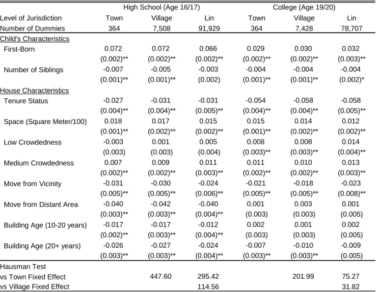
heterogeneity. After including tens of thousands of area dummies, our results confirm the importance of housing environment in determining a child’s educational attainments. Specifically, our estimates show that youths’ educational attainment is positively associated with an increase in housing floor space, an increase in residential stability, and ownership status, but negatively related to an increase of building age. The results continue to hold even accounting for the endogeneity between sibship size and a child’s education using twin births or sex-composition as instruments.

An important difference between our study and Goux and Maurin (2005) is that we include a wide range of housing variables. Aside from each child’s private space, this study also considers a house’s floor space, building age, residential stability, and ownership status as various determinants of housing environment. Therefore, the analysis is able to provide a more complete picture about the impact of housing on a child’s education. Another key difference is that we obtain a different effect of household crowdedness. While Goux and Maurin (2005) found that a reduction in a child’s private space resulted in a negative effect on his or her schooling, our estimates indicate that the effect may be nonlinear: conditional on a household’s size, reducing each child’s private space does not always lead to an decrease in the chance of school enrollment. Moreover, this crowdedness effect is likely to differ according to the child’s gender and age.

Our paper also relates to another line of literature exploring the effect of housing variables on children’s outcomes, including tenure status [e.g., Green and White (1997), Boehm and Schlottmann (1999), Aaronson (2000), and Haurin, Parcel, and Haurin (2002)] and residential mobility [e.g., Lee, Oropesa, and Kanan (1994), Green and White (1997), Aaronson (2000), and Haurin, Parcel, and Haurin (2002)].3 Although some studies have demonstrated the importance of housing environment, few of them controlled for the endogeneity problem caused by various housing variables.4 To our knowledge, this paper is the first study that investigates the effect on a child’s educational attainments of a wide range of housing variables.

3

For a complete review on the tenure status literature, see Haurin, Dietz, and Weinberg (2003).

4

A number of studies have attempted to control for the endogeneity of housing variables. For instance, Green and White (1997) adopted the bivariate probit model to solve the selection bias problem between tenure decision and schooling, but found no evidence of it. Haurin, Parcel, and Haurin (2002) used a treatment effect model to reduce selection bias. Aaronson (2000) dealt with the endogeneity problem of home ownership and mobility.

The paper is organized as follows. In the next section, we outline the estimation problem and discuss the existing identification strategies as well as our strategies. Section 3 describes the data source, sample selection, and measures of educational attainments, along with the basic statistics of our sample. Section 4 shows results of the basic specification, the effect of area dummies, as well as comparisons with IV estimates. Section 5 offers concluding remarks.

2. Conceptual Framework A. Parameter of Interest Let:

,

i i i i i

edu

=

X

α β

+

N

+ +

ν ε

(1)

where is the child’s educational attainments, is a vector of observed characteristics of the child and his or her family (e.g., age, sex, birth order, and father’s and mother’s education and working status), is a variable of child i’s sibship size, is the family-specific unobserved determinant (e.g., parental preferences or quality of schooling), and

i

edu

X

_i

i

N

v

_i

i

ε

represents the idiosyncratic shock that is assumed to be independent across other factors.

β

The central parameter of interest is , which is viewed as a measure of the trade-off between quantity and quality of children. Early studies primarily found this coefficient to be negative in OLS estimation and therefore inferred that substantial quality improvements can be gained by controlling for family size. However, the regression results are likely to be confounded by the existing observed factors (e.g., parental education) as well as the unobserved determinants (e.g., quality of schooling). The omitted variable formula suggests that the OLS coefficient from the regression is:

cov( , ) cov( , ) var( ) var( ) i i i i OLS i i N X N v N N

α

β

= +

β

+ (2) .

Therefore, even if children raised in larger families have less schooling than those in smaller families, the strength of the relationship could be driven by the correlation between sibship size and other observed and unobserved factors, not necessarily the quantity–quality trade-off.

B. Existing Identification Strategy

In light of the potential bias, the existing literature has adopted several methods to uncover the underlying relationship between a child’s education and sibship size. Early studies attempted to account for this potential bias by including more controls, such as parental IQ, and better measures of household income. However, adding more controls cannot rule out the possibility of an association between family size, educational attainment, and something immeasurable, such as housing environment, neighborhood conditions, or quality of schooling. As a result, recent studies have taken different approaches to account for unobserved family heterogeneity. For instance, Guo and VanWey (1999) and Black, Devereux, and Salvanes (2005) include the household’s dummies, i.e., family fixed effects, to control for the unobserved family-level heterogeneity. Angrist, Lavy, and Schlosser (2005), Caceres (2004), and Conley and Glauber (2005) employ exogenous variations in family size, such as multiple births or preferences of a mixed sibling-sex composition, as instruments to investigate the causal effect of family size on a child’s education. Notably, studies using IV estimations or fixed family effects found weaker correlations between family size and a child’s education, many of which turn out to be negligible.

The inconsistency of results between OLS and other estimation methods cast doubts over the link between family size and a child’s outcome. One likely explanation, as pointed out by Phillips (1999), is that sibship size per se does not affect the child’s educational attainments, but the type of resources it dilutes does. Goux and Maurin (2005) extended this line of thought by exploring the impact of a child’s private space, one important kind of resource likely to be affected by additional children, on the child’s schooling. Specifically, they considered the following equation:

,

i i i i i

edu

=

X

α β

+

N

+

γ

h

+ +

ν ε

i

where is the average number of rooms per person in the household, used as a proxy for a child’s private space. Notice that equation (3) also includes the sibship size variable to account for the effect caused by family size. Because sibship size and the child’s private space are likely to be endogenous, they employ two instruments, gender of the first two children and of the last two children, respectively, to control for unobserved family heterogeneity. Consistent with previous studies, they found that the coefficient of sibship size becomes insignificant under IV estimation. Interestingly, the coefficient of the average number of rooms per person in IV estimates is significantly negative, suggesting that children in large families perform less well, not because of their family size, but because of the smaller private space available to each child.

i

h

C. Our Identification Strategy

In contrast to Goux and Maurin (2005), our study seeks to identify the effect of a variety of housing variables on a child’s educational outcome, such that:

.

i i i i i

edu

=

X

α β

+

N

+

H

γ ν

+ +

ε

_i (4)

The biggest difference between (3) and (4) is that the housing environment is now a vector of multiple variables ( ) instead of a single variable ( ). There are substantial difficulties in using existing identification strategies for this specification. Because these housing variables do not change within a household, including household dummies essentially eliminates the effect of housing environment. Another possible strategy is to find instruments for housing variables, as Goux and Maurin (2005) did for household crowdedness. Nevertheless, controlling for the unobserved heterogeneity in this setting requires us to find many more instruments.

i

H

h

_i

We take a different approach to identify the causal link. Apart from including a detailed set of important variables of a child’s family background used in previous studies (e.g., a child’s birth order, parental age, work status, and education), we account for unobserved family heterogeneity by adding dummies of the child’s residential neighborhood. Our unique data are derived from the census data

Therefore, we are able to compare a child with his or her peers of the same age in the same very small neighborhood, the lin. Families residing in the same lin tend to share similar housing preferences and parental incomes, as well as earning potentials. Moreover, youths raised in the same lin generally encounter the same neighborhood effect. Furthermore, youths in the same lin typically attend the same elementary or junior high schools, allowing us to control for the quality of compulsory schooling prior to high school or college. In fact, given Taiwan’s current school regulation, it is almost certain that youths in the same lin go to the same school.5,6 Thus, by controlling for neighborhood fixed effects, we account for the neighborhood effect, quality of schooling, and parental incomes and preferences. Nevertheless, it is still possible that our approach may not fully capture unobserved family heterogeneity. We will discuss this point in the results section.

To be more specific, we estimate the following equation:

i

,

i i i i i

edu

=

X

α β

+

N

+

γ

H

+

Area

+

ε

(5)

where is a dummy equal to one if child i’s highest educational attainment is general high school for teens or general college for young adults, and zero otherwise; is a set of variables on the housing environment, including building age, tenure status, household crowdedness, and residential stability; is a vector of neighborhood dummies to control for unobserved family heterogeneity; and i

edu

i

H

i

Area

i

ε

is an independent error across various individuals. As discussed earlier, we compare youths residing in the same lin. In Taiwan, the lin is the fourth and smallest level of government jurisdiction, following county, town, and village. As such, the estimation includes tens of thousands of area

5

According to Taiwan Compulsory Education Law, students residing in the same “lin” belong to the same public school district and thus are assigned to the same public elementary or junior high school. For instance, the school district for Beitu Elementary School in Taipei includes every Lin of Central and Da-Tong Villages, 1st–9th and 12th Lin of Chang-An, 2nd Lin of Hot-Spring Village, and 1st–10th Lin of Ching-Jiang Village. For details on the regulations, see http://www.tp.edu.tw/neighbor/elementary/e_beitu.jsp.

6

One exception is that children hoping to enroll in better elementary or junior high schools may move their registries to relatives or friends residing in better school districts, but continue to live with their parents. In this case, those children are coded as “other relatives” in the households of friends or relatives in the census. Because our data remove children that coreside with other relatives, we expect this proportion to be small in our sample.

dummies. Because of computational complexity, we focus on the linear probability model instead of nonlinear models. Alternative models (e.g., probit and logit), however, yield similar results.

3. Data and Sample

A. Data Source

The data for this study are derived from the 2000 Taiwan census, conducted every 10 years by the Directorate of General Budgeting, Accounting, and Statistics. The Taiwan census files collect information using a detailed questionnaire similar to that used to create the PUMS files for the US censuses (long-form), except that income-related variables are excluded. At each household, the interviewer records each individual’s basic demographics (race, sex, age, and marital status), educational attainment, relationship with the head of household, working and employment status within the past two weeks, as well as the industry in which he or she works. In addition, the interviewer records the residence’s structure (number of living rooms, bedrooms, kitchens, and bathrooms), tenure status (rent or own), years lived in the residence, and the location from which the family last moved. The residence information is further linked with the housing registry from the Ministry of Interior to ascertain the floor space of the house, the building year, and the major construction material used for the residence. More importantly, the Taiwan census includes a scrambled, but unique, address for every household’s residence. As seen below, this unique address information plays an essential role in the analysis.

The advantage of using the Taiwan census is that the files contain the full sample of Taiwan residents, around 22 million in total or 300,000 individuals in most age cohorts. The large sample size, together with the detailed address information, provides a good opportunity to analyze the effect on educational attainment of the housing environment. Ideally, we would examine the link using the final education levels of all family adult respondents and their current housing information. In practice, however, this is not possible because the census files do not record family information of those who no longer reside with their parents and siblings. Obtaining the complete family background is therefore difficult, especially for adult respondents because a large portion of them do not coreside with parents

and siblings. Moreover, the census files report only the respondent’s relationship with the head of the household, but not with other members. Although we could match their relationships according to each member’s age and gender, the identification becomes quite complicated when there are more than three adults in a household (e.g., coresiding with a brother or sister-in-law).

B. Sample Selection

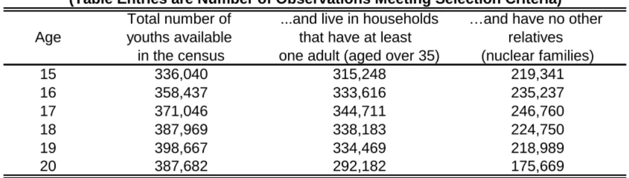
For the purposes of this study, we restrict the sample in several ways. We select households with at least one unmarried child aged between 15 and 20 at the time of the census, of which the eldest sibling is no older than 22. We focus on the younger sample to reduce the bias resulting from incomplete family information. We restrict the sample to ages over 15 because compulsory schooling in Taiwan ends at junior high school (9th grade). To avoid mistakes arising from matching parents, we keep only nuclear families in the sample, eliminating households that live with grandparents, relatives, or other friends. Furthermore, we drop households in which children are raised by a single parent to reduce complications because different family structures may also affect a child’s education. Finally, we include only samples that have stayed in the residence for at least three years because the housing effect usually takes a longer time to materialize.

To demonstrate the impact of exclusion criteria, Table 1 lists the observed number of youths aged from 15 to 20 for each selection criteria. The first column lists the total number of youths in the census by age cohort. As indicated by these numbers, the number of respondents peaks at the age of 19 and then gradually declines as their age rises; this pattern is consistent with the number of births between 1980 and 1985 (ages 15 to 20 in 2000) in Taiwan.7 The vast majority of youths, particularly younger ones, coreside with their families. This can be seen from the difference between the first and the second columns, which shows the number of youths who live with at least one adult aged 35 or older. Nevertheless, more and more youths, especially those older than 20 years, choose to live alone for either marriage or work reasons. That youths live alone for other reasons may increase the risks of matching complete family information, a point we will return to later.

7

The number of respondents obtained from the census data is very close to the birth numbers between 1970 and 1975; the difference is less than 3 percent in every age cohort.

The largest reduction in sample size occurs when restricting the sample to nuclear families. This is not surprising because about 67% of the elderly in Taiwan coreside with their children.8 Among these nuclear families, around 20% of the youth do not have valid parental information: either they are growing up in single-parent families (around 60% are single mothers) or are no longer coresiding with both parents. Another 10–20% are removed because of the age restriction of the eldest sibling; the older the respondent, the more likely they are to be removed by this age constraint. Finally, around 7% are eliminated because they have stayed in the current residence for less than three years. The final sample size consists of a little over one third of the original sample. Still, we have around 100,000 respondents in each age cohort.

C. Measure of Educational Attainment

Before describing our analysis sample, it is important to first discuss our measures of educational attainment. Previously used measures include the highest completed level of education [Boehm and Schlottmann (1999), Angrist, Lavy and Schlosser (2005), Black, Devereux and Salvanes (2005)], private school attendance [Conley and Glauber (2005)], held back in school grade [Conley and Glauber (2005), Goux and Maurin (2005)], test scores [Guo and VanWey (1999), Haurin, Parcel, and Haurin (2002)], dropping out [Green and White (1997)], and graduating from school by a certain age [Aaronson (2000)]. Because our data are derived from the census files, we cannot make distinctions between the quality of the youth’s school (e.g., school ranking), or the youth’s academic performance within the school. Therefore, we adopt a measure similar to the one used in Conley and Glauber (2005) that compares the respondent’s age with the highest schooling that he or she is currently enrolled in or has completed so far. The education system in Taiwan is similar to that of the United States, except that compulsory schooling is nine instead of 12 years. Therefore, from the age of six, children are required to take six years of elementary school and three years of junior high school. After finishing junior high school, those seeking additional education can go to senior high school (three years) and even higher after graduating from high school. Suppose a child of age 16 reports his or her highest