Adaptive Brain-computer Interface using
Motor-imagery EEG
A thesis presented byShih-Wei Lu
toInstitute of Computer Science and Engineering
College of Computer Science
in partial fulfillment of the requirements for the degree of
Master
in the subject of
Computer Science
National Chiao Tung University Hsinchu, Taiwan
Copyright c 2007 by
Abstract
Recently, the research of EEG-based Brain-computer Interface provides a new way of communication and control. In the existing BCI researches, we are interested in the motor-imagery based BCI systems. Nowaday this kind of BCI system is facing many challanges such as noises and inter-subject variability. There are many issues to study, the noise reduction, the adaptation between a BCI and a user, the feedback of the BCI, etc.
In this work, we studied the adaptation issue in the Brain-computer Interface based on the motor-imagery EEG. First, we want to construct a good spatial filter that suppresses the noises and enhances the power change in a motor-imagery task. We use Maximum Contrast Beamforming technique to construct the spatial filter. This technique has its ability to lower the nontarget noise and enhance the contrast between the active state and control state we define. We focus on the usability of this spatial filter and analyse its performance by applying a ROC curve analysis. In this work we show that this spatial filter has its effectiveness.
Furthermore, we applied the constructed spatial filter online. We designed a two-session online experiment with a visual feedback to study the adaptation and the biofeedback is-sues. We expect the user to adapt himself to the system by monitoring the visual feedback, and the system to adapt to the user by training a new spatial filter. The result tells us that the spatial filter is possible to work online, but the visual feedback somehow affects the ERS in the motor-imagery tasks.
Acknowledgements
Contents
List of Figures vii
List of Tables ix
1 Introduction 1
1.1 Motivation . . . 2
1.2 The Human Brain . . . 3
1.3 Electroencephalography . . . 4
1.3.1 What is Electroencephalography . . . 4
1.3.2 How to measure Electroencephalography . . . 4
1.3.3 Basic Analysis to Electroencephalography . . . 5
1.4 Brain-computer Interface . . . 8
1.5 Thesis Overview . . . 9
2 Overview of Brain-computer Interface 11 2.1 Categories of Brain-computer Interface systems . . . 12
2.2 Basic Components in BCIs . . . 12
2.3 Present-day BCI systems . . . 14
2.3.1 ERP-based BCI . . . 14
2.3.2 Motor-imagery based BCI . . . 15
2.4 Limitations . . . 16
2.5 Key-issues in BCI systems . . . 17
2.6 Thesis scope . . . 19
3 Cortical activity analysis for BCI 21 3.1 Main ideas . . . 22
3.2 Data acquisition and preprocessing . . . 22
3.3 Time-frequency analysis . . . 23
3.4 Spatial filtering . . . 24
3.4.1 Introduction . . . 25
3.4.2 Beamforming technique . . . 25 v
3.5.1 ROC curve analysis . . . 31 4 Experiments 33 4.1 Offline analysis . . . 34 4.1.1 Experiment setup . . . 34 4.1.2 Data analysis . . . 36 4.1.3 Experiment results . . . 37
4.2 Online feedback experiment . . . 54
4.2.1 Experiment setup . . . 54
4.2.2 Experiment results . . . 56
4.3 Observations . . . 57
5 Discussion 59 5.1 Spatial filter . . . 60
5.1.1 Stability of the spatial filter . . . 60
5.1.2 Different selection of control/active state . . . 64
5.1.3 Comparison between MCB and CSP . . . 66
5.1.4 Number of training trials . . . 68
5.2 Adaptation . . . 75
5.2.1 The system to user adaptation . . . 75
5.2.2 The user to system adaptation . . . 76
5.3 Limitations . . . 76
6 Conclusions and Future Works 79 6.1 Conclusions . . . 80
6.2 Future works . . . 81
Bibliography 85
List of Figures
1.1 The lobes of human brain . . . 3
1.2 The functions of different cortex areas . . . 4
1.3 EEG measuring devices . . . 5
1.4 The international 10-20 system . . . 6
1.5 The P300 ERP . . . 7
1.6 The procedure of observing ERD/ERS . . . 8
1.7 Movement related alpha ERD and ERS . . . 9
1.8 The general flowchart of a BCI . . . 10
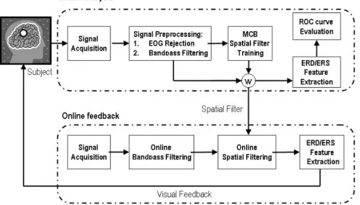
2.1 Flowchart of proposed BCI . . . 20
3.1 Example of a time-frequency map . . . 24
3.2 The concept of spatial filtering . . . 25
3.3 ROC curve analysis . . . 31
4.1 Experiment paradigm . . . 35
4.2 Time-Frequency map of Subject A, Experiment 1. . . 38
4.3 ERD/ERS curve of Subject A, Experiment 1. . . 38
4.4 Time-Frequency map of Subject A, Experiment 2. . . 39
4.5 ERD/ERS curve of Subject A, Experiment 2. . . 39
4.6 Time-Frequency map of Subject A, Experiment 3. . . 40
4.7 ERD/ERS curve of Subject A, Experiment 3. . . 40
4.8 Time-Frequency map of Subject A, Experiment 4. . . 41
4.9 ERD/ERS curve of Subject A, Experiment 4. . . 41
4.10 ROC curve analysis of Subject A, imagery session 1 and 2 . . . 42
4.11 ROC curve analysis of Subject A, imagery session 3 and 4 . . . 42
4.12 Time-Frequency map of Subject B, Experiment 1. . . 44
4.13 ERD/ERS curve of Subject B, Experiment 1. . . 44
4.14 Time-Frequency map of Subject B, Experiment 2. . . 45
4.15 ERD/ERS curve of Subject B, Experiment 2. . . 45
4.16 Time-Frequency map of Subject B, Experiment 3. . . 46
4.17 ERD/ERS curve of Subject B, Experiment 3. . . 46 vii
4.20 Time-Frequency map of Subject C, Experiment 2. . . 49
4.21 ERD/ERS curve of Subject C, Experiment 2. . . 49
4.22 Time-Frequency map of Subject C, Experiment 5. . . 50
4.23 ERD/ERS curve of Subject C, Experiment 5. . . 50
4.24 Time-Frequency map of Subject D, Experiment 1. . . 52
4.25 ERD/ERS curve of Subject D, Experiment 1. . . 52
4.26 Time-Frequency map of Subject D, Experiment 2. . . 53
4.27 ERD/ERS curve of Subject D, Experiment 2. . . 53
4.28 Online experiment paradigm design . . . 54
4.29 Online experiment visual feedback . . . 54
4.30 ERD/ERS curve of Subject A, Experiment 1. . . 56
5.1 Different result when choosing different active/control state . . . 65
5.2 C4 channel data compared to CSP and MCB filtered data, subject A im-agery session 1 and 2 . . . 69
5.3 C4 channel data compared to CSP and MCB filtered data, subject A im-agery session 3 and 4 . . . 70
5.4 Trial number vs. filter performance analysis . . . 71
5.5 Result of different onset time of the visual feedback . . . 75
List of Tables
4.1 Results of subject A imagery movement . . . 43 5.1 Correlation coefficients between different sessions, wrist real movement,
subject A . . . 61 5.2 Correlation coefficients between different sessions, wrist imagery
move-ment, subject A . . . 62 5.3 Correlation coefficients between different tasks, subject A . . . 63 5.4 Correlation coefficients between different subjects . . . 64 5.5 Results of different selection of control/active states, subject A real movement 72 5.6 Results of different selection of control/active states, subject A imagery
movement . . . 73 5.7 Trial number analysis using dataset 4 of subject A . . . 74 5.8 Trial number analysis using dataset 3 of subject A . . . 74
Chapter 1
Introduction
In this first chapter we give some background knowledge to this thesis. We briefly introduce from the human brain to Electroencephalography to Brain-computer Interfaces. In section 1.2 we introduce the structure of a human brain and the different functions of cortex areas. In section 1.3 we give some introduction to Electroencephalography (EEG), so called brain wave. The measurement way, some basic analyses and researches are pre-sented. In section 1.4 we give a brief introduction to Brain-computer Interfaces (BCI). The detail of BCI systems will be provided in the next chapter.
1.1
Motivation
There are a lot of patients suffering from the paralyzed body. Disorders such as Spinocere-bellar Ataxia (SCA) and Amyotrophic Lateral Sclerosis (ALS) are motor-disabled. These diseases make the patients unable to communicate with the external world through the nor-mal pathway. They can’t talk or move their fingers to click a button.
As the time is different now, we start to think about the other pathways between human and a computer. That is, a Brain-computer Interface. A Brain-computer interface is defined as a communication system that does not depend on the brains normal output pathways of peripheral nerves and muscles. Nowadays researchers use Electroencephalogram, so called brain wave, as a source to communicate and control. The users can use a Brain-computer interface to communicate with the outside world without using any real movement. So if this technique successes, it indeed helps lots of motor-diabled people. Even if those are not paralyzed, the BCI system may provide some assistance to some works, like moni-toring a pilot’s fatigue to avoid accident, or monimoni-toring a child’s brain waves to train his concentration.
So researchers keep doing researches on EEG and BCI. The more we discover about the human brain, the more people we may help in the future.
1.2 The Human Brain 3
Figure 1.1: The lobes of human brain. [6]
1.2
The Human Brain
The human brain can be divided into four structures: cerebral cortex, cerebellum, brain stem, hypothalamus and thamalus. The one that related to BCIs is the cerebral cortex. The cerebral cortex can be divided in two hemispheres, left and right. And each hemi-sphere can be further divided into four lobes. The four lobes are frontal lobe, parietal lobe, temporal lobe, and occipital lobe, as figure 1.1 shows. The cerebral cortex is responsible for many complicated functions like mental calculating, language learning, visual stimulus processing, or motor movement. The different areas in the cerebral cortex are responsible for different functions. As figure 1.2 shows, these different areas of cerebral cortex are marked with different colors, indicating its responsible functions. For instance, the motor area is located at about parietal lobe. It’s responsible for all the movement of the body. These informations are very important when doing researches on a EEG based BCI sys-tem. We observe the EEG from different locations on the head according to that area’s representative function. For instance, we observe mainly the EEG from the channels lo-cated on the top(parietal) of the head when we are doing motor-related experiments, and we observe mainly the channels on the back(occipital) of the head when we are researching about visual stimulus.
Figure 1.2: The functions of different cortex areas. [4]
1.3
Electroencephalography
1.3.1
What is Electroencephalography
Electroencephalography. There exists various non-invasive techniques to monitor the brain activity such as functional Magnetic Resonance Imaging (fMRI), magnetoencephalog-raphy (MEG), and Electroencephalogmagnetoencephalog-raphy (EEG). EEG is used to measure the electrical activity of the brain. This activity is generated by billions of nerve cells, called neurons. Each neuron is connected to thousands of other neurons, and the neurons send action po-tentials to other neurons when they are communicating. When we measure the EEG, we actually are measureing the combined electrical activity of millions of neurons on the cere-bral cortex because the potential of a single neuron is too small to be measured.
1.3.2
How to measure Electroencephalography
How to measure human EEG and record it for analysis? A typical EEG meauring device consists of several components, including EEG electrode cap that receives the electrical avtivity from the scalp, EEG amplifier that amplifys the signal, computers that record the data, and monitors that give the subjects visual cues. The devices are shown in figure 1.3.
1.3 Electroencephalography 5
Figure 1.3: EEG measuring devices. From right to left is the EEG amplifier and the elec-trode cap.
which depends on the electrode number of an EEG electrode cap. The electrode layout on an EEG electrode cap has a international standtard called the international 10-20 system, as figure 1.4 shows. When we are measureing EEG, we often put some single electrodes surrounding the eye. This is used to measure the electrical activity of eye movement and eye blinking, which is called EOG. This EOG contaminates the EEG signal badly, so by measuring it we can remove the trials that was affected. This processing is called EOG rejection.
When we use an EEG electrode cap to measure EEG, we have to fill each electrode with the electrolyte gel using a blunt needle. This makes the electrodes contact the scalp and lower the impedance. In an EEG experiment we often wait until all the electrodes have an impedence lower 5k ohm before we start the signal acquisition.
1.3.3
Basic Analysis to Electroencephalography
There are some basic EEG analyses, mainly described here as time domain and fre-quency domain analysis.
Time domain analysis
Usually we use time domain analysis to observe an Event-related Potential (ERP). An ERP is a potential change in the EEG when a particular event or stimulus occurs. The
Figure 1.4: The international 10-20 system. The 10 and 20 means 10% and 20% distance in the left figure. The channels are named as a capital letter followed by a number. The capital letter ’F’ is for ’Frontal, ’C’ is for ’Central’, ’P’ is for ’Parietal’, ’O’ is for ’Occipital’, and ’T’ is for ’Temporal’. The numbers are odd on the left sphere and even on the right sphere. [5]
potential change is time-locked and phase-locked, it is a very small potential change and can not be easily observed in a single trial. So we have to average a few trials to observe it. Because of the time-locked and phase-locked characteristic, by the averaging technique we can eliminate the random noise and enhance the signal-to-noise ratio (SNR). That is the common technique to observe an ERP.
There are some well-known ERPs, including P100 in the Visual-evoked Potential (VEP), P300, N400, and Audio-evoked Potential (AEP). The P300 means a positive potential change occers 300ms after the particular stimulus, as figure 1.5. In section 2.3.1 we will introduce more about the application on BCIs using ERPs.
Frequency domain analysis
In addition to the ERPs in time domain analysis, we can observe Event-related Syn-chronization (ERS) and Event-related DesynSyn-chronization (ERD) in the frequency domain. When we are observing ERD and ERS, we have to observe a spicific frequency band, like alpha band (8-12Hz) or beta band (around 20Hz). The ERD and ERS indicate the power changes of the frequency band. While ERD means the power decreasing and ERS means the power increasing.
1.3 Electroencephalography 7 o ther c ho ic e d es ired c ho ic e
P z
Figure 1.5: The P300 ERP. 300ms after the particular stimulus, there is a positive potential change in the time domain. This figure is a result of averaging. [3]
1. First we apply a bandpass filter with a spicific frequency band to the data. 2. Calculate the mean of the filtered data over all trials.
3. Subtract the mean from the filtered data in step1.
4. We do the squaring on the time domain amplitude samples from the previous step over all trials.
5. Average over time samples from the step4.
6. Obtain ERD/ERS by calculating the percentage relative to the power of the baseline interval.
Then we can see the power change and the change rate clearly after these procedures. There are some well-known ERD/ERS. For example, the movement related ERD and ERS. It it known by now that during the movement there is an alpha ERD, and after the movement terminates there is a beta ERS. In this thesis we are mainly observing this phe-nomenon. Figure 1.7 shows the movement related alpha ERD and ERS. In addition to observing the ERD/ERS curve, we can analyse the data using wavelet transform to obtain a
Figure 1.6: The procedure of observing ERD/ERS. [14]
time-frequency map. This analysis contains more information, we use this technique much in this thesis. The ERD/ERS issue is very important in a motor-related BCI. As for this thesis, we are trying to enhance the ERD to ERS ratio in a wrist imagery movement task. The details will be described in section 3.4.3.
1.4
Brain-computer Interface
Over the past few decades, the EEG has beenused mainly for evaluation of neurolog-ical disorders in the clinic and for the investigation of brain functions. Until recently, re-searchers found it possible to translate some specific EEG to commands. That is, people can communicate with others or control devices directly by their brain activity, without using any normal pathways of the peripheral nerves. This communication and control technique
1.5 Thesis Overview 9
Figure 1.7: Movement related alpha ERD and ERS. The cue point was a visual cue indi-cating the subject to perform hand movement. When the movement is proceeding, there is an ERD, and when the movement terminates, there is an ERS.
was then called Brain-computer Interface.
A Brain-computer interface is defined as a communication system that does not de-pend on the brains normal output pathways of peripheral nerves and muscles. Among the methods to measure electrical activity, MEG and EEG are more suitable for a BCI system because they can give the instantaneous continuous recording of brain activity. And EEG is even more suitable because of the following advantages: the devices to measure EEG are more portable and cheaper, and we don’t have to be in a shielding room when measuring EEG. Although the EEG signal is having low spatial resolution compared to the others. Almost all BCI researches are using EEG signal nowadays.
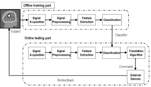
A general BCI flowchart is as figure 1.8 shows. The BCI system goes through the data acquisition, then some signal processing, followed by a command translation, in the end output commands to communicate with others or to control cursors or devices. The details of a BCI system will be described in the next chapter.
1.5
Thesis Overview
Chapter 2 provides the overview of BCI systems, including the basic components and key-issues. We also introduce some present-day BCIs here. The methods used in our BCI will be introduced in Chapter 3. We mainly want to design and test an optimal spatial filter to filter the data. With the noise suppressed and features enhanced, we can obtain
Figure 1.8: The general flowchart of a BCI.
significant data for further classification. Chapter 4 provides the experiment results of our designed offline experiments. We show the analysis results of the spatial filter along with some further performance evaluation results. In chapter 5, we show the experiment results of online feedback sessions and give some brief discussion. In chapter 6 and 7 we give this thesis some conclusion and detailed discussions, including the stability of our spatial filter, the feedback issue, the adaptation issue, and the future works.
Chapter 2
In this chapter we will give an overview to BCI systems. We first introduce some categories of BCI systems, then we briefly introduce some present-day BCIs. Next we list and explain some basic components and nowaday key-issues in a BCI system. In the end of this chapter we provide the thesis scope.
2.1
Categories of Brain-computer Interface systems
Synchronous and asynchronous systems
In a synchronous BCI, the user is notified to perform a mental activity when a specific external cue is shown. That means this kind of system operates in a cue-based mode and has the information about the onset of the mental activity in advance. The analyses and classification of the brain signals in the system is limited to the predefined fixed time pe-riod. Besides, the system is active only during the predefined period as well. BCI systems based on evoked potentials and ERPs belong to this category, such as P300 [2], SCP [8]. Besides EPRs, the BCI developed in Graz [15] that analyzed the spontaneous EEG are also synchronous BCIs.
The BCI that a user can intend a mental activity whenever he wishes to perform such mental activity is an asynchronous BCI. In the asynchronous BCI, the brain signals are an-alyzed and classified continuously. We have to not only classify from the redefined mental tasks but also discriminate events from noise and nonevents such as resting or idling states. Such a BCI system is more flexible and attractive to be utilized in practice. Besides the above advantages, it also offer a rapider response time than synchronous ones. However, the classification in an asynchronous BCI system is not accurate enough today.
2.2
Basic Components in BCIs
Signal pre-processing
The goal of the stage is to enhance the signal-to-noise ratio. Typical procedures include amplification, filtering, possible artifact removal. For the filtering, the bandpass filtering is usually applied. In addition, a notch filter is also used to suppress the 60 Hz power line
2.2 Basic Components in BCIs 13
interference. As for the artifact removal, almost all BCIs rule out the signals if the EOG or EMG is detected to be used or over a predefined threshold.
Feature Extraction
In this stage, certain features are extracted from the preprocessed signals. ERP, ERD/ERS and brain rhythms are typically used features in a BCI system. Besides the above features, various feature extraction methods have been studied to extract more discriminative fea-tures, such as Common Spatial filter, continuous wavelet transform, autoregress model(AR) or adaptive autoregress(AAR) model, power spectrum. All the above methods can be found in BCI competition 2003 papers.
Classification
The features extracted from feature extraction are fed to train a classifier. Many clas-sification methods have been proposed in pattern recognition field. The classifier in a BCI can be anything from a simple linear model to a complex nonlinear or a machine learning models. In general, the BCI has two phases training phase and testing phase. The training phase consists of a repetitive process of cue-based mental tasks to train a classifier. In the testing phase, we use the classifier built in the training phase to recognize different mental tasks.
Command Translation
The goal of this step is to translate the classification output in previous step to an oper-ator command. The command can be, e.g.,a letter in a spelling system or a movement of a course on the user’s screen or nothing to be performed when the classification is ”rest-ing” or ”idle”. The design of translation algorithm and device control depends on what applications the BCI want to provide with.
Biofeedback
A feedback which make the user more easily adaptive to the system is a very important component for a BCI system. A feedback can indicate how well the asked mental activity
was recognized by the system. When the system gives the feedback to a user, he will create a biofeedback which is the process that the user receives information about his biological state.
By Biofeedback, the user can monitor his physiological states, shape his brain electrical behavior, and voluntary modification of his EEG response. Today, nearly all BCI systems provide a feedback to users.
2.3
Present-day BCI systems
Here we introduce some present-day BCI systems, we mainly introduce two kinds of BCI systems, the ERP-based BCI and the motor-imagery based BCI.
2.3.1
ERP-based BCI
The details about ERP is described in section 2.3.1, because the ERP is evoked by the external events, this kind of BCI usually depends on the gaze of the user. We can always detect the ERP as long as we have enough trials. This kind of BCI has its advantages like the short training time and high accuracy. The drawbacks are the transition rate may be slow and the users may habituate to the system and lower the performance. Here we introduce two main ERP-based BCI, the P300-based and SSVEP-based BCI.
P300-based BCI
Farwell proposed a spelling BCI system based on P300 ERP [3]. In this system, users are gazing at a 6x6 matrix on the screen. In the matrix there are letters, numbers, and symbols. When the system starts, it flashes each row and column in the matrix with random sequence. The user is asked to focus his attention on the symbo he wants to select and count the number of time that this symbol is flashed. This is an oddball paradigm and the there will be an evoked P300 when the selected symbol is flashed. With enough trials, the system can predict the selected symbol by detecting the P300 response. That’s the concept of this BCI system.
2.3 Present-day BCI systems 15
SSVEP-based BCI
The SSVEP is Steady-state Visual Evoked Potential. It is a response to a visual stimulus with a specific high frequency. The EEG signal power will increase at the specific stimulus frequency. Therefore with some different frequency stimulus on the screen we can detect which one has the user’s gaze. There are lots of BCI application using SSVEP, such as Lalor [9], his team deveoped a game to balance a character on the screen using SSVEP.
2.3.2
Motor-imagery based BCI
Compared to the ERP-based BCI, the motor-imagery based BCI is more independent. This kind of BCI basically no need to depend on the user’s gaze. The motor-imagery is a spontaneously induced EEG signal. Therefore this kind of BCI is more difficult to develop since the imagery and the concentration of each user may be different. This kind of BCI has its advantages like high transition rate, and users may improve the performance through constant training. The drawbacks are, the training time is longer than a ERP-based BCI, and the user’s concentration is very improtant. Here we introduce the Graz group. [13]. The leader of this group is Dr. Gert Pfurtscheller. This group is in the Graz University of Technology in Austria. The Graz BCI is one of the most successful BCI using motor-imagery tasks. The development is mostly based on the detection of the ERD and ERS pattern in a motor-imagery task. Actually the concept of ERD and ERS was proposed by Pfurtscheller [14]. In their works there are lots of research about different movement that causes different kind of ERD and ERS. They’ve found some movement related ERD and ERS [14] such as:
• pre-movement alpha ERD
Different voluntary movement will induce an alpha band (8-12Hz) ERD in the cor-responding area of motor cortex. The study shows that this alpha ERD starts 1 or 2 seconds before the movement onset. The alpha band power keeps decreasing until the movement terminates. Then there is a ERS after the execution of movement. This ERS is seen as a recovery of the pre-movement ERD.
Same as the alpha ERD described above. The study shows that there exists a beta band (16-32 Hz) ERS after the movement terminates.
Today this group is focus on the feature extraction of the ERD and ERS pattern and the clas-sification of different movement imagery. The intend to classify left/right hand movement imagery, foot movement imagery, or tongue movement imagery. They use spatial filter as Common Spatial Pattern (CSP) or morlet wavelet transforms to extract the features. Fur-thermore they try Support Vector Machine (SVM) or Linear Discriminant Analysis (LDA) in the classification part.
2.4
Limitations
Although the BCI systems we introduced above looks well, there are still some lim-itations in present-day BCI systems. Here we list some normal difficulties when doing researches on BCI systems.
Habituation
In a ERP-based BCI 2.3.1, we use the evoked potential from the subejcts to develop a BCI system. For the evoked potential is not controlled by our own will, we may get used to the BCI system and that affects the performance. Take P300-based BCI for example, if a user use the BCI system day after day, year after year, he/she may habituates to the BCI, and his/her P300 response therefore reduces. This kind of habituation restricts the BCI systems that relys on the ERP responses.
Noise
As we mentioned before, the EEG signal is poor on the Signal-to-noise ratio. The artifact noise is always a big problem in analysing EEG signals. Eye blinking, eye move-ments, the heart beating, any possible single small movement causes artifact noises to the EEG signal. Furthermore, not only an artifact causes noises. The interference from the environment, the power line, or the devices, they are also contaminating the EEG signal. In a BCI system, we detect the spontaneous EEG signals or the evoked potential. Both are
2.5 Key-issues in BCI systems 17
very small changes and can be easily affected by these noises. In addition to the artifacts and interference, a distraction of the user also causes noises to the EEG signal. As a hu-man being is very complicated, every little cognitive task has its own response on the EEG signal. We can’t be sure that every user of the BCI system are always concentrating to the system, one may easily lose concentration and that reduces the performance of a BCI.
Fatigue
Another limitation to BCI systems is the fatigue of the users. As we introduced in the previous section, the ERP-based BCI keeps giving stimulus to the users and detect their responses. These stimuli may be some quickly changed pictures or flashing, and these fatigue a user easily. Even if in a motor-imagery based BCI, the users may get tired easily because of the continuous concentrate on the imagenery.
2.5
Key-issues in BCI systems
Here we list some key-issues in BCI systems. The future researches on BCI systems may be mostly about these difficult issues.
Noise Reduction
As we mentioned in the previous section, the noise is a limitation to the EEG analyses and BCI systems. How to reduce the noise and the non-interested signals is an issue. Today there are some practical methods to reduce the noises, such as EOG rejection, bandpass filtering, Independent component analysis (ICA), or Laplacian spatial filtering. In this thesis, we designed a spatial filter to filter the data. The filtered data suppresses the non-target noises and enhanced the motor-imagery induced responses. We’ll discuss this in the next chapter.
Features
How to find significant features from the EEG signal is an important issue. People have been trying with many methods to extract significant features from the raw EEG data. In
this work, we use the designed spatial filter to suppress the noise and enhance the power change in the signal. Like the CSP [11] method, we can view our spatial filtering approach as feature extraction.
Adaptation
There are two adaptation issues in a BCI system. The first is the users should adapt themselves to the system, that is, self-training of the users. The second is, the BCI system should adapt itselves to the users, that is a machine learning issue. Both adaptation issues are important, and these two issues work totally different. If we are trying to self-training a user, we should lower the variability of the BCI system, or the users may not be able to get himself trained well because the feedback keeps changing. The training of the users is still a difficult question. In this work, we use a online visual feedback experiment to observe this user adaptation issue, we’ll discuss this in chapter 5.
Biofeedback
As we mentioned before, the biofeedback is a important component in the BCI sys-tem. Nearly all BCI systems need a biofeedback to the users. This issue is about how the biofeedback affects the users, and how to design useful biofeedback. The design of different biofeedback may result in different mental work and stimulus, which influences on the signal. Not all the influence of a biofeedback is beneficial, it may be harmful as well. For example, the biofeedback stimulus may distract the user from the task. The flase classification may frustrate the user and affect the performance. In a cursor control system, if the cursor moves too fast, the user may get nervous and therefore lower the performance. How to design a useful biofeedback to improve the learning between users and computers is very important. We should always evaluate the effect of biofeedback when designing online systems. In this work we design some visual feedback, this will be discussed in chapter 5.
2.6 Thesis scope 19
2.6
Thesis scope
In this thesis, we proposed a Brain-computer Interface using motor-imagery EEG. The main idea is to apply a spatial filter to the 32 channel data, and after the linear combination of these channels we can have a more significant signal with a hidden meaning of cortical activity. The idea of the spatial filter is from the source localization problem. We use a technique called Maximum Contrast Beamformer, which was originally used in the source localization probleman. The concept of Beamformer technique is using the minimum vari-ance and unit gain contrain to find a spatial filter that suppresses the nontarget noises. And as for Maximum contrast Beamformer, its concept is to use a maximum contrast between control and active state to optimize the dipole orientation in the Beamformer technique. Then the filtered result should be 1. nontarget noises suppressed, 2. maximum contrast between two states, 3. with the meaning of the source signal.
In this thesis, we discussed a lot about the stability and effectiveness of the spatial filter, including the. Also we compared the results with the well-known CSP spatial filter. We performed two part of experiments, offline part and online feedback part, to test the using of this filter. Furthermore, we discuss about the adaptation issue and the visual feedback issue in a motor-imagery based BCI.
Chapter 3
In this chapter we will introduce the techniques we use in this work. First we intro-duce the main ideas. Then we introintro-duce the details about the techniques we use, including the data preprocessing methods, the morlet wavelet transform, the spatial filter Maximum Contrast Beamforming (MCB), and the Receiver Operation Curve (ROC) evaluation tech-nique [17] for online simulation. In the end of this chapter we give the idea of our offline and online experiments design. The experiment results will be provided in the next two chapters.
3.1
Main ideas
We know from the previous researches that when a human performs movement tasks, there exists pre-movement alpha band ERD and followed by a post-movement beta band ERS [12] in the EEG recorded from the motor cortex. Different part of the body movement represents this phenomenon in different area in the mortor cortex. Furthermore, not only real movement tasks have this response, but also imagery movements [12]. In this work, first we use this as the most important prior knowledge.
In this work, we mainly try to use a spatial filter to suppress the noise and enhance the power change in the EEG signal recorded in a motor-imagery task. This spatial filter is based on Maximum-Contrast Beamformer technique, which was used in the source local-ization issue. By several advantages of this spatial filter, we can obtain more significant signal and do the further classification.
After we construct the spatial filter, we test a lot on it to evaluate the effectiveness. Fur-thermore, we study the feedback issue and the adaptation issue from an online experiment.
3.2
Data acquisition and preprocessing
acquisition
The data is acqured under 1000Hz sampling rate. We use a 32 channel EEG cap in which the electrodes are placed under international 10-20 rule.
3.3 Time-frequency analysis 23
preprocessing
We mainly use two preprocessing techniques here: The artifact removal and the band-pass filtering.
As we mentioned in the previous chapter, the artifact exists in EEG signal and signif-icantly affects the data. We apply the EOG rejection to avoid eye blinking and eye move-ment in our data. The EOG rejection is to simply decide a threshold. Then we remove any single trial that has a single sample exceeds the threshold. This procedure may reduce the trial number used in the further analysis. The threshould we use here is 100 muV.
As for the bandpass filtering, we use a Butterworth bandpass filter to filter the data. We filter the data from 5Hz to 30Hz, this will eliminate the 60Hz power line effect on the signal, the low frequency heart beating (ECG), and the high frequency EMG effects. Before the further analysis on the spatial filter construction, we filter the data from 8Hz to 12Hz (alpha band). This is due to the observation result from our experiments.
3.3
Time-frequency analysis
In this work we use morlet wavelet transform to observe the time-frequency map (TF-map). Wavelet transform is a signal processing technique. Similar to Fourier transform analysis which consists of breaking up a signal into sine waves of various frequencies, wavelet transform is of breaking up a signal into shifted and scaled versions of the original wavelet. There are many kinds of wavelets, and Morlet wavelet is one of the well-known wavelets in time-frequency analysis. The basis of Morlet wavelet is
W f (f, t) = Ae(
−t2
2σt2)e(2iπf t) (3.1)
After the morlet wavelet transform we can obtain the coefficients in a time-frequency map, as figure 3.1 shows. The X-axle is time and the Y-axle is frequency, the color in the map represents the coefficients. The red color means large coefficients and the blue color means the small coefficients. We can observe the map and see which frequency band has explicit power change and at which time point. Take figure 3.1 for example, this is the TF-map of a left wrist imagery movement task. The visual cue indicating the imagery is
^ c u e
Figure 3.1: Example of a Time-frequency map. This is a left wrist motor imagery task, and the visual cue is given at 2 second. We use the data recorded from C4 channel in this analysis.
at 2 second. Here we can see that about 3 seconds after the visual cue, there is a power increasing lasting for 2 seconds in the frequency band around 10Hz. That is the post-movement Event-related Synchronization (ERS).
In this work we largely use the TF-map analysis to decide the ERS period and ERD period in the motor-imagery task. More precisely, we use the data recorded from the C4 channel, which is known as the channel related to left hand movement tasks, and apply the morlet wavelet transform to plot the TF-map. Then from observing the map we can select the time period of control state and active state. Then we use this information for the spatial filter weighting calculation.
3.4
Spatial filtering
In this section we introduce the concept of the spatial filtering technique. We mainly focus on the introduction of Beamforming technique we applied.
3.4 Spatial filtering 25
Original Data
Weightings
Figure 3.2: The concept of spatial filtering. Each channel has its weighting, and the linear combination of the data acquired from whole channels is called spatial filtering.
3.4.1
Introduction
The spatial filtering technique is as figure 3.2 shows. The EEG cap has lots of elec-trodes, in our case, 32 channels. If we give every channel a weighting then multyply the data recorded from each channel by the corresponding weighting and add them together, we can obtain a new signal. This is for short the linear combination of the channels. We call this technique as spatial filtering, and the weighting vector is called the spatial filter. One main objectve in the spatial filtering technique is to enhance the signal-to-noise ratio (SNR). Obviously the difficulty in this technique is the method in finding the weightings. There are many simple spatial filters, next we introduce the spatial filtering technique we use, the Maximum-Contrast Beamformer (MCB), which is developed in our laboratory.
3.4.2
Beamforming technique
Beamformering is a technique to localize the source signal with some measured data that is produced by the source signal. It is widely used in many fields like radar, sonar, and astronomical telescope systems. Take rodar for example, if we want to localize the airplane by its voice signal measured by rodar, we put some rodar array on the ground and apply this Beamforming technique on the measured data.
In the EEG source localization problem, we can use this technique as well. We use the EEG electrodes to measure the data as the rodar does in the above case. By applying
this technique we can give the EEG source localization problem a solution. Here in this work we are not solving the localization problem. We use the spatial filter trained in this technique to filter the raw data we have. Then the filtered data will be more significant due to the constraints in this technique. In the following sections we introduce the main points in this technique. Then we introduce the use of the developed method Maximum-Contrast Beamformer (MCB).
Forward Model
The forward model is the information of the measureed data sensors and the source signal. Given a source, we can calculate the scalp potential induced by the source. In the Beamforming technique we need the forward model information. In this work we use the overlapping sphere technique to construct the forward model The idea of the method is using multi-shell geometry rather than BEM model to estimate the overlapping sphere. By assuming that human head had m layers and estimate the surface potential by the second kind Fredholm integral. We use digitizer to measure the surface of realistic head and then calculate the overlapping sphere for each EEG sensor by minimizing the difference between the multi-shell sphere and realistic head. The details for constructing the spatial filter using the forward model will be introduced in next chapter.
Beamforming
Beamforming [1] [7]is a method to localize the signal source during array signal pro-cessing. It was developed in middle of 20th century and widely used in different field such as sonar, radar and astronomical telescope array systems. The aim of this method is to calculate a set of weighting of the physical channels, called beamforming coefficients. By linearly combine the recording signals with corresponding coefficients, we can cre-ate a virtual sensor at a specified position with a specified dipole orientation. In , Van Veen [18]proposed a linearly constrained minimum variance (LCMV) method for imple-mentation of beamforming on EEG/MEG. First we briefly introduce the data model used in the beamforming technique and the simple concept of beamforming. Then the detail of calculating the dipole orientation in this technique will be provided.
3.4 Spatial filtering 27
Under the system of N channel EEG sensors, the measured surface potential m at an instant time can be regarded as an N × 1 vector expressed by
m = G(r)q = G(r) q
kqkkqk = l(r; q)kqk (3.2) where G(r) is the gain matrix calculated by forward model and l(r; q) is the leadfield. More precisely, leadfield means the measurement with the dipole source located at r with dipole moment q which composed by dipole orientation kqkq and dipole strength kqk. Fur-thermore, when there are k dipole sources at an instant time, we model the noise as an N × 1 vector n. The measured data can be rewritten as
m =
k X
i=1
l(ri; qi)kqik + n (3.3)
where qi(i = 1,2,. . . ,k) is the ith dipole moment.
Notice that the equation above represents the measurement at an instant time. In time domain, bio-medical signal is often modeled as a random signal and thus we take temporal information into consideration and we use first and second order statistics to describe the dipole as
¯
qi = E{qi} (3.4)
cqi = E{ [qi− ¯qi][qi − ¯qi]
T} , (3.5)
respectively, where E stands for expectation. Furthermore, the mean and covariance matrix of the measurement are
¯ m = E{m} = k X i=1 l(ri; qi) ¯qi (3.6) C = E{km(qi) − ¯mkkm(qi) − ¯mkT} = L X i=1 l(ri; qi)cqil T (ri; qi) + Cn (3.7)
respectively, where Cn is the covariance of the noise under an assumption of zero mean.
C = 1
N − 1MM DFM
T
M DF (3.8)
where T is the sampling number and M is an N × T matrix which represents the recorded EEG signals. The subscript ”M DF ” denotes Mean-Deviation Form which each element is substituted by the mean of row of original matrix (i.e. averaged potential of each sensor).
As mentioned in previous section, beamforming is designed to reconstruct the source activation by linearly combine the recordings from each EEG sensor. The idea can be written as
y = wT(r0; q0)m (3.9)
where y is the reconstructed moment with dipole location r0 and dipole orientation kqkq ,
and wT(r0; q0) is an N × 1 vector which denotes the spatial filter. By LCMV, there are
two constraints in finding w. The first one is linearly constrained:
wT(r0; q0)l(r0; q0) = 1 (3.10)
which extracts the target source (r = r0and q = q0) and suppresses other sources (r 6= r0
and q 6= q0). This constraint is also called unit gain constraint because after filtering
the predicted potential, we would get the original source. The second idea of LCMV is minimum variance:
min
w(r0;q0)
cys.t.wT(r0; q0)l(r0; q0) = 1 (3.11)
where cy is the variance of the estimated signal. The reason to minimize the variance of the
filtered signal is that if forward model is exactly correct and without noise, then
y0 = wT(r0; q0)m = wT(r0; q0)l(r0; q0)q0 = 1 × q0 = q0 (3.12)
where q0 is the true source moment at the target position. The details in solving the filter
w are in [18] and the equation is:
w = (C + αI)−1l(lT(C + αI)−1l)−1 = (C + αI)
−1l
3.4 Spatial filtering 29
where α is a regularization parameter, C is the covariance matrix explained in previous section and I is the identity matrix. Here we omit (r0; q0) for simplicity.
3.4.3
Maximum Contrast Beamformer
However, there is still one question - ”How do we know the dipole orientation?” . In accordance with this question, LCMV decomposes the orientation solution space with 3 orthogonal basis in 3D space. Robinson and Vrba proposes synthetic aperture magnetome-tery (SAM) method to search the orientation such that the resultant value of z-deviate is maximum. However, we use a new method to calculate the optimal dipole orientation ana-lytically. In this section we provide the details in this method and explain how we use it in designing a filter for a BCI system.
The decision of dipole orientation is an important issue in beamforming techniques. A correct dipole orientation can successfully suppress the undesired noise. The idea of MCB is finding the optimal dipole orientation by maximizing the ratio of active state and control state. In the beginning, recall the definition we gave before. The leadfield l = G(r)kqkq can be rewritten as l = Gj and substitute it into Eq 3.13 we have
w = (C + αI) −1l lT(C + αI)−1l = (C + αI)−1Gj jTGT(C + αI)−1Gj . = Aj jTBj (3.14)
where A = (C + αI)−1G and B = GT(C + αI)−1G. Notice that the dipole orientation j
could be extracted. In the idea of MCB, we maximize the ratio between active and control state by using F statistic for the criterion in deciding the ratio. The formula is
F = w TC aw wTC cw (3.15) After substituting Eq 3.14 into Eq 3.15, the formula can be translated as:
˜j = arg max j (jTAjBj) TC a(jTAjBj) (jTAjBj)TCc( Aj jTBj) = max j jTATCaAj jTATC cAj . = max j jTPj jTQj (3.16)
where P = ATCaA and Q = ATCcA. Now we can know that it is a traditional
eigenvalue of matrix Q−1P. Therefore, we determined the source orientation with deter-ministic computational steps.
The inter-subject variability is always a critical problem in EEG signal analysis. In the same motor-related task, two different subjects may have the ERD and ERS in different frequency range. Therefore, before we start to train this spatial filter, there are few things we should decide first.
1. Frequency band : The frequency band of the subject should be decided first, we use the morlet wavelet transform to observe the frequency band as we mentioned before. From the time-frequency map we can decide not only the frequency band, but also the time period of active and control state.
2. Selection of active/control state : Here we select the time period of the two state. Our experience is to select a 0.5 second range time period. We select the ERD period as the control state and the ERS as the active state. We discuss about the selection issue in chapter 5.
3. Dipole position : As mentioned before, the dipole position is used to calculate the forward model. First we observe the MRI and decide the position which is represent-ing the hand area in the motor cortex. After more experiments have done, we find we can roughly decide the position and still get good results.
4. Optimal regularization parameter : The regularization parameter refers to the α in Eq 3.13. A value of 10−7is applied in the general cases.
5. Feature extraction : After the signal was filtered by the spatial filter, we extract the feature for classification by calculating the ERD/ERS curve of the signal. We take the 1 second period before the visual cue as the baseline and continue the calculation according to the step described in section 1.3.3
All the results of experiments and the details for deciding the parameters above will be shown in next chapter.
3.5 Thresholding 31
3.5
Thresholding
After the spatial filtering, the ERD and ERS should be enhanced and the noise should be suppressed. Here we use a simple scheme illustrated by the paper proposed in 2004 [17] to evaluate the performance of the spatial filter if we apply it online. That is the sample-by-sample ROC curve analysis.
Figure 3.3: The ROC curve analysis. [17]
3.5.1
ROC curve analysis
In a ROC curve figure, the x-axle is the False-Positive Rate (FPR) and the y-axle is the True-Positive Rate (TPR). The TPR and FPR are defined as
T P R = T P
T P + F N, F P R =
F P
T N + F P (3.17)
and the term TP, FN, FP, and TN indicate True-Positive, False-Negative, False-Positive, and True-Negative. These terms can be seen in figure 3.3. Where the TP means the threshold classifier classify this sample point as positive (there is a motor movement), and it’s a correct classification. TN means the classifier classify this point as negative (this is resting state), and it’s a correct. While FN and FP are the incorrect cases, respectively indicates type I error and type II error in statistics.
Chapter 4
Experiments
In this chapter we show the experiment results in our work. We mainly designed two part of experiments, the offline training session and the online feedback session. In the following, first we introduce the detail of the experiment setup, including the experiment paradigm, the data acquisition, the equipment setup, and the subjects. Second we show the details of the data preprocessing and the signal processing procedures. Then we provide the experiment results of all subjects and give some brief observation.
In every dataset, we mainly provide three kinds of analysis result. That is the Time-frequency analysis results, the spatial filtering results, and the ROC curve analysis results. We give figures along with tables to help understanding the results.
Further discussions and conclusions will be provided in the next chapter.
4.1
Offline analysis
4.1.1
Experiment setup
Experiment paradigm
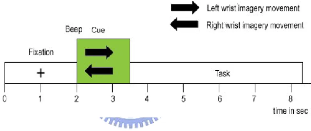
The experiment paradigm is as figure 4.1. At the beginning of each trial, a fixation cross apears on the screen indicating the subject to focus on it. The cross lasts for two seconds, after then a warning tone sounds and a left/right arrow apears on the screen, lasting for 1.5 seconds. The arrows are cues indicating the subjects to perform either a left or right wrist lifting imagery task. The subjects are told to perform the task after he/she sees the arrow disapears. Each trial ends 8 seconds after the cross apears. Because the subjects’ habit to the regularity might lead to implicit results, we apply a jittering in the paradigm to avoid so. That is, there is a randomly given 2 to 4 second interval between each trial.
There are two sessions in one experiment. In the first session, subjects are asked to perform left or right wrist lifting real movement. And in the second session, the tasks are left or right wrist lifting imagery movement. Each session goes for twenty minutes, and between two sessions there is a few minute break to avoid fatigue of the subjects. Because of the random interval between trials, the numbers of trials in each session are not always the same. But there are at least 50 trials in each task.
4.1 Offline analysis 35
Subjects
We invited five subjects in this experiment, including four males and one female, all aged 22-24. Each subject participates three to six experiments. We asked these subjects to participate one experiment about every ten days. The different number of experiment times are according to his/her performance of the results. Finally, subject A participates 5 experiments, subject B participates 3 experiments, subject C participates 5 experiments, and both subject D and subject E participate 3 experiments. In the above five, the raw data of subject E is somehow too bad to analyse. We have too few trials left after the pre-processing, so in the following results we skip the subject E. Therefore, we’ll show totally 16 experiments, including 16 real movement sessions and 16 imagery movement sessionse.
Figure 4.1: Experiment paradigm. This figure shows the experiment paradigm of wrist lifting. The time line indicates what the screen shows in every second.
Equipment setup
We prepared two computers and an 32-channel EEG cap connecting to an amplifier. The subject is asked to wear the EEG cap and sit on a comfortable chair, putting his/her hands on the table and keep them relax. There is a 17” LCD monitor set in front of the the subject, and the screen shows the visual cue described in section 4.1.1. This paradigm is controlled by computer A. The timing of each cue is sent from computer A through a parallel port to computer B, which is connected to the amplifier and records the data along with the cue points.
The data acquisition is under 1000Hz sampling rate. We start the experiment after the impedence of all 32 channels are below 3k ohm.
After an experiment is done, we use a digitizer to record the exact 3D electrode posi-tions. This information is needed as head model. We use it to calculate the forward model described in section 3.4.2 used in the MCB spatial filtering method in section 3.4.3.
Data pre-processing
After the data is recored, we apply some preprocessing:
1 EOG rejection. When the eye blinks, it brings out EOG and strongly affacts the data, especially the data recorded from the frontal channels. The detail of EOG rejection was described in section 3.2. Here we use 100 microvolt as the threshold and reject any trial that has data points exceeding this threshold.
2 Bandpass filtering. We apply a 5-30 Hz bandpass filter to the data. On one hand to avoid low frequency heartbeat artifacts, and on the other to avoid the 60 Hz power line effects and high frequency noises.
4.1.2
Data analysis
Here we show the analyses we did after the data was pre-processed.
Time-frequency analysis
First we do some basic analyses to the data. Mainly because we want to make sure the data is fine before we do any further analysis. The main analysis here is Time-Frequency analysis using morlet wavelet transform, as we described in section 3.3. We need to ob-serve some parameters to train the MCB spatial filter described in section 3.4.3, such as control/active state time period selection.
Spatial filter training
After the basic analysis we select two time periods as control state and active state. We then use this information along with the forward model to train a MCB spatial filter for
4.1 Offline analysis 37
each data. The filtered result compared to the original C4 channel data is shown in the next section. Also we analyse the filter weighting and plot it as topography map in the next chapter.
ROC curve analysis
The ROC curve analysis is used to simulate the offline data as a online recorded data. The procedure is described in section 3.5. After the training of the MCB spatial filter is done, we apply the filter to the data and compare the ROC curve between raw C4 channel data and the filtered data. From the two ROC curves we can observe the best TPR and FPR that a simple threshold can give. We then compare it to see if this scheme works.
4.1.3
Experiment results
Subject A
• Experiment 1
The TF-map is shown in figure 4.2. The filtered result compared with the C4 channel data is shown in figure 4.3.
• Experiment 2
The TF-map is shown in figure 4.4. The filtered result compared with the C4 channel data is shown in figure 4.5.
• Experiment 3
The TF-map is shown in figure 4.6. The filtered result compared with the C4 channel data is shown in figure 4.7.
• Experiment 4
The TF-map is shown in figure 4.8. The filtered result compared with the C4 channel data is shown in figure 4.9.
^ c u e
(a) real movement
^ c u e
(b) imagery movement
Figure 4.2: The Time-Frequency map of Subject A. The frequency ranges from 6 to 30 Hz, and the timeline is an eight-second trial. The visual cue indicating the motor movement is at 2 second. The left figure is the real movement session and the right figure is the imagery movement session.
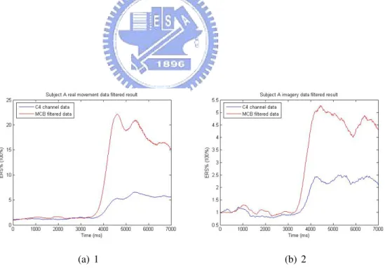
(a) real movement (b) imagery movement
Figure 4.3: The ERD/ERS curve of Experiment 1 of subject A, the visual cue appears at 2 second. The red line indicates the filtered data and the blue line indicates the original C4 data. The left figure is real movement session and the right one is imagery session
4.1 Offline analysis 39
^ c u e
(a) 1
^ c u e
(b) 2
Figure 4.4: The Time-Frequency map of Subject A. The frequency ranges from 6 to 30 Hz, and the timeline is an eight-second trial. The visual cue indicating the motor movement is at 2 second. The left figure is the real movement session and the right figure is the imagery movement session.
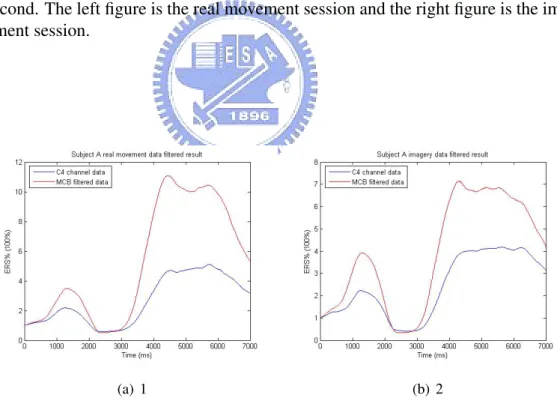
(a) 1 (b) 2
Figure 4.5: The ERD/ERS curve of Experiment 2 of subject A, the visual cue appears at 2 second. The red line indicates the filtered data and the blue line indicates the original C4 data. The left figure is real movement session and the right one is imagery session
^ c u e
(a) 1
^ c u e
(b) 2
Figure 4.6: The Time-Frequency map of Subject A. The frequency ranges from 6 to 30 Hz, and the timeline is an eight-second trial. The visual cue indicating the motor movement is at 2 second. The left figure is the real movement session and the right figure is the imagery movement session.
(a) 1 (b) 2
Figure 4.7: The ERD/ERS curve of Experiment 3 of subject A, the visual cue appears at 2 second. The red line indicates the filtered data and the blue line indicates the original C4 data. The left figure is real movement session and the right one is imagery session
4.1 Offline analysis 41
^ c u e
(a) 1
^ c u e
(b) 2
Figure 4.8: The Time-Frequency map of Subject A, Experiment 4. The left figure is the real movement session and the right figure is the imagery movement session.
(a) 1 (b) 2
Figure 4.9: The ERD/ERS curve of Experiment 4 of subject A, the visual cue appears at 2 second. The left figure is real movement session and the right one is imagery session
(a) 1 (b) 2
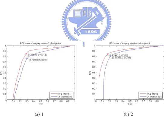
Figure 4.10: ROC curve analysis of Subject A, imagery session 1 and 2. The red line is the ROC curve of the filtered data and the blue line is the ROC curve of the C4 channel data.
(a) 1 (b) 2
Figure 4.11: ROC curve analysis of Subject A, imagery session 3 and 4. The red line is the ROC curve of the filtered data and the blue line is the ROC curve of the C4 channel data.
4.1 Offline analysis 43
subject A left wrist imagery movement
Dataset ERS% ERD% ERS%-ERD% TPR FPR
C4 channel data 181% 56% 125% 0.62 0.37 1 MCB filtered data 369% 74% 295% 0.84 0.33 C4 channel data 315% 41% 274% 0.63 0.38 2 MCB filtered data 398% 32% 366% 0.83 0.32 C4 channel data 447% 89% 358% 0.76 0.29 3 MCB filtered data 892% 78% 814% 0.84 0.28 C4 channel data 212% 81% 131% 0.80 0.21 4 MCB filtered data 408% 89% 319% 0.84 0.17 Table 4.1: Subject B • Experiment 1
The TF-map is shown in figure 4.12. The filtered result compared with the C4 chan-nel data is shown in figure 4.13.
• Experiment 2
The TF-map is shown in figure 4.14. The filtered result compared with the C4 chan-nel data is shown in figure 4.15.
• Experiment 3
The TF-map is shown in figure 4.16. The filtered result compared with the C4 chan-nel data is shown in figure 4.17.
^ c u e
(a) 1
^ c u e
(b) 2
Figure 4.12: The Time-Frequency map of Subject B. The frequency ranges from 6 to 30 Hz, and the timeline is an eight-second trial. The visual cue indicating the motor movement is at 2 second. The left figure is the real movement session and the right figure is the imagery movement session.
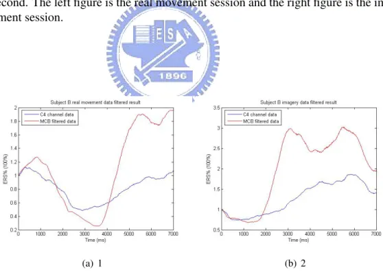
(a) 1 (b) 2
Figure 4.13: The ERD/ERS curve of Experiment 1 of subject B, the visual cue appears at 2 second. The red line indicates the filtered data and the blue line indicates the original C4 data. The left figure is real movement session and the right one is imagery session
4.1 Offline analysis 45
^ c u e
(a) 1
^ c u e
(b) 2
Figure 4.14: The Time-Frequency map of Subject B. The frequency ranges from 6 to 30 Hz, and the timeline is an eight-second trial. The visual cue indicating the motor movement is at 2 second. The left figure is the real movement session and the right figure is the imagery movement session.
(a) 1 (b) 2
Figure 4.15: The ERD/ERS curve of Experiment 2 of subject B, the visual cue appears at 2 second. The red line indicates the filtered data and the blue line indicates the original C4 data. The left figure is real movement session and the right one is imagery session
^ c u e
(a) 1
^ c u e
(b) 2
Figure 4.16: The Time-Frequency map of Subject B. The frequency ranges from 6 to 30 Hz, and the timeline is an eight-second trial. The visual cue indicating the motor movement is at 2 second. The left figure is the real movement session and the right figure is the imagery movement session.
(a) 1 (b) 2
Figure 4.17: The ERD/ERS curve of Experiment 3 of subject B, the visual cue appears at 2 second. The red line indicates the filtered data and the blue line indicates the original C4 data. The left figure is real movement session and the right one is imagery session
4.1 Offline analysis 47
Subject C
• Experiment 1
The TF-map is shown in figure 4.18. The filtered result compared with the C4 chan-nel data is shown in figure 4.19.
• Experiment 2
The TF-map is shown in figure 4.20. The filtered result compared with the C4 chan-nel data is shown in figure 4.21.
• Experiment 5
The TF-map is shown in figure 4.22. The filtered result compared with the C4 chan-nel data is shown in figure 4.23.
^ c u e
(a) 1
^ c u e
(b) 2
Figure 4.18: The Time-Frequency map of Subject C. The frequency ranges from 6 to 30 Hz, and the timeline is an eight-second trial. The visual cue indicating the motor movement is at 2 second. The left figure is the real movement session and the right figure is the imagery movement session.
(a) 1 (b) 2
Figure 4.19: The ERD/ERS curve of Experiment 1 of subject C, the visual cue appears at 2 second. The red line indicates the filtered data and the blue line indicates the original C4 data. The left figure is real movement session and the right one is imagery session
4.1 Offline analysis 49
^ c u e
(a) 1
^ c u e
(b) 2
Figure 4.20: The Time-Frequency map of Subject C. The frequency ranges from 6 to 30 Hz, and the timeline is an eight-second trial. The visual cue indicating the motor movement is at 2 second. The left figure is the real movement session and the right figure is the imagery movement session.
(a) 1 (b) 2
Figure 4.21: The ERD/ERS curve of Experiment 2 of subject C, the visual cue appears at 2 second. The red line indicates the filtered data and the blue line indicates the original C4 data. The left figure is real movement session and the right one is imagery session
^ c u e
(a) 1
^ c u e
(b) 2
Figure 4.22: The Time-Frequency map of Subject C. The frequency ranges from 6 to 30 Hz, and the timeline is an eight-second trial. The visual cue indicating the motor movement is at 2 second. The left figure is the real movement session and the right figure is the imagery movement session.
(a) 1 (b) 2
Figure 4.23: The ERD/ERS curve of Experiment 5 of subject C, the visual cue appears at 2 second. The red line indicates the filtered data and the blue line indicates the original C4 data. The left figure is real movement session and the right one is imagery session
4.1 Offline analysis 51
Subject D
• Experiment 1
The TF-map is shown in figure 4.24. The filtered result compared with the C4 chan-nel data is shown in figure 4.25.
• Experiment 2
The TF-map is shown in figure 4.26. The filtered result compared with the C4 chan-nel data is shown in figure 4.27.
^ c u e
(a) 1
^ c u e
(b) 2
Figure 4.24: The Time-Frequency map of Subject D. The frequency ranges from 6 to 30 Hz, and the timeline is an eight-second trial. The visual cue indicating the motor movement is at 2 second. The left figure is the real movement session and the right figure is the imagery movement session.
(a) 1 (b) 2
Figure 4.25: The ERD/ERS curve of Experiment 1 of subject D, the visual cue appears at 2 second. The red line indicates the filtered data and the blue line indicates the original C4 data. The left figure is real movement session and the right one is imagery session
4.1 Offline analysis 53
^ c u e
(a) 1
^ c u e
(b) 2
Figure 4.26: The Time-Frequency map of Subject D. The frequency ranges from 6 to 30 Hz, and the timeline is an eight-second trial. The visual cue indicating the motor movement is at 2 second. The left figure is the real movement session and the right figure is the imagery movement session.
(a) 1 (b) 2
Figure 4.27: The ERD/ERS curve of Experiment 2 of subject D, the visual cue appears at 2 second. The red line indicates the filtered data and the blue line indicates the original C4 data. The left figure is real movement session and the right one is imagery session
4.2
Online feedback experiment
In this chapter we show the experiment results of online feedback experiments. First we introduce the experiment setup, including information about session time, trial time, experiment paradigm, data pre-processing, and online processing scheme. Then we show the results of online feedback experiments compared with the offline experiment results. In the end of this chapter we give a brief discussion about our experiment and the results.
4.2.1
Experiment setup
Figure 4.28: Online experiment paradigm design. This figure shows the experiment paradigm of online experiment of wrist imagery movement. The time line indicates what the screen shows in every second. The visual cue appears at 2 second and lasts for 1.5 second. The visual feedback starts at 4.5 second and ends at 8 second.
Figure 4.29: Online experiment visual feedback. The visual feedback is a expanding-contracting bar, indicating the ERS% at the moment.
4.2 Online feedback experiment 55
Experiment paradigm
The online feedback experiment paradigm is pretty much like the offline one. As fig-ure 4.28 shows, a fixation cross appears in the center of the screen at the beginning of a trial. The cross lasts for 2 seconds and a warning tone sounds, followed with an arrow appearing on the screen, indicating the subject to perform a left wrist imagery movement or to keep resting. The arrow lasts for 3 seconds and a visual feedback starts on the screen. The visual feedback is like figure 4.29. It’s a bar extending or contracting as the power changes.
In each experiment, we have two sessions. The first session is just like an offline exper-iment session described in section 4.1.1. Then we use the data recorded in this session to train a MCB spatial filter, and we apply this spatial filter to online filter the the data in the second session. The second session will give the subjects a visual feedback on the screen according to the online filtered results.
Subjects
In the online feedback session, we test only one subject. We pick subject A, the one who gets significant results in the offline experiments. We can say he’s a well-trained subject. This subject participates 2 online feedback experiments, with a few days interval between them.
Data processing
In the first session we do the data processing just like we described in the previous chapter. As for the second online feedback session, the data is recorded in 1000Hz sampling rate and is online filtered by an 8-12Hz bandpass filter. We then online apply the spatial filter trained in the first session to the second session.
Feedback