低空探空火箭的氣動力性質模擬

(1)

國立交通大學

機械工程學系

碩士論文

Simulation of Aerodynamics Properties of

a Low-Altitude Sounding Rocket

低空探空火箭的氣動力性質模擬

研究生：古必任

指導教授：吳宗信博士

(2)

低空探空火箭的氣動力性質模擬

Simulation of Aerodynamics Properties of

a Low-Altitude Sounding Rocket

研究生：古必任

Student：Bi-Ren Gu

指導教授：吳宗信博士

Advisor：Dr. Jong-Shinn Wu

國立交通大學

機械工程學系

碩士論文

A Thesis

Submitted to Department of Mechanical Engineering

College of Engineering

National Chiao Tung University

in Partial Fulfillment of the Requirements

for the Degree of

Master of Science

In

Mechanical Engineering

July 2009

Hisnchu, Taiwan

西元 2009 年 7 月

(3)

低空探空火箭的氣動力參數模擬

學生：古必任

指導教授：吳宗信博士

國立交通大學機械工程學系

摘要

探空火箭(sounding rocket)是太空運載工具的一種，採取省去

導引及控制系統來降低成本，利用機翼或裙狀外型來進行氣動力控

制，保持火箭穩定飛行。探空火箭主要功能為運送精密探測儀器進入

地球軌道進行自然現象的探測行為。探空火箭飛行在不同的階段：在

不同速度情況下有次音速、穿音速、超音速到極超音速等階段；大氣

密度也隨著不斷攀升的高度而變動，此時火箭會經歷連續流場、過度

流場以及稀薄氣體流場。在探空火箭的氣動以及熱傳系統設計領域

中，各具特色的飛行環境的所造成不同的氣動及熱傳模擬方法的建構

是非常重要的。UNIC-UNS 是一套求解 Navier-Stokes 方程式的程式，

在這份研究當中，我們利用這個程式來模擬探空火箭在不同飛行階段

與各具特色的大氣環境中，氣動及熱傳情況。我們首先必須做網格測

試來選擇最有效率的網格數量，再利用此網格來進行不同飛行階段：

不同的馬赫數、大氣密度以及飛行攻角的氣動力性質模擬。最後再比

(4)

較層流模組跟紊流模組模擬出來的結果。由結果可以看出，當雷諾數

小於 10

5

時，使用層流模組模擬出來的結果較準，當雷諾數大於 10

6

時，使用紊流模組模擬出來的結果較準，而雷諾數介於這兩者中間的

流場條件，則視為過度區，用此兩種流場型態去模擬都不能夠得到非

常準確的結果。

(5)

Simulation of Aerodynamics Properties of

a Low-Altitude Sounding Rocket

Student: Bi-Ren Gu

Advisor: Dr. Jong-Shinn Wu

Department of Mechanical Engineering

National Chiao-Tung University

Abstract

Sounding rocket is one kind of launch vehicles. It uses aerodynamic self-control to keep the stability of the rocket in the period of flying. A sounding rocket is used to carry a payload into the orbit or out Earth’s gravity entirely. The sounding rocket flies through different velocities, such as subsonic, sonic, supersonic and hypersonic. Atmospheric density varies with the height, so the sounding rocket flies over the continuous flow, transitional flow and rare flow. To the aerodynamics force and heat transfer design systems of the sounding rocket, it is very important to overcome the aerodynamics and heat transfer problems caused by different kinds of flight environment. In this study, we apply a parallelized Navier-Stokes equation solver,

(6)

named UNIC-UNS, to simulate aerodynamics and heat transfer condition of sounding rocket at different stages of flight. We make the grid convergence test first to choose the most efficient grids. We simulate aerodynamics with different stages, Mach numbers, atmospheric densities and attack angles. 2. When Re<105_{, and Re>10}6_,

we can use laminar and turbulent flow model respectively. When 105_<Re<106_{, we can}

(7)

誌謝

本篇論文能夠完成，首先要感謝指導老師吳宗信教授的指導，在研究

上，幫我指引出研究的方向，使我有目標可以追求，並且教導我做人

做事該有的方法及態度。另外要感謝黃俊誠老師以及陳彥升博士，感

謝他們在忙碌之餘仍抽空幫我解決研究上的疑難雜症。感謝洪捷粲、

邱沅明、柳志良、蘇正勤、鄭凱文、林昆模、李允民、吳玟琪、胡孟

樺、林雅茹、林宗漢、江明鴻、劉育宗、鄭承志、曾坤璋、連又永等

諸位學長姐，感謝他們在研究及生活上的關心及照顧。感謝穎志、逸

民、俊傑、振庭等同學兩年來學業及生活上的相互扶持。感謝子豪、

皓遠、其璋、瑞祥、柏村、冠融等學弟的幫忙及協助。最後要感謝在

我所有的家人們以及佳芳在我求學階段中給予我的支持，讓我在學業

上無後顧之憂，專心於研究。

必任謹致

于新竹交大

2009 年 8 月

(8)

List of Tables

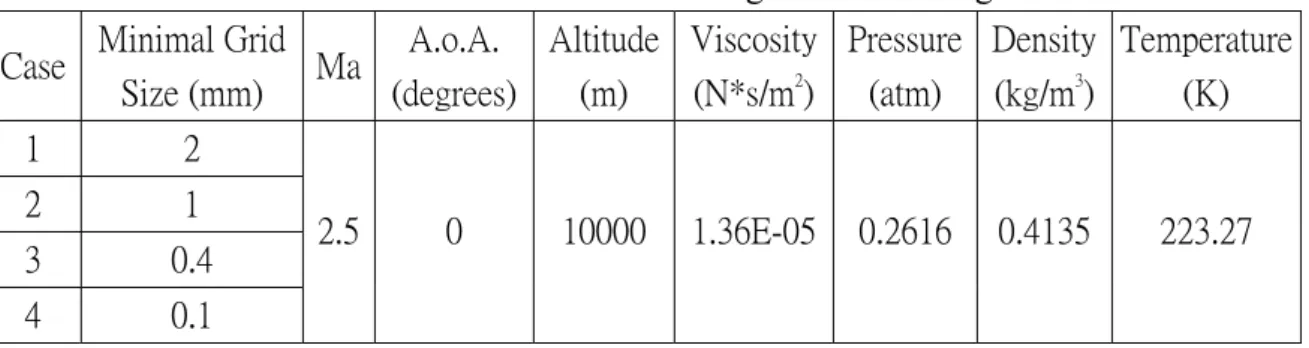
Table 1 Flow conditions of minimum grid size convergence test...25

Table 2 Simulation conditions of minimum grid size convergence test...25

Table 3 The results of minimum grid size convergence test...25

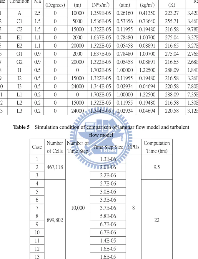
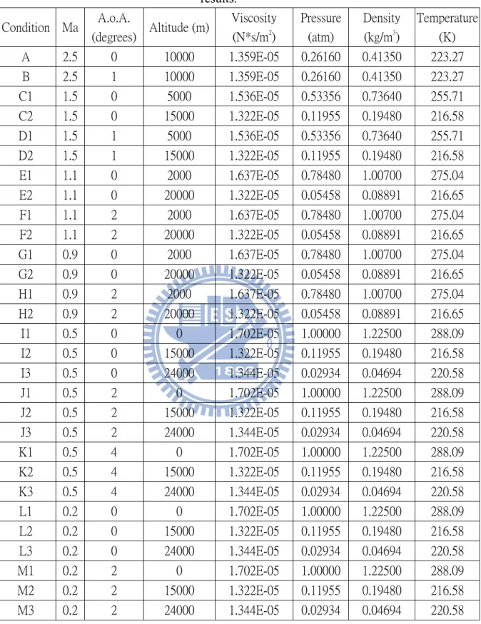
Table 4 Flow conditions of comparison of laminar model and turbulent model...26

Table 5 Simulation condition of comparison of laminar flow model and turbulent flow model.26 Table 6 Flow conditions of simulation choose from 3DOF trajectory simulation results. ...27

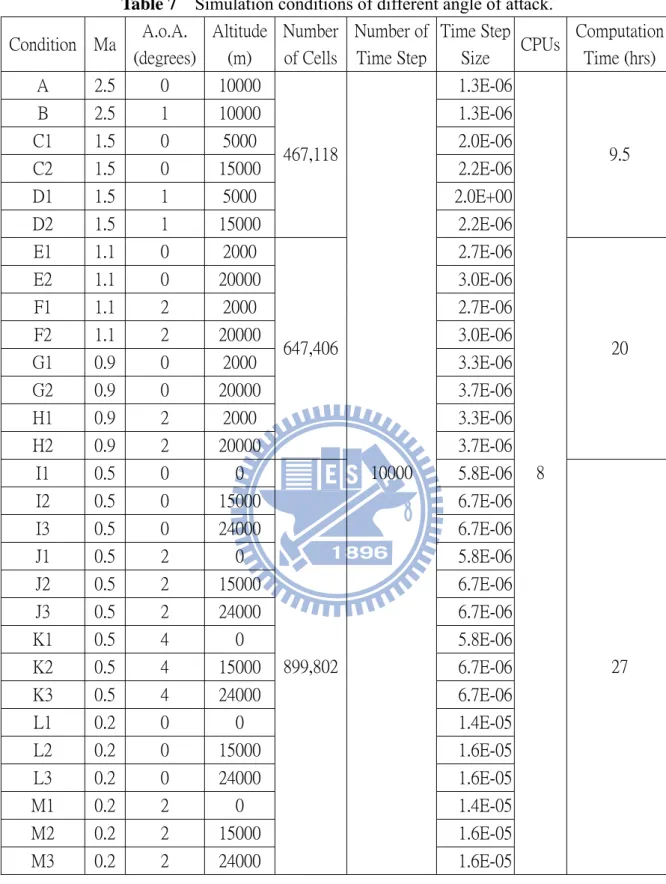
Table 7 Simulation conditions of different angle of attack...28

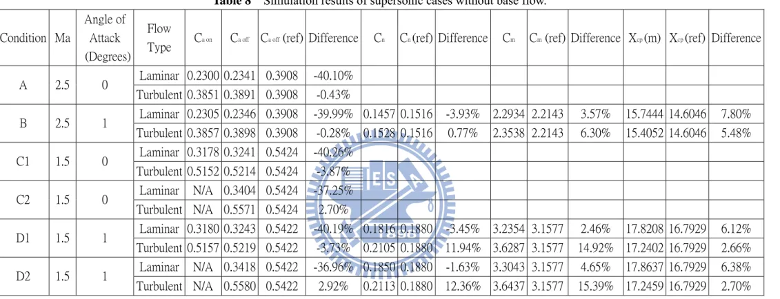
Table 8 Simulation results of supersonic cases without base flow. ...29

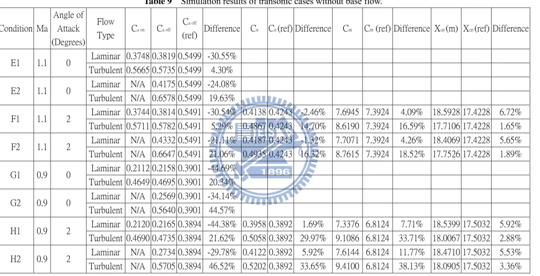
Table 9 Simulation results of transonic cases without base flow...30

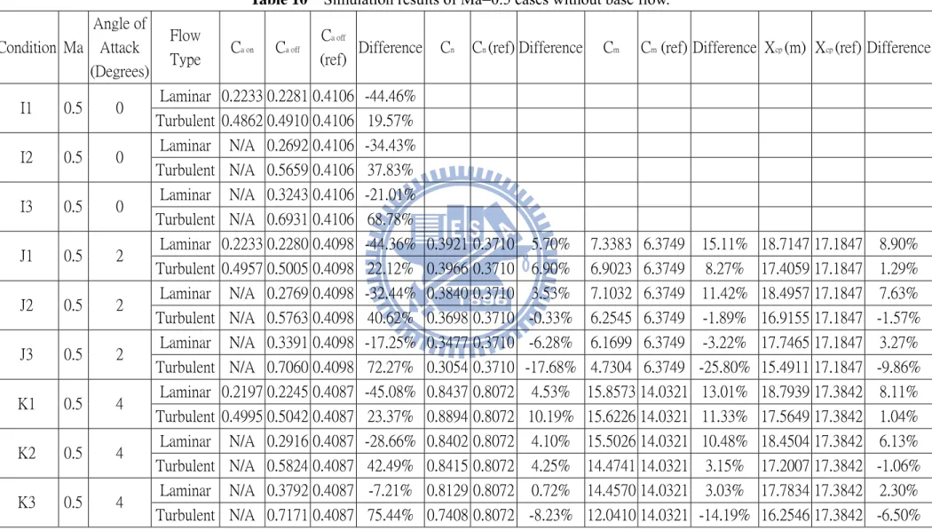
Table 10 Simulation results of Ma=0.5 cases without base flow...31

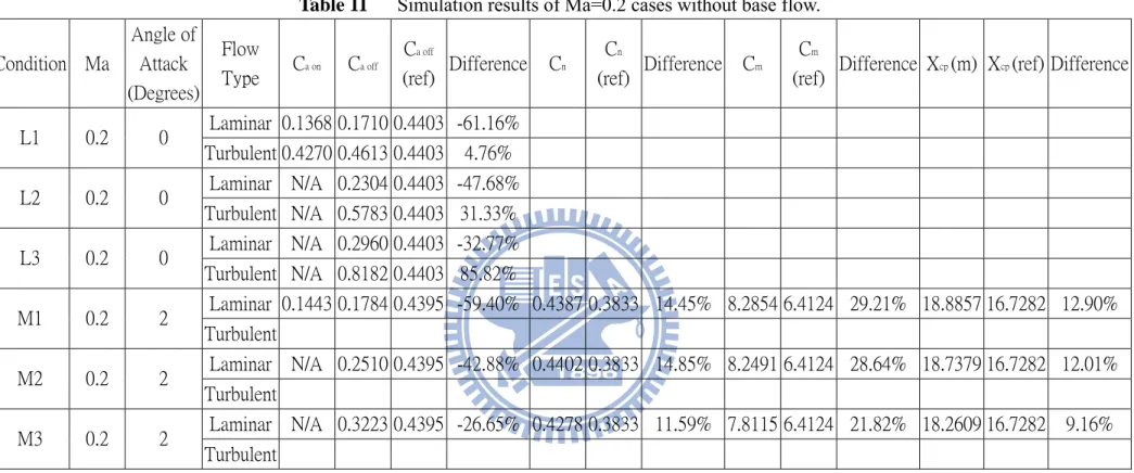
Table 11 Simulation results of Ma=0.2 cases without base flow...32

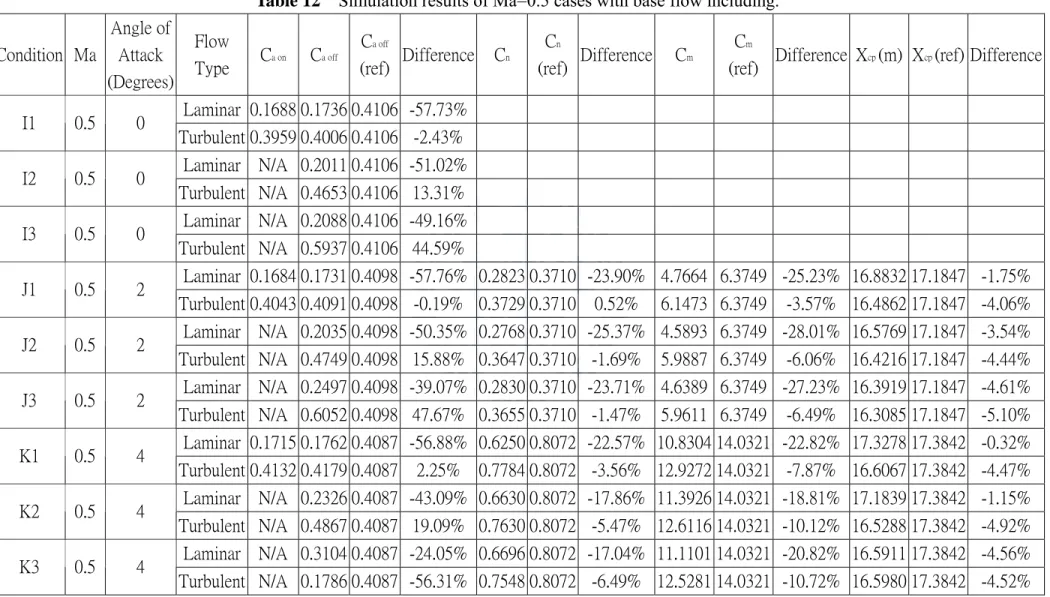
Table 12 Simulation results of Ma=0.5 cases with base flow including. ...33

(11)

List of Figures

Figure 1.1 The flying diagram of Formosat-2 ...35

Figure 1.2 Generic supersonic transport configuration SYN87-MB Grid Structure: 180 Blocks ...36

Figure 1.3 Generic supersonic transport configuration SYN87-MB solution pressure coefficient (Mach=2.2 α =3.150 C_L =0.105)...36

Figure 1.4 Satellite launch vehicle configuration. ...37

Figure 1.5 Transonic flow over the satellite launch vehicle...38

Figure 1.6 NAL jet-powered experimental airplane with a small rocket booster...38

Figure 1.7 Unstructure mesh generated around the experimental airplane...38

Figure 1.8 Computed pressure contours of the airplane and booster and enlarged views around the intake with and without a small booster: (A) and (C)M_∞ =1.4, α =5.0; and (B) and (D) M_∞ =1.7, α =4.9. ...39

Figure 2.1 Unstructured control volume...40

Figure 3.1 The Results of 3DOF trajectory simulation. ...40

Figure 3.2 Sounding rocket configuration. ...40

Figure 3.3 Typical grid distribution of aerodynamics simulation of sounding rocket. (A) grid distribution of symmetric plane, (B) grid distribution of external flow field, (C) grid distribution of body surface, (D) grid distribution of fin surface. ...42

Figure 3.4 The comparison of minimum grid size: (A)Δx_min =2mm, (B)Δx_min =1mm, (C)Δx_min =0.4mm, (D)Δx_min =0.1mm...44

Figure 3.5 Aerodynamics simulation results of laminar flow model and turbulent model, (A) case 1, (B) case 2, (C) case 3, (D) case 4, (E) case 5, (F) case 6, (G) case 7, (H) case 8, (I) case 9, (J) case 10, (K) case 11, (L) case 12, (M) case 13...46

Figure 3.6 Difference of axial-force coefficients between numerical results and reference data, (A) supersonic cases, case 1~3, (B) transonic cases, case 4~7, (C) subsonic cases, case 8~13. ...48

Figure 3.7 Difference of axial-force coefficient between numerical results and reference data..49

Figure 3.8 The density, pressure and Mach number distributions at Ma=2.5, A.o.A.=0 degree, H=10000 m...50

Figure 3.9 The density, pressure and Mach number distributions at Ma=2.5, A.o.A.=1 degree, H=10000 m...50 Figure 3.10 The density, pressure and Mach number distributions at Ma=1.5, A.o.A.=0 degree,

(12)

H=5000 m...51 Figure 3.11 The density, pressure and Mach number distributions at Ma=1.5, A.o.A.=0 degree,

(13)

Nomenclature

a C ： axial-foecr coefficient m C ： pitching-moment coefficient n C ： normal-force coefficient α n

C ： normal-force curve slope L ： model length l ： diameter of cylinder M ： Mach number P ： pressure 0 P ： stagnation pressure b P ： base pressure ∞

P ： pressure of freestream far field q _{： heat flux}

0

q ： stagnation heat flux

Re ： Reynolds number S ： area of cross section T ： temperature

∞

T ： temperature of freestream far field V ： velocity

∞

V ： velocity of freestream far field CP

X ： center of pressure location α ： angle of attack

X

Δ ： character length of HB-2 model μ _{： viscosity}

ρ _{： density}

∞

ρ ： density of freestream far field φ ： angle of roll

Subscripts

0 ： stagnation

(14)

Chapter 1 Introduction

1.1 Background and Motivation

1.1.1 Importance of Sounding Rocketry

A sounding rocket used to carry a payload to fly against the Earth’s gravity and finally into the orbit or outer space. In recent years, the rocket development has become a focus of many countries’ attention. The rocket design is one kind of the conformity technologies that contains much knowledge. It has contained the aerodynamics, heat transfer, structure analysis, control system, propulsion system and so forth.

1.1.2 Importance of Aerodynamics

In the design process, one but had decided the mission and the rocket flight path, then have often decided the majority of designs like the rocket size, propelling power and etc. We may see Figure 1.1, the rocket flies through various stages such as subsonic, sonic, supersonic, and hypersonic. Atmospheric density varies with the height, so the rocket flies over the continuous flow, transitional flow and rare flow. The rocket under the different speeds, the different air densities and the different

(15)

aerodynamics forces influences all needs to go overcomes when designing the rocket. And now, we want to introduce some important aerodynamics coefficients in this thesis.

1.1.2.1 Axial-Force Coefficient

The axial-force coefficient, C , is defined as, _a

S V F C a a ₂ 2 1 ∞ ∞ = ρ

Where F is axial-force acting on the reverse direction with the direction of the _a rocket to fly, ρ is density of far-field freestream, _∞ V_∞ is velocity of far-field freestream, S is the cross section area. The higher the C is, the more thrust the _a rocket needs to fly. And then, we want to introduce two kinds of the axial-force coefficients, on-burning axial-force coefficient and off-burned axial-force coefficient.

The is axial-force acting when the thrust is pushing the rocket, and the . is axial-force acting when the thrust turn off.

1.1.2.2 Normal-Force Coefficient

The normal-force coefficient, C , is defined as, _n

S V F C n n ₂ 2 1 ∞ ∞ = ρ S V F Caon aonburning₂ 2 1 ∞ ∞ − = ρ S V F

C_a_off aoff burned₂

2 1 ∞ ∞ − = ρ burning on a F ₋ burned off a F ₋

(16)

Where F is normal-force, _n ρ_∞ is density of far-field freestream, V_∞ is velocity of far-field freestream, S is the cross section area.

1.1.2.3 Pitching-Moment Coefficient

The normal-force coefficient, C , is defined as, _m

Sl V M C_m p₂ 2 1 ∞ ∞ = ρ

Where M is pitching-moment, p ρ∞ is density of far-field freestream, V∞ is velocity of far-field freestream, S is the cross section area, l is the diameter of cylinder.

1.1.2.4 Pressure Center

The pressure center, Xcp, is defined as,

n m cp C C X =

We set the top of nose of the sounding rocket as the original point to calculate the

cp X .

(17)

1.2 Literatures Survey

Because of the progressing of the computational ability of computer, aerodynamics and heat transfer simulations are applied to many applications, such as building construction, cars, airplanes, rockets and so forth.

In 1999 J. Reuther [J. Reuther, 1999] did the application of a control theory-based aerodynamic shape optimization method did the problem of supersonic aircraft design. A high fidelity computational fluid dynamics algorithm modeling the Euler equation is used to calculate the aerodynamic properties of complex three-dimensional aircraft configurations, see Figure 1.2 and Figure 1.3.

In 2001, Paulo Moraes Jr. [Paulo Moraes Jr., 2001] did the wind tunnel testing. The tests were carried out in high speed continuous and blow-down wind tunnels using 1/15th_{and 1/30}th_{scale satellite launch vehicle models of the complete configuration,} Figure 1.4. Through this experimental investigation in high speed wind tunnels, they

can understand the flow behavior very well, Figure 1.5.

In 2005, Fumiya Togashi and et al. [Fumiya Togashi et al., 2005] used overset unstructured grids to simulate supersonic airplane/booster separation, see Figure 1.6 and Figure 1.7. An unstructured grid around the rocket booster is overset on the stationary grid around the airplane and moves with time to simulate the separation process. They solved the Euler equations for compressible inviscid flows. The

(18)

numbers of cells is about four million. Some results are shown in Figure 1.8.

1.3 Specific Objectives of the Thesis

By using the 3DOF trajectory simulation [Matthew Ross Smith], we make a table of flow conditions that we want to know the details of aerodynamics properties. Then, we do the minimum grid size convergence test of the sounding rocket to choose the most efficient mesh file with UNIC-UNS code [Chen, Y.S.]. And then, we use the mesh file to do the aerodynamics simulation with laminar flow model and turbulent flow model and to compare which one of the two models is more close to the physical phenomenon. Then, we simulate aerodynamics properties with all the flow conditions of the flight trajectory and discuss the physical meaning of the results.

(19)

Chapter 2 Numerical Method

In this proposal, we use the UNIC-UNS code, developed by Y.S. Chen et al, to simulate an unsteady compressible flow. It uses Navier-Stokes solver with finite volume method. The governing equation, boundary condition, numerical methods, algorithm and so on will be discussed below.

2.1 Governing Equations

The general form of mass conservation, energy conservation, Navier-Stokes equation and other transport equations can be written in Cartesian tensor form:

( )

₍

₎

φ φ φ μ φ ρ ρφ S x x U x t j j j j + ⎟ ⎟ ⎠ ⎞ ⎜ ⎜ ⎝ ⎛ ∂ ∂ ∂ ∂ = ∂ ∂ + ∂ ∂ (1) where μφ_{is an effective diffusion coefficient,}S denotes the source term, φ ρ

is the fluid density and φ= (1, u, v, w, h, k,ε ) stands for the variables for the mass, momentum, total energy and turbulence equation, respectively.

2.2 Spatial Discretization

The cell-centered scheme is employed here then the control volume surface can be represented by the cell surfaces and the coding structure can be much simplified. The transport equations can also be written in integral form as:

(20)

∫

Ω Γ Ω Ω Ω = Γ ⋅ + Ω ∂ ∂ d S d n F d t r r ρφ (2)

where Ω is the domain of interest, Γ the surrounding surface, nr_{the unit} normal in outward direction. The flux function Fr consists of the inviscid and the viscous parts: φ μ φ ρ − _φ∇ = V Fr v (3)

The finite volume formulation of flux integral can be evaluated by the summation of the flux vectors over each face,

( )

∫

∑

Γ = ΔΓ = Γ ⋅ i k j j j i F d n Fr r _, (4)

where k(i) is a list of faces of cell i, Fi,j represents convection and diffusion fluxes through the interface between cell i and j, ΔΓj is the cell-face area.

The viscous flux for the face e between control volumes P and E as shown in

Figure 2.1 can be approximated as:

(

)

_⎟⎟ ⎠ ⎞ ⎜ ⎜ ⎝ ⎛ − − − ⋅ ∇ + − − ≈ ⋅ ∇ r r r r n r r n E P E e P E P E e r r r r r r r r φ φ _φ φ (5) That is based on the consideration that

(

E P

)

e P E r r r r − ⋅ ∇ ≈ −φ φ φ ₍₆₎

where ∇ is interpolated from the neighbor cells E and P. φ

The inviscid flux is evaluated through the values at the upwind cell and a linear reconstruction procedure to achieve second order accuracy

(21)

(

e u

)

u e u e r r r r − ⋅ ∇ Ψ + =φ φ φ ₍₇₎

where the subscript u represents the upwind cell and Ψe is a flux limiter used to prevent from local extrema introduced by the data reconstruction. The flux limiter proposed by Barth [Barth, T.J., 1993] is employed in this work. Defining

(

φu φj

)

φ

(

φu φj

)

φ_max =max , , _min =min , _{, the scalar}Ψ_e_{associated with the gradient at} cell u due to edge e is

⎪ ⎪ ⎪ ⎩ ⎪ ⎪ ⎪ ⎨ ⎧ < − ⎟⎟ ⎠ ⎞ ⎜⎜ ⎝ ⎛ − − > − ⎟⎟ ⎠ ⎞ ⎜⎜ ⎝ ⎛ − − = Ψ 1 0 , 1 min 0 , 1 min 0 0 min 0 0 max φ φ φ φ φ φ φ φ φ φ φ φ e u e u e u e u e if if (8)

where φe0 is computed without the limiting condition (i.e. Ψe=1)

2.3 Time Integration

A general implicit discretized time-marching scheme for the transport equations can be written as:

(

)

φ ρφ φ φ ρ S t A A t n P n m NB m m n P P n + Δ + = ⎟⎟ ⎠ ⎞ ⎜⎜ ⎝ ⎛ + Δ + = +

∑

1 1 1 (9)

where NB means the neighbor cells of cell P. The high order differencing terms and cross diffusion terms are treated using known quantities and retained in the source term and updated explicitly.

(22)

φ φ φ ρ SU A A t m NB m m P P n + Δ = Δ ⎟⎟ ⎠ ⎞ ⎜⎜ ⎝ ⎛ + Δ

∑

=1 ₍₁₀₎ θ φ φ φ φ ⎟ ⎠ ⎞ ⎜ ⎝ ⎛ ₊ _Δ ₋ =

∑

= n P n m NB m m A A S SU 1 (11)

where θ is a time-marching control parameter which needs to specify. θ = 1 and θ = 0.5 are for implicit first-order Euler time-marching and second-order time-centered time-marching schemes. The above derivation is good for non-reacting flows. For general applications, a dual-time sub-iteration method is now used in UNIC-UNS for time-accurate time-marching computations.

2.4 Pressure-Velocity-Density Coupling

In an extended SIMPLE [Chen, Y.S., 1989] family pressure-correction algorithm, the pressure correction equation for all-speed flow is formulated using the perturbed equation of state, momentum and continuity equations. The simplified formulation can be written as:

p p p u u u p D u RT n n n n u∇ ′ = + ′ = + ′ − = ′ ′ = ′ _;r _;r +1 r r_; +1 γ ρ ρ (12)

( ) ( )

( )

n n u t u u t r r r_ρ _ρ ρ _ρ ρ ₋_∇ ⎟ ⎠ ⎞ ⎜ ⎝ ⎛ ∂ ∂ − = ′ ∇ + ′ ∇ + ∂ ′ ∂ (13)

where Du is the pressure-velocity coupling coefficient. Substituting Eq. (12) into Eq. (13), the following all-speed pressure-correction equation is obtained,

(

)

( )

n n u p D p _ρ ρ _ρr γ ⎟ −∇⋅ ⎞ ⎜ ⎛Δ ′ − = ′ ∇ ⋅ ∇ + ′ ⋅ 1

(23)

For the cell-centered scheme, the flux integration is conducted along each face and its contribution is sent to the two cells on either side of the interface. Once the integration loop is performed along the face index, the discretization of the governing equations is completed. First, the momentum equation (9) is solved implicitly at the predictor step. Once the solution of pressure-correction equation (14) is obtained, the velocity, pressure and density fields are updated using Eq. (12). The entire corrector step is repeated 2 and 3 times so that the mass conservation is enforced. The scalar equations such as turbulence transport equations, species equations etc. are then solved sequentially. Then, the solution procedure marches to the next time level for transient calculations or global iteration for steady-state calculations. Unlike for incompressible flow, the pressure-correction equation, which contains both convective and diffusive terms is essentially transport-like. All treatments for inviscid and the viscous fluxes described above are applied to the corresponding parts in Eq. (14).

2.5 Linear Matrix Solver

The discretized finite-volume equations can be represented by a set of linear algebra equations, which are non-symmetric matrix system with arbitrary sparsity patterns. Due to the diagonal dominant for the matrixes of the transport equations, they can converge even through the classical iterative methods. However, the

(24)

coefficient matrix for the pressure-correction equation may be ill conditioned and the classical iterative methods may break down or converge slowly. Because satisfaction of the continuity equation is of crucial importance to guarantee the overall convergence, most of the computing time in fluid flow calculation is spent on solving the pressure-correction equation by which the continuity-satisfying flow field is enforced. Therefore the preconditioned Bi-CGSTAB [Van Der Vorst, H.A., 1992] and GMRES [Saad, Y. and Schultz, M.H., 1986] matrix solvers are used to efficiently solve, respectively, transports equation and pressure-correction equation.

2.6 Parallelization

Compared with a structured grid approach, the unstructured grid algorithm is more memory and CPU intensive because “links” between nodes, faces, cells, needs to be established explicitly, and many efficient solution methods developed for structured grids such as approximate factorization, line relaxation, SIS, etc. cannot be used for unstructured methods.

As a result, numerical simulation of three-dimensional flow fields remains very expensive even with today’s high-speed computers. As it is becoming more and more difficult to increase the speed and storage of conventional supercomputers, a parallel architecture wherein many processors are put together to work on the same problem

(25)

unlimited. It is reasonable to claim that parallel computing can provide the ultimate throughput for large-scale scientific and engineering applications. It has been demonstrated that performance that rivals or even surpasses supercomputers can be achieved on parallel computers.

(26)

Chapter 3 Results and Discussion

3.1 Overview

In this thesis, we use the UNIC-UNS code to simulate the surface properties of the sounding rocket. These surface properties include drag force, normal force, pitching moment and pressure center. In order to simulate these properties accurately and quickly, we should do minimum grid size convergence test. Then, we use the grid to do the aerodynamics simulation with laminar flow model and turbulent flow model, see Table 1 and Table 2, and to compare which one of the two models is more close to the physical phenomenon. This is very important of the near-wall flow field. Then, we simulate aerodynamics properties with all the flow conditions of the flight trajectory, see Figure 3.1 and Table 6, and discuss the physical meaning of the results.

3.2 Grid Convergence Test

3.2.1 Grid Configuration

Figure 3.2 shows the grid configuration. The length of the sounding rocket is 350

(27)

boundary layer near the body surface. Therefore, the finer grid developed at which as the previous described. Relatively, the coarser grid is used at the inlet freestream far-field to reduce the computational cost. The grid distribution of the sounding rocket is shown in Figure 3.3. When the velocity larger than speed of sound, it is not necessary to simulate the downstream flow field because the downstream flow field do not influence the upstream flow field, so that the grids for supersonic and transonic cases do not include the base flow. It is important to save the cost of simulation. On the other hand, the girds for subsonic cases should include the base flow and extend the length of the radial, upstream and downstream external flow direction.

3.2.2 Minimum Grid Size Convergence Test

According to the dimensionless number,

x V t CFL Δ Δ

= * , the minimum grid size(Δx_{) will affect the computational time and the accuracy of the simulation. We} usually set the CFL equal to 1, and we can find when we have smaller minimum grid size, we have smaller time step size(Δt_{) with the same flow condition. It means that} we have to spend more computational time to simulate this case. Seeing the results of minimum grid size convergence test, shown in Table 2 and Table 3, we can observe that the axial-force coefficient difference with the reference axial-force coefficient in case 2 and 3 are better than case 1 and case 4. We compare the case 2 and 3, we can find the computational time in case 2 is much less than case 3. Considering the time

(28)

cost and the accuracy, we choose 1 mm to be the minimum grid size to do the further simulations.

3.3 Comparison of Laminar Flow and Turbulent Flow

In general case of external flow over a plate, we usually take Reynolds number equal to 500,000 as the critical number for laminar flow transition to turbulent flow, we define it as Re but it is a rough estimation in our case. We have to choose one _cr of laminar flow and turbulent flow as the whole flow field type to do the numerical simulation.

3.3.1 Flow Conditions and Simulation Conditions

Table 4 shows the flow conditions including Mach number, Reynolds number,

angle of attack, temperature, pressure, density and viscosity in each case. Because of the definition of Reynolds number,

μ ρVD =

Re , we can choose difference Mach numbers and altitudes to determine the see the magnitude of Reynolds number. And then, we simulate these cases in whole laminar flow field and whole turbulent flow field to see which of the flow field models is more close to our reference data. Table

5 shows the simulation conditions including the number of cells, number of time steps,

(29)

3.3.2 Results in Comparison of Laminar Flow and Turbulent Flow

Figure 3.5 shows the simulation results of axial-force. We can observe that

axial-forces acting on the rocket in turbulent flow field are larger than laminar flow field. The reason is that in turbulent flow, the momentum transfer in the boundary layer near the surface of rocket is faster than in laminar flow so that the shear stress is larger in the turbulent flow, and the axial-force is also larger. Figure 3.6 shows the difference of axial-force between numerical results and the reference data. In the supersonic cases, i.e. case 1 to 3, the Reynolds numbers are much larger than the critical Reynolds number, Re . The difference of axial-force coefficients between _cr the turbulent flow model and the reference data are less than 5%, but the difference of axial-force between the laminar flow model and the reference data are all about 40%. In the transonic cases, i.e. case 4 to 7, the Reynolds numbers of case 4 and 6 are larger than the Re , and the difference of axial-force coefficients between the _cr turbulent flow model and the reference data are better than another, respectively. The Reynolds numbers of case 5 and 7 are a little less than the Re , and the difference of _cr two flow model are almost the same, furthermore the difference of laminar flow model is better than the difference of turbulent flow model. In subsonic cases, i.e. case 8 to 13, the Reynolds number of case 8 is larger than the Re , and the _cr difference of turbulent flow model is better than another. In case 9, the Reynolds

(30)

number is a little less than the Re , but the difference of turbulent flow model still _cr better than another. In case 10 to 13, the Reynolds number s are less than the Re , _cr and the difference of both model are almost the same. Now, we can make a remark as following. When the Reynolds number is larger than the Re 1 more order, for _cr example, case 1 to 4, 6 and 8, we can use turbulent flow model to simulate the surface properties. When the Reynolds number is close to or less than the Re , for example, _cr subsonic cases, the flow type might be laminar transition to turbulent flow, so we have to discuss the results of the two flow model. Seeing Figure 3.7, when Re<105_,

the difference of axial-force coefficient between reference data and laminar flow model is more accurate than turbulent flow model. When Re>106_{, the difference of}

axial-force coefficient between reference data and turbulent flow model is more accurate than laminar flow model. When 105_<Re<106_{, the numerical axial-force}

coefficients are far from the reference data, so we can consider it as the transitional regime.

3.4 Aerodynamics Simulation with Different Angle of Attack

3.4.1 Flow Conditions and Simulation Conditions

Table 6 is the flow conditions choosing from the 3DOF simulation results, Figure

(31)

direction is not so big, comparing with the force resulting from the side wind. We have to simulate larger angle of attack in the subsonic cases. When the rocket is stably flying with super sonic speed, we could just simulate the small angle of attack. In cases of Ma=0.2, we simulate cases of A. Ao. .=0°,2°. In cases of Ma=0.5, we simulate cases of A. Ao. .=0°,2°,4°. In transonic cases of Ma=0.9 and 1.1, we simulate two angle of attack, A. Ao. .=0°,2°. In supersonic cases of Ma=1.5 and 2.5, we simulate angle of attack, A. Ao. .=0°,1°.

3.4.2 Results in Difference Angle of Attack

3.4.2.1 Density, Pressure and Mach Number Distributions

The density, pressure and Mach number distributions are shown in Figure 3.8 to

Figure 3.21. First, we can easily observe the shock wave in cases of Ma=2.5 and 1.5.

In cases of A.o.A.=0 degree, the density, pressure and Mach number distributions near the rocket surface are axial symmetry. In cases with A.o.A. equal to 1, 2 and 4 degrees, there are higher density, pressure and lower velocity in the windward side of wall than the leeward of wall.

3.4.2.2 Axial-Force Coefficients

We can observe that there are small differences between difference attack angles because the cases with less attack angle have less effect on axial-force. In supersonic

(32)

cases, the difference between the axial-force coefficients using turbulent flow model and the reference axial-force coefficients are less than 3%, this can be use to validate our numerical code. The numerical results with difference angle of attack have not large difference because our angle of attack is small. As the attack angles become large, the axial-force coefficients become larger but not a big mount. In transonic cases, the difference between the axial-force coefficients using turbulent flow model and the reference axial-force coefficients are in the range of 0% to 50%. The transonic flow is hard to predict so the difference is acceptable. In the cases of Ma=0.5, H=0 and 5000 meter, the difference between the axial-force coefficients using turbulent flow model and the reference axial-force coefficients are less than 20%. As the attack angles become large, the axial-force coefficients become larger, too. In the cases of Ma=0.2, H=24000 meter, the difference is much bigger the others because the Reynolds number of this cases are less than Re , but the difference _cr using laminar flow model is still mot small, and so as the cases of Ma=0.2. I think it could have something wrong with my setting to simulate these cases.

3.4.2.3 Normal-Force Coefficients

The sounding rocket is plane symmetry. If the angle of attack of flow field is zero, the normal-force acting on the body surface should be zero. In the case of Ma=2.5,

(33)

is less than 1%. This is a very accurate simulation. In the cases of Ma=1.5 and 1.1, the difference between numerical result using turbulent flow model and reference data is about 15%, but it is still acceptable. In the case of Ma=0.9, the difference is much bigger, because the transonic cases are hard to predict. In the cases of subsonic, the differences between numerical results using turbulent flow model and reference data are all less than 8%, but the differences between numerical results using laminar flow model and reference data are in the range of 15% to 30%.

3.4.2.4 Pitching-Moment Coefficients

The sounding rocket is plane symmetry. If the angle of attack of flow field is zero, the pitching acting on the body surface should be zero. In the supersonic cases, the difference between pitching-moment coefficient using turbulent flow model and the reference data are in the range of 5% to 15%. In the cases of transonic cases, because it is hard to predict the flow field in transonic cases, the difference between pitching-moment coefficient using turbulent flow model and the reference data are in the range of 15% to 40%. In the cases of subsonic cases, the difference between pitching-moment coefficient using turbulent flow model and the reference data are in the range of 0% to about 10%, but the difference between pitching-moment coefficient using laminar flow model and the reference data are in the range of 15% to 30%.

(34)

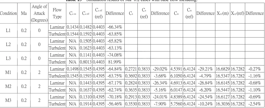
3.4.2.5 Location of Pressure Center

The location of pressure center determines the stability of the flying sounding rocket. We get it by taking the top of the nose of sounding rocket as the original point. In case of Ma=2.5, the location of pressure center is nearer the top of nose than other cases. The difference between the location of pressure center using turbulent flow model with the reference data is 5.48%. In cases of Ma=0.9, 1.1 and 1.5, the difference between the location of pressure center using turbulent flow model with the reference data are less than 4%. In the cases of supersonic and transonic using turbulent flow model, when the velocity becomes larger, the location of pressure center becomes smaller. It means that the rocket is more stable in transonic than in supersonic in the regime of Ma=0.9 to 2.5. In cases of subsonic, the difference between the location of pressure center using both flow model with the reference data are less than 5%. Because Xcp =Cm Cn, and the normal-force coefficients and the pitching-moment coefficients we discuss previously are not very close to the reference data, that the differences are less than 5% is not very reliable.

(35)

Chapter 4 Conclusions and Recommendation of Future

Work

4.1 Conclusion Remarks

The current study can summarize as follows:

1. We can accurately predict the physical properties in supersonic cases, and less accurate in transonic cases. In subsonic cases, because there are oscillation in the base flow, we still can not predict the physical properties accurately.

2. When Re<105_{, and Re>10}6_{, we can use laminar and turbulent flow model}

respectively. When 105_<Re<106_{, we can consider it as the transitional regime.}

4.2 Recommendation of Future Work

1. To simulate aerodynamics properties using different nose shape, such as 1/2 power series nose cone shape, and compare the results with the conical nose cone shape.

(36)

References

[1] Barth, T.J., “Recent Development in High Order K-Exact Reconstruction on Unstructured Meshes,” AIAA Paper 93-0668, 1993.

[2] Chen, Y.S., “An Unstructured Finite Volume Method for Viscous Flow Computations,” 7th International Conference on Finite Element Methods in Flow Problems, Feb. 3-7, 1989, University of Alabama in Huntsville, Huntsville, Alabama.

[3] Chen, Y.S., ”UNIC-UNS USER’S MANUAL”.

[4] Fumiya Togashi and et al., “CFD computations of NAL experimental airplane with rocket booster using overset unstructured grids,” International Journal for Numerical Methods in Fluids 2005; 48: 801-818.

[5] J. Reuther, “Aerodynamic Shape Optimization of Supersonic Aircraft Configurations via an Adjoint Formulation on Distributed Memory Parallel Computers,” Computer & Fluids 28 (1999) 675-700.

[6] Matthew Ross Smith, Personal communication.

[7] Paulo Moraes Jr., “Experimental Investigation of the Base Flow and Base Pressure of a Clustered Launch Vehicle.” Acta Astronautica Vol. 48, No. 5-12, pp. 485-489, 2001.

(37)

[8] Saad, Y. and Schultz, M.H., “GMRES: A Generalized Minimal Residual Algorithm for solving Nonsymmeric Linear Systems,” SIAM J. Sci. Stat. Comput., Vol. 7(3), pp. 856-869, 1986.

[9] Van Der Vorst, H.A., “Bi-CFSTAB: A Fast and Smoothly Converging Variant of Bi-CG for the solution of Nonsymmetric Linear Systems,” SIAM J. Sci. Stat. Comput., Vol. 13(2), pp. 631-644, 1992.

(38)

Tables

Table 1 Flow conditions of minimum grid size convergence test

Case Minimal Grid Size (mm) Ma A.o.A. (degrees) Altitude (m) Viscosity (N*s/m2 ) Pressure (atm) Density (kg/m3 ) Temperature (K) 1 2 2 1 3 0.4 4 0.1 2.5 0 10000 1.36E-05 0.2616 0.4135 223.27

Table 2 Simulation conditions of minimum grid size convergence test

Case Minimal Grid Size (mm) Number of Cells

Time Steps for Steady

(Time Step Size) CPUs Computation Time (hrs)

1 2 450,234 4,000 (2.6E-6) 8 3.99

2 1 467,118 8,000 (1.3E-6) 8 8.2

3 0.4 484,002 50,000 (5.2E-7) 16 35.73

4 0.1 517,770 60,000 (1.3E-7) 16 38.71

Table 3 The results of minimum grid size convergence test

Case Minimal Grid Size (mm) Axial Force (N) CA CA (reference) difference 1 2 702.300 0.343 12.22% 2 1 715.180 0.3493 10.61% 3 0.4 713.857 0.3487 10.78% 4 0.1 709.455 0.3465 0.3908 11.33%

(39)

Table 4 Flow conditions of comparison of laminar model and turbulent model

Case Condition Ma A.o.A. (Degrees) Altitude (m) Viscosity (N*s/m2 ) Pressure (atm) Density (kg/m3 ) Temperature (K) ReD 1 A 2.5 0 10000 1.359E-05 0.26160 0.41350 223.27 3.42E+06 2 C1 1.5 0 5000 1.536E-05 0.53356 0.73640 255.71 3.46E+06 3 C2 1.5 0 15000 1.322E-05 0.11955 0.19480 216.58 9.78E+05 4 E1 1.1 0 2000 1.637E-05 0.78480 1.00700 275.04 3.37E+06 5 E2 1.1 0 20000 1.322E-05 0.05458 0.08891 216.65 3.27E+05 6 G1 0.9 0 2000 1.637E-05 0.78480 1.00700 275.04 2.76E+06 7 G2 0.9 0 20000 1.322E-05 0.05458 0.08891 216.65 2.68E+05 8 I1 0.5 0 0 1.702E-05 1.00000 1.22500 288.09 1.84E+06 9 I2 0.5 0 15000 1.322E-05 0.11955 0.19480 216.58 3.26E+05 10 I3 0.5 0 24000 1.344E-05 0.02934 0.04694 220.58 7.80E+04 11 L1 0.2 0 0 1.702E-05 1.00000 1.22500 288.09 7.35E+05 12 L2 0.2 0 15000 1.322E-05 0.11955 0.19480 216.58 1.30E+05 13 L3 0.2 0 24000 1.344E-05 0.02934 0.04694 220.58 3.12E+04

Table 5 Simulation condition of comparison of laminar flow model and turbulent

flow model Case Number

of Cells

Number of

Time Step Time Step Size CPUs

Computation Time (hrs) 1 1.3E-06 2 2.0E-06 3 467,118 2.2E-06 9.5 4 2.7E-06 5 3.0E-06 6 3.3E-06 7 3.7E-06 8 5.8E-06 9 6.7E-06 10 6.7E-06 11 1.4E-05 12 1.6E-05 13 899,802 10,000 1.6E-05 8 22

(40)

Table 6 Flow conditions of simulation choose from 3DOF trajectory simulation results. Condition Ma A.o.A. (degrees) Altitude (m) Viscosity (N*s/m2 ) Pressure (atm) Density (kg/m3 ) Temperature (K) A 2.5 0 10000 1.359E-05 0.26160 0.41350 223.27 B 2.5 1 10000 1.359E-05 0.26160 0.41350 223.27 C1 1.5 0 5000 1.536E-05 0.53356 0.73640 255.71 C2 1.5 0 15000 1.322E-05 0.11955 0.19480 216.58 D1 1.5 1 5000 1.536E-05 0.53356 0.73640 255.71 D2 1.5 1 15000 1.322E-05 0.11955 0.19480 216.58 E1 1.1 0 2000 1.637E-05 0.78480 1.00700 275.04 E2 1.1 0 20000 1.322E-05 0.05458 0.08891 216.65 F1 1.1 2 2000 1.637E-05 0.78480 1.00700 275.04 F2 1.1 2 20000 1.322E-05 0.05458 0.08891 216.65 G1 0.9 0 2000 1.637E-05 0.78480 1.00700 275.04 G2 0.9 0 20000 1.322E-05 0.05458 0.08891 216.65 H1 0.9 2 2000 1.637E-05 0.78480 1.00700 275.04 H2 0.9 2 20000 1.322E-05 0.05458 0.08891 216.65 I1 0.5 0 0 1.702E-05 1.00000 1.22500 288.09 I2 0.5 0 15000 1.322E-05 0.11955 0.19480 216.58 I3 0.5 0 24000 1.344E-05 0.02934 0.04694 220.58 J1 0.5 2 0 1.702E-05 1.00000 1.22500 288.09 J2 0.5 2 15000 1.322E-05 0.11955 0.19480 216.58 J3 0.5 2 24000 1.344E-05 0.02934 0.04694 220.58 K1 0.5 4 0 1.702E-05 1.00000 1.22500 288.09 K2 0.5 4 15000 1.322E-05 0.11955 0.19480 216.58 K3 0.5 4 24000 1.344E-05 0.02934 0.04694 220.58 L1 0.2 0 0 1.702E-05 1.00000 1.22500 288.09 L2 0.2 0 15000 1.322E-05 0.11955 0.19480 216.58 L3 0.2 0 24000 1.344E-05 0.02934 0.04694 220.58 M1 0.2 2 0 1.702E-05 1.00000 1.22500 288.09 M2 0.2 2 15000 1.322E-05 0.11955 0.19480 216.58 M3 0.2 2 24000 1.344E-05 0.02934 0.04694 220.58

(41)

Table 7 Simulation conditions of different angle of attack. Condition Ma A.o.A. (degrees) Altitude (m) Number of Cells Number of Time Step Time Step Size CPUs Computation Time (hrs) A 2.5 0 10000 1.3E-06 B 2.5 1 10000 1.3E-06 C1 1.5 0 5000 2.0E-06 C2 1.5 0 15000 2.2E-06 D1 1.5 1 5000 2.0E+00 D2 1.5 1 15000 467,118 2.2E-06 9.5 E1 1.1 0 2000 2.7E-06 E2 1.1 0 20000 3.0E-06 F1 1.1 2 2000 2.7E-06 F2 1.1 2 20000 3.0E-06 G1 0.9 0 2000 3.3E-06 G2 0.9 0 20000 3.7E-06 H1 0.9 2 2000 3.3E-06 H2 0.9 2 20000 647,406 3.7E-06 20 I1 0.5 0 0 5.8E-06 I2 0.5 0 15000 6.7E-06 I3 0.5 0 24000 6.7E-06 J1 0.5 2 0 5.8E-06 J2 0.5 2 15000 6.7E-06 J3 0.5 2 24000 6.7E-06 K1 0.5 4 0 5.8E-06 K2 0.5 4 15000 6.7E-06 K3 0.5 4 24000 6.7E-06 L1 0.2 0 0 1.4E-05 L2 0.2 0 15000 1.6E-05 L3 0.2 0 24000 1.6E-05 M1 0.2 2 0 1.4E-05 M2 0.2 2 15000 1.6E-05 M3 0.2 2 24000 899,802 10000 1.6E-05 8 27

(42)

Table 8 Simulation results of supersonic cases without base flow. Condition Ma Angle of Attack (Degrees) Flow

Type Ca on Ca off Ca off (ref) Difference Cn Cn (ref) Difference Cm Cm (ref) Difference Xcp (m) Xcp (ref) Difference

Laminar 0.2300 0.2341 0.3908 -40.10% A 2.5 0 Turbulent 0.3851 0.3891 0.3908 -0.43% Laminar 0.2305 0.2346 0.3908 -39.99% 0.1457 0.1516 -3.93% 2.2934 2.2143 3.57% 15.7444 14.6046 7.80% B 2.5 1 Turbulent 0.3857 0.3898 0.3908 -0.28% 0.1528 0.1516 0.77% 2.3538 2.2143 6.30% 15.4052 14.6046 5.48% Laminar 0.3178 0.3241 0.5424 -40.26% C1 1.5 0 Turbulent 0.5152 0.5214 0.5424 -3.87% Laminar N/A 0.3404 0.5424 -37.25% C2 1.5 0 Turbulent N/A 0.5571 0.5424 2.70% Laminar 0.3180 0.3243 0.5422 -40.19% 0.1816 0.1880 -3.45% 3.2354 3.1577 2.46% 17.8208 16.7929 6.12% D1 1.5 1 Turbulent 0.5157 0.5219 0.5422 -3.73% 0.2105 0.1880 11.94% 3.6287 3.1577 14.92% 17.2402 16.7929 2.66% Laminar N/A 0.3418 0.5422 -36.96% 0.1850 0.1880 -1.63% 3.3043 3.1577 4.65% 17.8637 16.7929 6.38% D2 1.5 1 Turbulent N/A 0.5580 0.5422 2.92% 0.2113 0.1880 12.36% 3.6437 3.1577 15.39% 17.2459 16.7929 2.70%

(43)

Table 9 Simulation results of transonic cases without base flow. Condition Ma Angle of Attack (Degrees) Flow Type Ca on Ca off Ca off

(ref) Difference Cn Cn (ref) Difference Cm Cm (ref) Difference Xcp (m) Xcp (ref) Difference

Laminar 0.3748 0.3819 0.5499 -30.55% E1 1.1 0 Turbulent 0.5665 0.5735 0.5499 4.30% Laminar N/A 0.4175 0.5499 -24.08% E2 1.1 0 Turbulent N/A 0.6578 0.5499 19.63% Laminar 0.3744 0.3814 0.5491 -30.54% 0.4138 0.4243 -2.46% 7.6945 7.3924 4.09% 18.5928 17.4228 6.72% F1 1.1 2 Turbulent 0.5711 0.5782 0.5491 5.29% 0.4867 0.4243 14.70% 8.6190 7.3924 16.59% 17.7106 17.4228 1.65% Laminar N/A 0.4332 0.5491 -21.11% 0.4187 0.4243 -1.32% 7.7071 7.3924 4.26% 18.4069 17.4228 5.65% F2 1.1 2 Turbulent N/A 0.6647 0.5491 21.06% 0.4935 0.4243 16.32% 8.7615 7.3924 18.52% 17.7526 17.4228 1.89% Laminar 0.2112 0.2158 0.3901 -44.69% G1 0.9 0 Turbulent 0.4649 0.4695 0.3901 20.34% Laminar N/A 0.2569 0.3901 -34.14% G2 0.9 0 Turbulent N/A 0.5640 0.3901 44.57% Laminar 0.2120 0.2165 0.3894 -44.38% 0.3958 0.3892 1.69% 7.3376 6.8124 7.71% 18.5399 17.5032 5.92% H1 0.9 2 Turbulent 0.4690 0.4735 0.3894 21.62% 0.5058 0.3892 29.97% 9.1086 6.8124 33.71% 18.0067 17.5032 2.88% Laminar N/A 0.2734 0.3894 -29.78% 0.4122 0.3892 5.92% 7.6144 6.8124 11.77% 18.4710 17.5032 5.53% H2 0.9 2 Turbulent N/A 0.5705 0.3894 46.52% 0.5202 0.3892 33.65% 9.4100 6.8124 38.13% 18.0905 17.5032 3.36%

(44)

Table 10 Simulation results of Ma=0.5 cases without base flow. Condition Ma Angle of Attack (Degrees) Flow Type Ca on Ca off Ca off

(ref) Difference Cn Cn (ref) Difference Cm Cm (ref) Difference Xcp (m) Xcp (ref) Difference

Laminar 0.2233 0.2281 0.4106 -44.46% I1 0.5 0 Turbulent 0.4862 0.4910 0.4106 19.57% Laminar N/A 0.2692 0.4106 -34.43% I2 0.5 0 Turbulent N/A 0.5659 0.4106 37.83% Laminar N/A 0.3243 0.4106 -21.01% I3 0.5 0 Turbulent N/A 0.6931 0.4106 68.78% Laminar 0.2233 0.2280 0.4098 -44.36% 0.3921 0.3710 5.70% 7.3383 6.3749 15.11% 18.7147 17.1847 8.90% J1 0.5 2 Turbulent 0.4957 0.5005 0.4098 22.12% 0.3966 0.3710 6.90% 6.9023 6.3749 8.27% 17.4059 17.1847 1.29% Laminar N/A 0.2769 0.4098 -32.44% 0.3840 0.3710 3.53% 7.1032 6.3749 11.42% 18.4957 17.1847 7.63% J2 0.5 2 Turbulent N/A 0.5763 0.4098 40.62% 0.3698 0.3710 -0.33% 6.2545 6.3749 -1.89% 16.9155 17.1847 -1.57% Laminar N/A 0.3391 0.4098 -17.25% 0.3477 0.3710 -6.28% 6.1699 6.3749 -3.22% 17.7465 17.1847 3.27% J3 0.5 2 Turbulent N/A 0.7060 0.4098 72.27% 0.3054 0.3710 -17.68% 4.7304 6.3749 -25.80% 15.4911 17.1847 -9.86% Laminar 0.2197 0.2245 0.4087 -45.08% 0.8437 0.8072 4.53% 15.8573 14.0321 13.01% 18.7939 17.3842 8.11% K1 0.5 4 Turbulent 0.4995 0.5042 0.4087 23.37% 0.8894 0.8072 10.19% 15.6226 14.0321 11.33% 17.5649 17.3842 1.04% Laminar N/A 0.2916 0.4087 -28.66% 0.8402 0.8072 4.10% 15.5026 14.0321 10.48% 18.4504 17.3842 6.13% K2 0.5 4 Turbulent N/A 0.5824 0.4087 42.49% 0.8415 0.8072 4.25% 14.4741 14.0321 3.15% 17.2007 17.3842 -1.06% Laminar N/A 0.3792 0.4087 -7.21% 0.8129 0.8072 0.72% 14.4570 14.0321 3.03% 17.7834 17.3842 2.30% K3 0.5 4 Turbulent N/A 0.7171 0.4087 75.44% 0.7408 0.8072 -8.23% 12.0410 14.0321 -14.19% 16.2546 17.3842 -6.50%

(45)

Table 11 Simulation results of Ma=0.2 cases without base flow. Condition Ma Angle of Attack (Degrees) Flow Type Ca on Ca off Ca off (ref) Difference Cn Cn (ref) Difference Cm Cm

(ref) Difference Xcp (m) Xcp (ref) Difference

Laminar 0.1368 0.1710 0.4403 -61.16% L1 0.2 0 Turbulent 0.4270 0.4613 0.4403 4.76% Laminar N/A 0.2304 0.4403 -47.68% L2 0.2 0 Turbulent N/A 0.5783 0.4403 31.33% Laminar N/A 0.2960 0.4403 -32.77% L3 0.2 0 Turbulent N/A 0.8182 0.4403 85.82% Laminar 0.1443 0.1784 0.4395 -59.40% 0.4387 0.3833 14.45% 8.2854 6.4124 29.21% 18.8857 16.7282 12.90% M1 0.2 2 Turbulent Laminar N/A 0.2510 0.4395 -42.88% 0.4402 0.3833 14.85% 8.2491 6.4124 28.64% 18.7379 16.7282 12.01% M2 0.2 2 Turbulent Laminar N/A 0.3223 0.4395 -26.65% 0.4278 0.3833 11.59% 7.8115 6.4124 21.82% 18.2609 16.7282 9.16% M3 0.2 2 Turbulent

(46)

Table 12 Simulation results of Ma=0.5 cases with base flow including. Condition Ma Angle of Attack (Degrees) Flow Type Ca on Ca off Ca off (ref) Difference Cn Cn (ref) Difference Cm Cm

Laminar 0.1688 0.1736 0.4106 -57.73% I1 0.5 0 Turbulent 0.3959 0.4006 0.4106 -2.43% Laminar N/A 0.2011 0.4106 -51.02% I2 0.5 0 Turbulent N/A 0.4653 0.4106 13.31% Laminar N/A 0.2088 0.4106 -49.16% I3 0.5 0 Turbulent N/A 0.5937 0.4106 44.59% Laminar 0.1684 0.1731 0.4098 -57.76% 0.2823 0.3710 -23.90% 4.7664 6.3749 -25.23% 16.8832 17.1847 -1.75% J1 0.5 2 Turbulent 0.4043 0.4091 0.4098 -0.19% 0.3729 0.3710 0.52% 6.1473 6.3749 -3.57% 16.4862 17.1847 -4.06% Laminar N/A 0.2035 0.4098 -50.35% 0.2768 0.3710 -25.37% 4.5893 6.3749 -28.01% 16.5769 17.1847 -3.54% J2 0.5 2 Turbulent N/A 0.4749 0.4098 15.88% 0.3647 0.3710 -1.69% 5.9887 6.3749 -6.06% 16.4216 17.1847 -4.44% Laminar N/A 0.2497 0.4098 -39.07% 0.2830 0.3710 -23.71% 4.6389 6.3749 -27.23% 16.3919 17.1847 -4.61% J3 0.5 2 Turbulent N/A 0.6052 0.4098 47.67% 0.3655 0.3710 -1.47% 5.9611 6.3749 -6.49% 16.3085 17.1847 -5.10% Laminar 0.1715 0.1762 0.4087 -56.88% 0.6250 0.8072 -22.57% 10.8304 14.0321 -22.82% 17.3278 17.3842 -0.32% K1 0.5 4 Turbulent 0.4132 0.4179 0.4087 2.25% 0.7784 0.8072 -3.56% 12.9272 14.0321 -7.87% 16.6067 17.3842 -4.47% Laminar N/A 0.2326 0.4087 -43.09% 0.6630 0.8072 -17.86% 11.3926 14.0321 -18.81% 17.1839 17.3842 -1.15% K2 0.5 4 Turbulent N/A 0.4867 0.4087 19.09% 0.7630 0.8072 -5.47% 12.6116 14.0321 -10.12% 16.5288 17.3842 -4.92% Laminar N/A 0.3104 0.4087 -24.05% 0.6696 0.8072 -17.04% 11.1101 14.0321 -20.82% 16.5911 17.3842 -4.56% K3 0.5 4 Turbulent N/A 0.1786 0.4087 -56.31% 0.7548 0.8072 -6.49% 12.5281 14.0321 -10.72% 16.5980 17.3842 -4.52%

(47)

Table 13 Simulation results of Ma=0.2 cases with base flow including. Condition Ma Angle of Attack (Degrees) Flow Type Ca on Ca off Ca off (ref) Difference Cn Cn (ref) Difference Cm Cm

Laminar 0.1434 0.1482 0.4403 -66.34% L1 0.2 0 Turbulent 0.1544 0.1592 0.4403 -63.85% Laminar N/A 0.1505 0.4403 -65.82% L2 0.2 0 Turbulent N/A 0.1623 0.4403 -63.13% Laminar N/A 0.1141 0.4403 -74.08% L3 0.2 0 Turbulent N/A 0.8013 0.4403 81.99% Laminar 0.1498 0.1545 0.4395 -64.84% 0.2721 0.3833 -29.02% 4.5391 6.4124 -29.21% 16.6829 16.7282 -0.27% M1 0.2 2 Turbulent 0.1545 0.1593 0.4395 -63.75% 0.3692 0.3833 -3.68% 6.1050 6.4124 -4.79% 16.5347 16.7282 -1.16% Laminar N/A 0.1443 0.4395 -67.17% 0.2824 0.3833 -26.34% 4.6913 6.4124 -26.84% 16.6145 16.7282 -0.68% M2 0.2 2 Turbulent N/A 0.1637 0.4395 -62.74% 0.3635 0.3833 -5.16% 6.0147 6.4124 -6.20% 16.5447 16.7282 -1.10% Laminar N/A 0.1310 0.4395 -70.18% 0.2913 0.3833 -24.01% 4.8389 6.4124 -24.54% 16.6127 16.7282 -0.69% M3 0.2 2 Turbulent N/A 0.1914 0.4395 -56.46% 0.3530 0.3833 -7.90% 5.7560 6.4124 -10.24% 16.3036 16.7282 -2.54%

(48)

Figures

(49)

Figure 1.2 Generic supersonic transport configuration SYN87-MB Grid Structure:

180 Blocks

Figure 1.3 Generic supersonic transport configuration SYN87-MB solution

pressure coefficient (Mach=2.2 _α ₌₃_.₁₅0 ₌₀_.₁₀₅

L

(50)

(51)

Figure 1.5 Transonic flow over the satellite launch vehicle.

Figure 1.6 NAL jet-powered experimental airplane with a small rocket booster.

(52)

Figure 1.8 Computed pressure contours of the airplane and booster and enlarged

views around the intake with and without a small booster: (A) and (C)M_∞ =1.4, 0

. 5 =

(53)

Figure 2.1 Unstructured control volume.

Figure 3.1 The Results of 3DOF trajectory simulation.

(54)

(A)

(55)

(C)

(D)

Figure 3.3 Typical grid distribution of aerodynamics simulation of sounding rocket.

(A) grid distribution of symmetric plane, (B) grid distribution of external flow field, (C) grid distribution of body surface, (D) grid distribution of fin surface.

(56)

(A)

(B)

(57)

(D)

Figure 3.4 The comparison of minimum grid size: (A)Δx_min =2mm,

(B)Δx_min =1mm, (C)Δx_min =0.4mm, (D)Δx_min =0.1mm.

(A)

(58)

(D) (E)

(F) (G)

(59)

(J) (K)

(L) (M)

Figure 3.5 Aerodynamics simulation results of laminar flow model and turbulent

model, (A) case 1, (B) case 2, (C) case 3, (D) case 4, (E) case 5, (F) case 6, (G) case 7, (H) case 8, (I) case 9, (J) case 10, (K) case 11, (L) case 12, (M) case 13.

(60)

(A)

(61)

(C)

Figure 3.6 Difference of axial-force coefficients between numerical results and

reference data, (A) supersonic cases, case 1~3, (B) transonic cases, case 4~7, (C) subsonic cases, case 8~13.

(62)

Figure 3.7 Difference of axial-force coefficient between numerical results and

(63)

Figure 3.8 The density, pressure and Mach number distributions at Ma=2.5,

A.o.A.=0 degree, H=10000 m

(64)

(65)

(66)

(67)

(68)

(69)

(70)

(71)

低空探空火箭的氣動力性質模擬

國 立 交 通 大 學

機 械 工 程 學 系

碩 士 論 文

Simulation of Aerodynamics Properties of

a Low-Altitude Sounding Rocket

低空探空火箭的氣動力性質模擬

研究生：古必任

指導教授：吳宗信 博士

低空探空火箭的氣動力性質模擬

Simulation of Aerodynamics Properties of

a Low-Altitude Sounding Rocket

研 究 生：古必任

Student：Bi-Ren Gu

指導教授：吳宗信 博士

Advisor：Dr. Jong-Shinn Wu

國立交通大學

機械工程學系

碩 士 論 文

A Thesis

Submitted to Department of Mechanical Engineering

College of Engineering

National Chiao Tung University

in Partial Fulfillment of the Requirements

for the Degree of

Master of Science

In

Mechanical Engineering

July 2009

Hisnchu, Taiwan

西元 2009 年 7 月

低空探空火箭的氣動力參數模擬

學生：古必任

指導教授：吳宗信博士

國立交通大學機械工程學系

摘要

探空火箭(sounding rocket)是太空運載工具的一種，採取省去

導引及控制系統來降低成本，利用機翼或裙狀外型來進行氣動力控

制，保持火箭穩定飛行。探空火箭主要功能為運送精密探測儀器進入

地球軌道進行自然現象的探測行為。探空火箭飛行在不同的階段：在

不同速度情況下有次音速、穿音速、超音速到極超音速等階段；大氣

密度也隨著不斷攀升的高度而變動，此時火箭會經歷連續流場、過度

流場以及稀薄氣體流場。在探空火箭的氣動以及熱傳系統設計領域

中，各具特色的飛行環境的所造成不同的氣動及熱傳模擬方法的建構

是非常重要的。UNIC-UNS 是一套求解 Navier-Stokes 方程式的程式，

在這份研究當中，我們利用這個程式來模擬探空火箭在不同飛行階段

與各具特色的大氣環境中，氣動及熱傳情況。我們首先必須做網格測

試來選擇最有效率的網格數量，再利用此網格來進行不同飛行階段：

不同的馬赫數、大氣密度以及飛行攻角的氣動力性質模擬。最後再比

較層流模組跟紊流模組模擬出來的結果。由結果可以看出，當雷諾數

小於 10

時，使用層流模組模擬出來的結果較準，當雷諾數大於 10

時，使用紊流模組模擬出來的結果較準，而雷諾數介於這兩者中間的

流場條件，則視為過度區，用此兩種流場型態去模擬都不能夠得到非

常準確的結果。

Simulation of Aerodynamics Properties of

a Low-Altitude Sounding Rocket

Student: Bi-Ren Gu

Advisor: Dr. Jong-Shinn Wu

Department of Mechanical Engineering

National Chiao-Tung University

Abstract

誌謝

本篇論文能夠完成，首先要感謝指導老師吳宗信教授的指導，在研究

上，幫我指引出研究的方向，使我有目標可以追求，並且教導我做人

做事該有的方法及態度。另外要感謝黃俊誠老師以及陳彥升博士，感

謝他們在忙碌之餘仍抽空幫我解決研究上的疑難雜症。感謝洪捷粲、

邱沅明、柳志良、蘇正勤、鄭凱文、林昆模、李允民、吳玟琪、胡孟

樺、林雅茹、林宗漢、江明鴻、劉育宗、鄭承志、曾坤璋、連又永等

諸位學長姐，感謝他們在研究及生活上的關心及照顧。感謝穎志、逸

民、俊傑、振庭等同學兩年來學業及生活上的相互扶持。感謝子豪、

皓遠、其璋、瑞祥、柏村、冠融等學弟的幫忙及協助。最後要感謝在

我所有的家人們以及佳芳在我求學階段中給予我的支持，讓我在學業

上無後顧之憂，專心於研究。

必任 謹致

于新竹交大

2009 年 8 月

Table of Contents

List of Tables

List of Figures

國立交通大學

機械工程學系

碩士論文

指導教授：吳宗信博士

研究生：古必任

指導教授：吳宗信博士

碩士論文

必任謹致

₍

₎