Parallel Computing 16 (1990) 41-57
North-Holland 41
Structured partitioning of concurrent
programs for execution
on multiprocessors *
Chien-Min WANG and Sheng-De W A N GDepartment of Electrical Engineerin~ National Taiwan University, Taipei 10764, Taiwan Received 8 June 1989
Revised 22 January 1990
Abstract. In this paper, the problem of partitioning of parallel programs for execution on multiprocessors is investigated. By assuming run-time scheduling approaches, the static partitioning problems are formulated and solved in the context of a structured program representation model, in which a program is assumed to be composed of paratlel loops. The structured partitioning problem is then defined as the problem of partitioning each parallel loop into appropriate number of tasks such that the program execution time is minimized in some sense. The worst case of the program execution cost is adopted as the minimization criterion, so the results obtained in this paper are guaranteed to be within some performance bound. Two algorithms are developed to solve this problem. The first algorithm using a prune-and-search technique can fmd the optimal partition, while the second algorithm can ~btain a near optimal partition for the simplified partition problem in linear time. It is proved that the cost of the partition generated by the linear time algorithm is at most twice the cost of the optimal partition.
Keywords. Program partitioning, Shared memory multiprocessor, Scheduling mechanism, Structured partition problem, Simplified structured partition problem, Cost analysis.
1. Introduction
One of the trends in developing future general-purpose supercomputers is toward the shared memory multiprocessors. However, a serious problem arises when we attempt to execute parallel programs on these multiprocessors. The overheads of communication, synchronization, and scheduling become a bottleneck to parallel processing [9,10]. Let the granularity of a parallel program be defined as the average execution time of a sequential unit of computation in the program without inter-processor synchronization or communication. For a multi- processor system, there exists a minimum program granularity below which the performance degrades significantly due to frequent synchronizations and communications. On the other hand, the coarser granularity means the more parallelism lost and the attempt to minimize such overheads usually results in reducing the degree of program parallelism.
In order to obtain an appropriate granularity, the technique of program partitioning was proposed [2,13,18]. Program partitioning is the process of partitioning a parallel program into tasks in such a way that the inter-task communication and synchronization overheads are minimized and the resulting tasks can be scheduled onto the available processors without excessive scheduling overheads. However, finding the optimal partition is a nontrivial optimiza-
42 C.-M. Wan& $.-D. Wang / Structured partitioning of concurrent programs
tion problem. Most instances of this optimization problem have been proved to be NP-com- plete [18,19].
One solution to this problem is the explicit partitioning approach which is done by the programmers, but there are several drawbacks about this approach. First, this approach places a tremendous burden on programmers - both for correctness and performance. Second, the partition defined by the programmers is unlikely to be near the optimal partition. Third, the program written with an explicit partition may not be portable in performance to difference multiprocessors. Finally, the way to express the partitioning of a parallel program is dependent on the programming language used.
In order to free programmers from the above inconveniences, the development of a software program that can automatically partition parallel programs into tasks for the target multi- processor is desired. However, the complexity of this problem has led the computing commun- ity to adopt heuristic approaches. A major disadvantage of heuristic approaches is that they are based on some conjectures or experiences, so there is no gnarantee about the worst-case performance of these algorithms. I n this paper, we propose an alternative approach. Since it is difficult or impossible to find a universal solution for the general partition problem, we concentrate our attentions on two problems called the Structured Partition Problem and the Simplified Structured Partition Problem. Then two algorithms will be presented. The first algorithm uses a prune-and-search technique to reduce the time in searching the optimal partition for the Structured Partition Problem. The second algorithm will generate a near optimal partition for the Simplified Structured Partition Problem in linear time. The cost of the partition generated by the linear time algorithm is proved to be at most twice the cost of the optimal partition.
The rest of this paper is organized as follows. Section 2 gives some background information and the necessary definitions. Section 3 defines the Structures Partition Problem and the Simplified Structured Partition Problem. The two algorithms will be presented in Sections 4 and 5, respectively. Finally, conclusions are given in Section 6.
2. ~ a ~ u n d
There are three possibilities for automatic partitioning and scheduling [18]. They are the run-time partitioning and run-time scheduling approach, the compile-time partitioning and run-time scheduling approach, and the compile-time partitioning and compile-time scheduling approach. In this paper, we adopt the second approach. This approach is very attractive because it provides a good trade-off between the inaccurate estimate of the compile-time analysis and the extra overhead of the run-time analysis. In addition, we shall study the partition problem only.
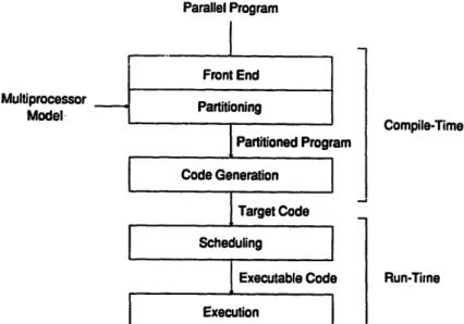
As shown in Fig. 1, an automatic partitioner takes a given parallel program and a target multiprocessor model as inputs and produces a partitioned program as output. Before partition- ing the parallel program, a front end will transform the parallel program into an program representation suitable for the process of partitioning. After the partitioned program is produced, a code generator is used to generate the target code. At run time, the scheduler picks ready tasks and assigns them to available processors for execution.
2.1 The multiprocessor model
The target multiprocessor is a tightly coupled multiprocessor. It is assumed that each processor has its own local memory and processors communicate through shared memory
C.-M. Wang, $.-D. Wang / Structured partitioning of concurrent programs
43
! Multiprocessor[
Model- ] Parallel ProgramI
Front End Partitioning I Partitioned Program Code Generation[
Target Code Scheduling I Executable Code Execution Compile-Time Run-TimeFig. 1. The compile-time partitioning and run-time scheduling approach.
modules. Neither processors nor shared memory modules are distinguishable from their neighbors. Each shared memory module is capable of being accessed by any processor through the interconnection network. Systems in this class include the Alliant FX series, the Denelcor HEP, the University of Illinois Cedar system, the New York University Ultracomputer, and the IBM RP3 multiprocessor.
The oniy inter-processor interactions considered are the task scheduling and the data communication (synchronization is treated as a special case of communication). All other inter-processor interactions which may arise in the real multiprocessor systems, such as I / O contention for system resources and distribution of program code are ignored. Access to the shared memory modules is assumed to be deterministic in that either fetches or stores from a single processor are processed in the order they are issued. This means that either fetches or stores within a processor are done serially, or that an equivalent ordering is imposed on data accesses.
The performance of the target multiprocessor can be characterized by a 5-tuple M = (P, R, W, S, E). Among these, P is the number of processors in the target multiprocessor. The function R is the communication overhead function for reading data. It estimates the time required to fetch data from a shared memory module to a local memory through the interconnection network. The function W is the communication overhead function for writing data. It estimates the time required to store data from a local memory to a shared memory module through the interconnection network. The function S is the scheduling overhead function. It estimates the scheduling overhead incurred by a processor when it begins execution of a new task. The function E estimates the time reqmred to complete the computation of a program segment.
2.2 The program representation
The parallel program is represented as a program graph based on the Graphical Representa- tion (GR) [18]. In the program graph, parallelism is explicitly specified. As discussed in the above, a front end transforms parallel programs into program graphs and computes those attributes needed for partitioning. For each transformed program, it is assumed that each branch of an IF or GOTO statement is assigned a branching probability by the user, or
44 C.-M. Wang, $.-D. Wang / Structured partitioning of concurrent programs
automatically determined by the front end. Each loop is automatically normalized. Like the branching probabilities, unknown loop upper bounds are either defined by the user, or automatically determined by the front end.
In the program graph, a program is composed of a set of function definitions. Each function definition consists of a directed graph representing its computations. A directed graph is a 2-tuple
G-(V,
A) where V is a set of nodes and A is a set of arcs. The nodes in V represent the computations of that function and the arcs in A represent communications and synchroni- zations between nodes, which enforce the precedence constraints.There are four kinds of nodes. A simple node represents an indivisible sequential computa- tion like a simple statement. A parallel node represents the parallel iterative construct like DOALL statements. A function node represents a function call to a function. A compound node contains a set of graph-frequency pairs and is used to denote any complex program structures. Each execution of a compound node is an arbitrary sequential execution of its subgraphs, so that subgraphs may be executed any number of time in any order. If we consider subgraphs to be like basic blocks, this general definition corresponds to a sequential flow graph which is complete and thus includes all other flow graphs (e.g. IF, WHILE). In general a program graph may contain nested DOALL loops. A program graph is a simple program graph if it does not contain nested DOALL loops.
Arcs represent the precedence constraints between nodes. In modeling precedence graphs, two language constructs are often used in parallel languages. One is the concurrent construct of the block-structured language originally proposed by Dijkstra and the other is the F O R K / J O I N construct. The latter construct has the drawback that, like the GOTO statements in the sequential programs, the F O R K / J O I N statements make the parallel programs hard to read and understand. Therefore, in this paper we consider the concurrent construct only. In this case, the set of n statements S 1, $2,.--, S,, that can be executed concurrently can be expressed as the statement PAR.BEGIN $1; $2; ... ; Sn PAP, END. Although the concurrent construct alone is not powerful enough to model all possible precedence graphs, it is well suited to structured programming.
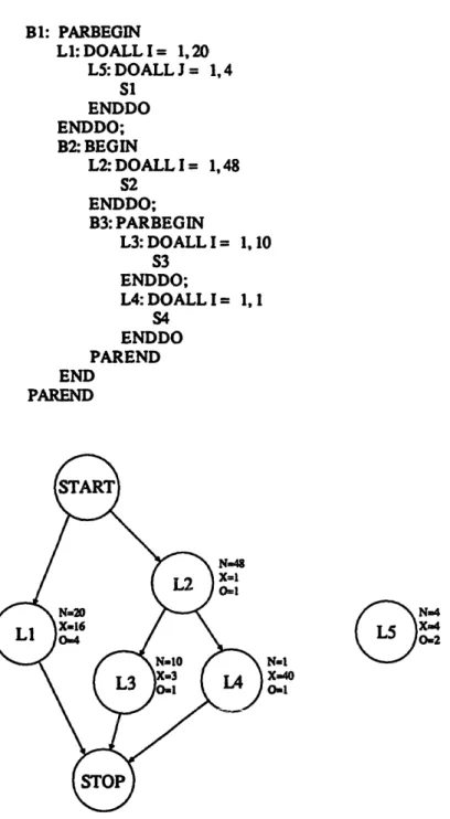
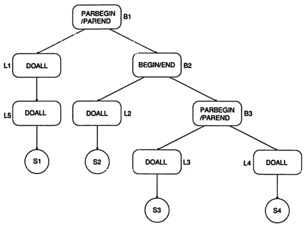
Fig. 2 shows the example program used throughout this paper and its program graph. Although the program graph representation is useful for representing programs written in different languages, it is inconvenient in illustrating our partitioning algorithms. We shall use the parse tree representation instead. In a parse tree, leave nodes represent simple nodes, while internal nodes represent constructs like DOALL constructs, B E G I N / E N D constructs, and PARBEGIN/PAREND constructs. For a structured program graph that can be modeled by the PARBEGIN/PAREND construct and the B E G I N / E N D construct, it is easy to generate the parse tree of a program from its program graph [13]. The parse tree of the example program is shown in Fig. 3.
2.3 The partitioned program
The context switching, necessary for synchronization, and the task migration, necessary for load-balancing are two major sources of scheduling overhead. If they occur frequently, the scheduling overhead incurred may well undo the potential speedup obtained by parallel processing. This problem will be greatly simplified if tasks are functional in nature. A functional task can only be scheduled when all its inputs are available. Once scheduled it can run to completion without interacting with other tasks. The context switching for synchroniza- tion and the task migration for load balancing are no longer necessary during the execution period of a functional task. Scheduling overhead is only incurred when a task starts execution and can be easily predicted at compile time. Note that, for a functional task, there is only one
C.-M. WanK $.-D. Wang / Structured partitioning of concurrent programs 45 B 1: PARBEGIN L h DOALL I - 1, 20 LS: DOALL J - 1, 4 SI ENDDO ENDDO; B2: BEGIN L2: DOALL I -- 1, 48 $2 ENDDO; B3: PARBEGIN L3: DOALL I -- 1, 10 $3 ENDDO; L4: DOALL I --- 1, 1 $4 ENDDO PAREND END PAREND N=20 X=16 O ~ N=48 X=I 0=I lq=! X=40 0~1
Fig. 2. An example program and its program graph.
entry point and one exit point. We shall use T A S K B E G I N and T A S K E N D to denote the entry point and the exit point of a task.
Focusing on the partitioning of parallel loops, we may observe two types of parallelism: horizontal and vertical [16]. Horizontal parallelism results by simultaneously executing different iterations of the same parallel loop on different processors. Vertical parallelism, in turn, is the result of the simultaneous execution of two or more different loops. Now consider the following parallel loop:
L: DOALL I - 1, N
B
46 C-M. Wang, $.-D. Wang / Structured partitioning of concurrent programs
J /
DOALL 1
°°,.. )
PARBEGIN
IPAREND
]B1BEGIN/END I B2
O0,LL
I
I ==
L
=L
Fig. 3. The parse tree of the example program.
If this loop is partitioned into K tasks, the partitioned loop can be expressed as follows: L: DOALL T - 1, K TASKBEGIN DOSER I - 1, N , K B ENDDO TASKEND ENDDO
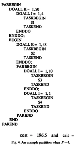
If a parallel loop L is partitioned as the above example, the partition of the loop L, denoted by HL, can be expressed as H L - {(L, K)}. A partition is structured if every task in this partition is obtained by partitioning some parallel node as the above example. Those parallel nodes partitioned are called primitive nodes. A structured partition of a parallel program can be defined as the union of partitions of primitive loops. Due to the restriction of functional tasks, parallelism between primitive nodes will be fully exploited while parallelism within a task will not be exploited. Therefore, in a structured partition, the precedence between tasks are the same as the precedence relations between primitive nodes. As an illustration, Fig. 4 and Fig. 5 give two structured partitions. Fig. 4 is an example partition that exploits all parallelism. Fig. 5 is the optimal partition generated by the algorithm proposed in Section 4.
2.4 The scheduling mechanism
The scheduling mechanism can have severe impacts on the performance of the multi- processor systems. The general scheduling problem has been proved to be NP-complete in the strong sense [8]. It has been shown that, in certain case of random task graphs, optimal schedules can be achieved by deliberately keeping one or more processors idle in order to better
C.-M. Wan~ S.-D. Wang / Structured partitioning of concurrent programs 47 PARBEGIN DOALL K-- 1, 20 DOALL J -- I, 4 TASKBEGIN Sl TASKEND ENDDO ENDDO; BEGIN DOALL K - 1, 48 TASKBEGIN $2 TASKEND ENDDO; PARBEGIN DOALL I - l, l0 TASKBEGIN S3 TASKEND ENDDO; DOALL I = l, 1 TASKBEGIN $4 TASKEND ENDDO PAREND END PAREND
cost - 196.5 and crit = 43
Fig. 4. An example partition when P -- 4.
utilize them in a later point. Detecting such anomalies, however, requires processing of the entire task graph in advance. Since this is not possible at run time, the luxury of deliberately keeping processors idle should not be permitted.
Therefore, we assume the following fist scheduling algorithm is used. For convenience, we define a macro-actor to be a dynamic invocation of a static task. The distinction between a macro-actor and a task is akin to the distinction between a process and a program. In the run-time scheduling model, each processor repeats the following steps serially and there is no opportunity for overlapping communication with computation:
1. pick a ready macro-actor 2. fetch the macro-actor's inputs 3. execute the macro-actor
4. store the macro-actor's outputs.
An important property of this scheduling model and other list scheduling algorithms is that there is no intentionally introduced idleness. This means that a processor never stay idle if there is a macro-actor ready for execution. Despite of this limitation, this scheduling model is not an obstacle to achieve linear speedup because it was proved [7] that th~ schedule generated by a list scheduling algorithm have a parallel execution time at most twice the optimal parallel execution time.
48 C.-M. Wangp S.-D. Wang / Structured partitioning of concurrent programs PARBEGIN D O A L L K - 1, 7 TASKBEGIN DOSEP I = K, 20, 7 DOSER J -- 1, 4 Sl ENDDO ENDDO TASKEND ENDDO; BEGIN D O A L L K = 1, 5 TASK.BEGIN DOSER I = K. 48, 5 $2 ENDDO TASKEND ENDDO; PARBEGIN TASKBEGIN DOSER I = 1, 10 $3 ENDDO; TASKEND TASIG3EGIN DOALL I = 1, 1 $4 ENDDO TASKEND PAREND END PAREND c o s t - - 157.25 and c r i t - 52
Fig. 5. The optimal partition when P -- 4.
3. Problem
For convenience, we define some notations to be used. Consider the execution of a program graph G under the partition H for a single set of inputs. TOTAL(G,/'/) is defined to be the total execution time of all macro-actors. CRIT(G, H) is defined as the critical path execution time of the run-time precedence graph, i.e. the total execution time of those macro-actors that lie on the critical path of the run-time precedence graph. Therefore, C R I T ( G , / / ) is the parallel execution time of the program on infinite number of processors. Let Tpar(P) denote the parallel execution time of the program on P processors under the run-time scheduling model described in the previous section. Then,
Tp~r(P)
approaches CRIT(G~ H) as the number of processors approaches infinity.The goal of program partitioning is to find the optimal partition which minimizes parallel execution time with limited number of processors in the presence of overhead. Since the scheduling of tasks is performed at run time, there is no way to know the parallel execution time of a partitioned program at compile time. Fortunately, based on the scheduling model defined in the previous section, a theorem presented by Sarkar [18] provides us a reasonable
C-M. Wang, $.-D. Wang / Structured partitioning of concurrent programs 49
cost function to evaluate the performance of a partitioned program. This theorem is stated below without proof.
Theorem 3.1.
P -
1CRIT(G,/'/) + ~ p TOTAL(G, H) ~< rpar(P ) ~ f f - ~ C R I T ( G , / / ) 2P
+ 1 T O T A L ( G , H).
Although different scheduling algorithms may generate different values of Tp~,(P), Theorem 3.1 provides bounds on Tpar(P ). Since the problem of finding a schedule with the smallest
Tpar(P) is
NP-complete [8], it is reasonable to use the worst-case performance instead of Tpar(P) as the cost function. Therefore we define the Structured Partition Problem and the Simplified Structured Partition Problem as follows.Definition. Let f ( H ) = ~ CRIT(G, H) + 1 TOTAL(G, H) be the cost of partition H.
Definition. The Structured Partition Problem is defined as follows. Given a program graph G--(V, A) and a multiprocessor model M ffi (P, R, W, S, E) as defined in the previous section, find a structured partition H of the program graph G such that f ( H ) is minimized.
Definition. The Simplified Structured Partitioned Problem is defined as follows. Given an simple program graph G = (IF, A) and a multiprocessor model M ffi (P, R , W, S, E), find a structured partition/I of the program graph G such that f(/'/) is minimized.
Note that, for a simple program graph, there are only two types of nodes: simple nodes and parallel nodes. Since a simple node can be treated as a parallel node with only one iteration, the processing of a simple node is the same as that of a parallel node. Therefore, there are only three types of internal nodes in the parse tree of a simple program graph. They are the PARBEGIN/PAREND nodes, the BEGIN/END nodes, and the DOALL nodes. Further- more, every DOALL node is a primitive node for a simple program graph since there is no nested loops.
4. The prune-and-search algorithm
In this section, we consider the Simplified Structured Partition Problem first and propose an algorithm to solve this problem. The algorithm is then extended to solve the Structured Partition Problem. Like the definitions of the total execution time and the critical path execution time of a program in the previous section, we can define the total execution time and the critical path execution time of a node in the parse tree in a similar manner. In the following we shall discuss the computation of the total execution time and the critical path execution time of an internal node in an bottom-up manner. First, consider parallel node V~ partitioned into K~ tasks. For a parallel node V~, we use the following notations: The partition of this parallel node is expressed as Hvi = {(V~, K~)}. N~ denotes the number of iterations of V~. R~ denotes the time to read input data of an iteration of V~ from the shared memory modules and W~ denotes the time to write the output data of an iteration of V~ to the shared memory modules. CR~ denotes the time to read the input data that are common for all iterations of V~ (e.g. scalar variables). E i denotes the time to perform the computation of an iteration of V~. The
50 C.-M. Wan& S.-D. Wang / Structured partitioning of concurrent programs
scheduling overhead incurred by scheduling a task of ~ is denoted by $~. Note that some tasks of V~ will contain [~/K~] iterations while others contain |NJK~] - 1 iterations. Since the input
data common for all iterations of V~ can be read only once for each task, the total execution time and the critical path execution time of this parallel node can be expressed as the following equations:
TOTAL(V~,//vi) = N~ *(E, + R , - C ~ + Wt) + K~ * ( S i + CRi)
=/v,. x, + K,.O,
O)
CRIT(E,//vt)f[~/K,|*(E,
+R , - CR, + ~ ) +
(S,+CR,)
= [ ~ / K , 1 , x~ + o,
(2)
where Xi - (E~ + Ri - CR~ + 14~) and O~ = Si + CRy.
Then consider a concurrent block of statements in the form of CB: PARBEGIN BI; B2; . . . ;
B n PAREND. By definition, the total execution time and the critical path execution time of this
concurrent block can be computed as follows. n
TOTAL(CB,/I,b) = E TOTAL(B~,//ei)
i=1
CRIT(CB,//,b) = m~CRIT(B,, ]'~Bi)
i=1 /I
where//cb-~ U //Bi" i = l
Finally consider a sequential block of statements in the form of SB: BEGIN B~; B2; ...; B,, END. By definition, the total execution time and the critical path execution time of this sequential block can be computed as follows:
n
TOTAL(SB, /'/,b)= ~ T O T A L ( B , , / / m ) i'-1
n
CRIT(SB,//sb) -- E CRIT(B,, ~r/Bi ) i - I
n where Heb = ~ / / B i "
i - I
Since there are only these three types of internal nodes in the parse tree of a simple program graph, we can compute the total execution time and the critical path execution time of a simple program graph by applying the above equations in an bottom-up manner when the partition is given. However, there are so many possible partitions such that an exhaustive search of all possible partitions is impossible. In the following we try to find some ways to prune those partitions that, no matter how many processors are available, they are not capable of being the optimal partition. For example, l e t / / t a n d / / 2 be two possible partitions of the program graph G. If TOTAL(G, Ht) < TOTAL(G,//2) and CRIT(G,//1) ~< CRIT( G, //2 ), we can conclude that, no matter how many processors are available, the partition
//2
will not be the optimal partition of the program graph G because f ( / / l ) < f ( / / 2 ) . The following theorem is ageneralization of this example.
Theorem 4.1. Let/'/opt denote the optimal partition of the program graph G. I f / / I and 1-12 are two possible partitions of some program segment B in the program graph G and TOTAL(B,//1)
C-M. Wang S.-D. Wang / Structured partitioning of concurrent programs 51
Proof. Suppose /'/2 C //opt. Since TOTAL(B, H1)<TOTAL(B,/-/2) and CRIT(B, Hi)~< CRIT(B,
11~), f(G,//o~-1112 + 1111)<f(G, Hopt). However, this contradicts the original
assumption. Therefore//2 4Z/'/opt. This completes the proof of Theorem 4.1. []Those partitions that can not be pruned by Theorem 4.1 are called candidate partitions. The optimal partition must be one of the candidate partitions. Given the number of processors available, we can find the optimal partition by searching all candidate partitions of the parallel program. Since the number of candidate partitions is far less than the number of possible partitions, the search of the optimal partition will become much faster. In the following discussion we shall assume the set of candidate partitions and their total execution times are stored in two arrays, called the candidate partition array and the candidate total-execution-time array, indexed by their critical path execution times. Let q'B, CPB and CTB denote the set of candidate partitions, the candidate partition array and the candidate total-execution-time array of an internal node B, respectively. CPB and CT B are defined as follows:
for an 17 e CI',[C T(B, 1I)] - 17.
for an 17 ¢ cr [C T(n, - T O T A L ( n ,
As an illustration, consider the parallel loop L3 in the example program. All possible partitions of L3 is shown in Fig. 6(a). After applying Theorem 4.1 to this example, its candidate partition array and candidate total-execution-time array can be computed and are shown in Fig. 6(b). Note that CPn[C] and CTB[C] are undefined for some value C. In order to make the seareh of the optimal partition more easily, we shall use the extended candidate partition array ECP and the extended candidate total-execution-time array ECT in our algorithm. Fig. 6(c) shows the extended candidate partition array and the extended candidate total-execution-time array ot L3. Formally, ECTB is defined as follows:
for all C: ECTB[C ] - min T O T A L ( B , / / ) . H
CRIT( B, /'/) ~ C
For all C, ECPn[C] ffi H where H is the partition whose total execution time is minimum among all partitions that satisfy CRIT( B, /'/) ~ C. In other words, ECPB[C] = H if and only if ECTB[C ] -- TOTAL(B, H). Note that the above definitions of ECP and ECT confirm with the definitions of CP and CT, i,e. for all / / ) ¢ q'e, ECPe[CRIT(B, / ' / ) ] - H and ECTB[CRIT (B, H ) ] - TOTAL(B, H). An important property of ECT is that it is nonincreas- ing, i.e. ECT[CI] >I ECT[Ca] if Ci < C2. In the following, we shall utilize this property to prune those partitions that are incapable of being the optimal partition and obtain the set of candidate partitions.
Now the problem is shifted to the computation of the extended candidate partition array and the extended candidate total-execution-time array of a parallel program. We shall compute these two array in an bottom-up manner. First consider a parallel node V~. By definition, for all
C>~+O,:
ECTvi [ C ] --- rain TOTAL( V~, Hv~ ) l'/vi CRIT0,'i, Hvi) ~ C - rain + K , , O , ) l~IKd* Xj+ 0 ~ C = . x, + [ o,)/x ll . o,
(3)
ECPvi[C] _{(~,
[lV]/[(C_Oi)/Xi]])}"
(4)52 C-M. Wang, $.-D. Wang / Structured partitioning of concurrent programs
The consider a concurrent block of statements. Utilizing the nonincreasing property of the the extended candidate total-execution-time array, we can compute the extended candidate partition array and the extended total-execution-time array of a concurrent block based on the following two theorems.
Theorem 4.2. For a concurrent block of statements in the form of CB: PARBEGIN
St; $2
PAREND, the following equations hold:
for all C:
ECTcb[C ] = ECTs,[C ] + ECTs2[C].
(5)
for all C: ECPcb [ C ] = ECPs, [ C ] U ECTs2 [ C 1. (6)
N= 10, X=3, O=1 K 1 2 3 4 5 6 7 8 9 10 TOTAL 31 32 33 34 35 36 37 38 39 40 CRIT 31 16 13 10 7 7 7 7 7 4 TOTAL (a) 4O 39 38 37 36 35 34 33 32 K=10 x K=9 x K=8 x K : 7 x K : 6 x K=5 x K=4 l( K=3 x 4 7 10 13 K=2 x 16 K=I x 31 CRIT TOTAL (b) 40 39 38 37 ;.~6 35 34 33 32 31 K = I 0 o K=5 o K=4 o K.--3 o K--.2 o K=I o 4 7 10 13 16 31 CRIT
Fig. 6. (a) All possible partitions of the loop L3. (b) All candidate partitions of the loop L3. (c) The extended candidate partitions of the loop L3.
C-M. Wang, $.-D. Wang / Structured partitioning of concurrent programs 53 E C T K = I O 4 0 ... x x x 3 9 3 8 3 7 3 6 K,~ 3 5 . . . x x x K = 4 3 4 . . . ~ x x 3 3 . . . x x x 3 2 . . . i 31 K = 3 K = 2 • ..X X X X X X X X X X X X X X X K = I . . . ~ . . . ~ . . . i . . . , . . . x x x x x x
(c)
4 7 1 0 1 3 1 6 31 C Fig. 6 (continued).Proof. Assume that ECT~b[CI < ECTm[C] + ECTs2[C] for some C. There must exist C1 and C2 such that ECT©b[C ] - ECTst[Ctl + ECTsz[C2] < ECTm[C] + ECTs2[C] and max(Cl, C2) < C. Then both Ct < C and C2 ~< C must hold. Since ECT m and ECTs2 are nonincreasing, both ECTst[Ct] >i ECTm[C ] and ECTs2[C2] >t ECTs2[C] must hold. Hence ECTcb[C] - ECTm[C]] + ECTs2[C2] ~ ECTs~[C ] + ECT_s2[C ]. However, this contradicts Lhe or/_'~i~ina!! ~sumption. There- fore Eq. (5) must hold and we can derive Eq. (6) accordingly. This completes the proof of Theorem 4.2. []
Theorem 4.3. For a concurrent block of statements in the form of CB: PARBEGIN $1; $2; ... ; Sm PAREND, m >i 2, the following equations hold:
m
for all C: ECTcb [ C ] = E ECTsi [ C ] (7)
i - 1 m
f o r all C: ECP¢b[C ] ---- U E C P s i [ C ] - iffil
(8)
Proof. We shall prove this theorem by mathematical induction. In case of m - - 2 , it can be proved directly from Theorem 4.2. Assume that this theorem is valid when m - - n - 1. Now consider the case that m - n. Since P A R B E G I N $~; . . . ; S,,_ i; S. P A R E N D is equivalent to PARBEGIN PARBEGIN S~; ... ; S,_ ~ PAREND; Sn PAREND, we can derive the following
equations:
f o r oil C: ECT¢b[C ] "-
ECTsi[C ]
+ECTsn[C] = E
ECTs~[C]iffil i=1
Io,..u o ECP0b[Cl - U [ c u -cPs. [c l - U F.Cl, , [ c l .
i - I iffil
Thus Eqs. (7) and (8) are valid for m - n. By mathematical induction, this theorem is valid forall m>~2. Q
54 C.-M. Wang, $.-D. Wang / Structured partin'oning of concurrent programs
Finally consider a sequential block of statements. Utilizing the nonincreasing property of the the extended candidate total-execution-time array, we can compute the extended candidate partition array and the extended total-execution-time array of a sequential block based on the
following theorem.
Theorem 4.4. For a sequential block of statements in the form of SB: BEGIN St; $2 END, the following equations hold.
for all C: ECTsb[C] -
cmm, (ECTm[C ']
+ E C T m [ C - C ' ] ) . (9)fo, .ll C: ECP+ [ C] = ECP~, [ C'I u vCP~ [ C - C' 1
¢ ECT~b [ C 1 ffi ~CTs, [ C' 1 + ~CT~ [ C - C' 1 for ~om~ C'. (tO)
Proof. Assume that there exist Ct and C2 such that C1 + C2 ~< C and
ECTsb [ C ] - ECTm [ CI ] +" ECTs2 [ C2 ] < ~ , (ECTsl[ C ' ] + ECTs2 [ C - C ' ]). Since ECTs2 is nonincreasing and C2 ~< C - Ct, ECTs2[C2] >I ECTs2[C- Cl]" Therefore, ECTsb[C ] --- ECTsl[C1] + ECTs2[C2] >t ECTm[C1] + ECTs2[C- C1]. However, this contradicts the original assumption. Hence Eq. (9) must hold and we can derive Eq. (10) accordingly. []
Now consider a sequential block of statements, BEGIN St; $2; ... ; S,,, END, m >t 2. Since BEGIN $1; $2; ---; Sm END is equivalent to BEGIN BEGIN $1; $2 END; $3; ...; S,, END, we can compute ECT e and ECPe of a sequential block by recursively applying the above transformation. From the above discussion, we can compute the extended candidate partition array and the extended candidate total-execution-time array of the program graph G in an bottom-up manner according to the parse tree of the given program. If the critical path execution time of the optimal partition is Copt, then by definition the total execution time of the optimal partition must be ECTo[Cop t] and the optimal partition must be ECPG[Copt]: Thus by searching for the critical path execution time that minimizes the cost function, the optimal critical path execution time and the optima] partition of the given program can be obtained. The algorithm is shown in the follows.
Algorithm.
1. Compute the extended candidate partition array and the extended candidate total-execu- tion-time array of each parallel node using Eqs. (3) and (4).
2. Compute the extended candidate partition array and the extended candidate total-execu- tion-time array of any internal node in the parse tree of the program graph in an bottom-up manner using Eqs. (7) - (10).
3. Searching for the optimal critical path execution time Copt such that the cost is minimized. The optimal partition//opt of the program graph G is ECPo(Copt).
Now we shall estimate the time complexity of the above algorithm. Note that, for any internal node B, ECTs[C ] and ECPe[C] is useless if C > Copt. Therefore, it is unnecessary to compute ECT s and ECPs for all C. Let N denote the number of nodes in the program graph and C be an integer greater than or equal to Copt. Obviously, the time complexity of the first step and the third step is O(N) and O(C), respectively. The second step takes O(C) execution time for each concurrent block containing two statements and O(C 2) execution time for each sequential block containing two statements. Therefore the second step takes O(NC 2) execution
time in the worst case. Since the most time-consuming step is the second step, the time complexity of the above algorithm is O(NC2).
C.-M. Wang, $.-D. Wang /Structuredpartitioning of concurrent programs 55
In order to extend the above algorithm to solve the Structured Partition Problem, we must find some way to compute the extended candidate partition array and the extended candidate total-execution-time array of a nested loop. Now consider a parallel node V~ containing the program segment B as its loop body. When the parallel node Vi is a primitive node, its extended candidate total-execution-time array and extended candidate partition array can be compute as Eqs. (3) and (4). When the parallel node V~ is not a primitive node, its extended candidate total-execution-time array and extended candidate partition array can be computed from the extended total-execution-time array and the extended candidate partition array of the program segment B. Combiaing these two cases, we can derive the following equations.
E c r ~ [ c ] = , , , i , , ( ~ . ECT,,[C],
g.x,+rg/L(c-o,)/x,l].o,)
(11) { ECPe[C ], if ECTvi [C ] - ~ • ECTe[C ].ECPv~[C]- {(V,,
[N,/[(C-O~)/X~]]) },
otherwise.
(12)By recursively applying Eqs. (11) and (12) in addition to Eqs. (7) - (10), we can compute the extended candidate total-execution-time array and the extended candidate partition array of any program graph in a bottom-up manner according to the parse tree. Therefore we can solve the Structured Partition Problem ~ the same way as the Shnplified Siructured Partition Problem. Furthermore, R is obvious that the time complexity of the extended algorithm is the same as the original algorithm.
s. "me ~ a m a~,orithm
Although the algorithm proposed in the previous section can generate the optimal partition, the computation time may be intolerable for some applications. In this section we proposed a simple algorithm that can generate a near optimal partition for a simple program graph in linear time. We shall prove that the cost of the partition generated by this linear time algorithm is at most twice the cost of the optimal partition. Therefore, the linear time algorithm can be used instead of the prune-and-search algorithm for the Simplified Structured Partition Problem when a near optimal partition can meet the requirement.
Recall that every DOALL node is a primitive node for a simple program graph, we need only to determine the nu~mber of tasks of each DOALL node. Now consider a DOALL node V~ partitioned into K~ tasks. According to Eqs. (1) and (2), we known that the total execution time is minhnized when the number of tasks is one and the critical path execution time is minimized when the number of tasks is 4 - Let the minimum total execution time and the minimum critical path execution time of the parallel node V~ be expressed as MINTOTAL(V~) and MINCRIT(V~), then we can derive the following equations.
MINTOTAL(V~) - ~ • X~ + O~ (13)
MINCRIT(V~) - X~ + O,. (14)
Suppose that X i < O~ and K ~ - 1 + [ 4 * XJOd, then we can derive the following three inequalities:
Ki= 1 + [ 4 * XJO~] ~
TOTAL(V~, {(V~, Ki)}) = N~* X~+(1 + [ 4 * XJOi])* O~
~< 2 , ~ , X,+ O,
56 C.-M. Wang, $.-D. Wang / Structured partitioning of concurrent programs
CRIT(V~, {(V~, K~)}) = [ ~ / x , 1 , x, + o,
( ,lX,
) ,
x, + x, +o,
~<X~+2*O,
2 • UlNCRIT( V, )
On the other hand, suppose X~ >I O~ and K~--N~, then we can derive the following two inequalities: TOTAL(V~, {(V~, K,)})
craT(v,, {(v,, K,)}) =
2 , N , , X,
~< 2 • MINTOTAL( V~ )x, + o,
x , + o i
2 . MINCRIT(V~)Note that 1 + [N~ • XJOiJ ~< N~ if and only if X~ < Oi. Thus if we partition the parallel node V~ into K~ffimin(1 +[N~. XJO~J, N~) tasks, the total execution time and the critical path execution time will be at most twice the minimum total execution time and the m i n i m u m critical path execution time, respectively. Accordingly, if we partition each parallel node V~ into K~---rain(1 + [N~ * X//O~I, N~) tasks, the total execution time and the critical path execution time of the partitioned program will be at most twice the total execution time and the critical path execution time of the optimal partition, respectively. In other words, the cost of the partitioned program is at most twice the cost of the optimal partition for a simple program graph. We can conclude that the cost of the partition generated by this method is close to the cost of the optimal partition.
A major advantage of this algorithm is that the time complexity of this algorithm is only O(N) where N denotes the number of parallel nodes in the program graph. Hence we call this algorithm a linear time algorithm. Another advantage of this algorithm is that it can be used even when the numbers of iterations of parallel nodes are unknown and the cost is still near optimal. However, under this circumstance, the actual number of tasks of a parallel node is determined at the run time rather than at the compile time.
6. Conelmion
We have discussed the problem of partitioning concurrent programs into tasks for execution on multiprocessors. We have presented a program representation and a multiprocessor model for facilitating the partitioning work. By focusing our attention on the compile-time partition- ing and run-time scheduling approach, we use an efficient list scheduling mechanism and provide a reasonable cost function to evaluate the cost of a partitioned program at compile time. Focusing on the partitioning of parallel loops, the structured partition and the Structured Partition Problem are defined.
Traditionally, heuristic algorithms are used to solve the partition problem. In stead of relying on heuristic algorithms, we base our research on mathematical modeling and present two algorithm~. The first algorithms use a prune-and-search technique to reduce the time in searching the optimal partition for the Structured Partition Problem. The second algorithm will generate a near optimal partition for the Simplified Structured Partition Problem in linear time. We have proved that the partition generated by the linear time algorithm will have a cost at
C.-M. Wang, $.-D. Wang /Structuredpartitioning of concurrent programs 57
most twice the cost of the optimal partition. Furthermore, this algorithm can be used even when the num_bers of iterations of parallel nodes are unknown. Another advantage of our approach is that, unlike the heuristic approaches, we can analyze the performance of our approach according to the mathematical model.
References [11 [21 [31 [41 [51 ['rl [81 [91 [lO1 [111 [121 [131 [141 [151 [161 [171 [IS] [191 [2o1 [21]
LR. M e n and K. Kennedy, PFC: a program to convert Fortran to parallel form, in K. Hwang, ed., Tutorial of
Jupercomputers: Design and Application (IEEE, N e w York, 1984) 186-203.
IlG. Babb, Parallel processing with large-grain data flow techniques, Computer (July 1984) 55-61.
IlG. Babb, Programming the HEP with large-grain data flow techniques, in Parallel MIMD Computation: HEP
Jupercomputer and Its Applications, J.S. Kowalik, ed. (MIT Press, Cambridge, MA, 1985).
R. Cytron, Limited processor scheduling of doacross loops, Proc. 1987 Internat. Conf. Parallel Processing (198/) 226-234.
E.W. Dijkstra, Cooperating sequential processes, in Programming Languages, F. Genuys, ed. (Academic Press, New York, 1968) 43-112.
Z. Fang, PC. Yew, P. Tang and C.Q. Zhu, Dynamic processor self-scheduling for general parallel nested loops,
Proc. 1987 Internat~ Conf. Parallel Processing (1987) 1-10.
IlL. Graham, Bounds on mulfiprocessing timing anomalies, S l A M J. Appl. Math. 17 (2) (1969).
IlL. Graham, E.L. Lawler, J.K. Lenstra and A.H.G. Rinnooy ~ Optimization and approximation in determinLgtic sequencing and scheduling: a survey, in Annals of Discrete Mathematics 0qorth-Holland, Amster- dam, 1979) 287-326.
IlW. Hoclmey and C.il Jesshope, Parallel Computers: Architecture, Programming, and Algorithms (Adam Hilger, Bristol, 1981).
If,. Hwang and F.A. Briggs, Computer Architecture and Parallel Processing (McGraw-Hill, New York, 1984). D.J. Kuck, R.H. K nhn; B. Leasure and M. Wolfe, The structure of an advanced vectorizer for pipelined processors, in Proc. Fourth Internat. Compu?. Software Applications Conf. (Oct. 1980).
D.J. Kuck et at, The effects of program restructuring, algorithm change and architecture choice on program performance, Proc. 1984 Internat. Conf. Parallel Processing (August, 1984).
C. McCreary and H. Gill, Automatic determination of grain size for efficient parallel processing, Convr~ ACM 32 (9) (1989) 1073-1078.
KJ. Ottenstein, A brief survey of impficit parallelism detection, in Parallel MIMD Computation: HEP Supercom.
puter and Its Apph'cations, J.S. Kowafik; ed. (MIT Press, Cambridge, MA, 1985).
C.D. Polychronopoulos, D.J. Kuck and D.A. Padua, Utilizin 5 multidimensional loop parallefism on large-scale parallel processor systems, IEEE Trans. Can,put. C-38 (9) 0989) 1285-1296.
C.D. Polychranopoulos and U. Banerjee, Processor allocation for horizontal and vertical parallefism and related speedup bounds, IEEE Trans. Comput. C-36 (4) (1987) 410-420.
C.D. Polychronopoulos and D.J. Kuck, Guided self-scheduling: a practical scheduling scheme for parallel supercomputers, IEEE Trans. Comput. C-36 (12) (1987) 1425-1439.
V. Sarkar, Partitioning and Scheduling Parallel Program for Multiprocessors (Pitman, London; also MIT Press,
Cambridge, MA, 1989).
H. Stone, Multiprocessor scheduling with the aid of network flow algorithms, IEEE Trans. Software Eng. SE-3 (1977).
P. Tang and P.C. Yew, Processor self-scheduling for multiple-nested parallel loops, Proc. 1986 Internat. Conf.
Parallel Processing (August, 1984) 528-535.
M. Wolfe, Supercompilers for supercomputers, Ph.D. dissertation UIUCDCS-R-82-1105, Dep. Comput. Sci., Univ. Illinois, Urban& 1982.